Aharonov–Bohm effect in one–channel weakly disordered rings

Abstract

A new diagrammatic method, which is a reformulation of Berezinskii’s technique, is constructed to study the density of electronic states $\rho(\epsilon,\phi)$ of a one–channel weakly disordered ring, threaded by an external magnetic flux. The exact result obtained for the density of states shows an oscillation of $\rho(\epsilon,\phi)$ with a period of the flux quantum $\phi_{0}=\frac{hc}{e}$. As the sample length (or the impurity concentration) is reduced, a transition takes place from the weak localization regime ($L\gg l$) to the ballistic one ($L\leq l$). The analytical expression for the density of states shows the exact dependence of $\rho(\epsilon,\phi)$ on the ring’s circumference and on disorder strength for both regimes.

71.10.-w, 71.20.-b, 71.55.i, 73.23.-b

The oscillation of physical properties of disordered metals has been studied intensively after the prediction of the Aharonov–Bohm effect in doubly connected dirty systems [2] with the period of half of a flux quantum and its observation [3] in a Mg cylinder.

Today, a particular subject of intensive investigation is the persistent current, predicted in [4, 5] for one–dimensional disordered rings. Recent advances in microstructure technology facilitate the fabrication of mesoscopic rings and the observation of thermodynamic currents therein [6, 7, 8]. The observed oscillatory responses in these experiments, which are consistent with a persistent current, differ in the period of oscillation.

A similar controversy exists also in theory. According to fundamental physical principles all physical parameters, in particular the persistent current, of a one–channel metal ring should be periodic in an applied magnetic flux $\phi$ with period of a flux quantum $\phi_{0}=\frac{hc}{e}$ [4, 5, 9, 10, 11]. However, the coherent backscattering mechanism with consequent interference effects in mesoscopic systems gives rise to conductance oscillations with the halved period $\phi_{0}/2$ [2, 12, 13, 14, 15, 16]. It is pertinent to notice that the attempt to explain the $\phi_{0}/2$ oscillation in a disordered ring by taking into account the electron–electron interaction [16, 17, 18, 19, 20] is also based on the “cooperon” propagation in the system.

All these disputes in the theory seem to be connected with the absence of a consistent theory for a one-dimensional (1d) disordered ring in a magnetic field which goes beyond the diffusion approximation and can calculate not only average values of the physical parameters but also mesoscopic fluctuations of these parameters.

It is well known that the physical parameters of a mesoscopic system with dimension $L$ satisfying the condition $l<L\ll l_{\rm in}$ (where $l$ is the mean free path and $l_{\rm in}$ is the length over which the phase coherence of an electron wave is conserved) have random character, i.e. self–averaging is violated[21]. At $T=0$ all systems become mesoscopic. In this case high moments give a considerable contribution, which results in strong differences between average value and typical one of the observed parameter[22], i.e. the average value loses its significance to characterize the experimental observation. For such a problem one has to calculate the whole distribution function and to get the typical value for an observable parameter[22, 23].

To perform the procedure presented above there exist technical difficulties. As far as the Aharonov–Bohm problem for a sufficiently narrow ring is 1d, the diffusion approach does not give correct results because of strong interference effects independent of the degree of randomness [24]. The periodicity adds an additional technical difficulty.

In this paper we present a new diagrammatic technique by means of which all diagrams can be summed exactly for weak disorder, when the criterion $k_{F}l\gg 1$ (where $k_{F}$ is the Fermi momentum) is satisfied. This method is a generalization of the Berezinskii method [25], which was previously developed for a strictly 1d system.

The latter system with $\delta$–correlated Gaussian impurity potential was studied a long time ago by Halperin [26]. In difference to our case, Halperin considered the limit of an infinite density of scatterers, where the Ioffe–Regel criterion ($k_{F}l\approx 1$) is reached. Halperins result describes the energy dependence of the density of states (DoS) of bound states appearing in the impurity tail with negative energies. The same results for the DoS, together with new information on the localization length, dielectric constant, and conductivity, were later obtained in an extension of Berezinskiis theory to strong disorder, [27, 28].

Here, we consider a one–channel metal ring, threaded by a constant magnetic flux $\phi$ through the opening. The electrons inside the ring with circumference $L$ are elastically scattered through the impurity potential $V_{\rm imp}(x)$. The Hamiltonian of the system is written in the form

$$H=\frac{\hbar^{2}}{2m^{*}}\bigl{(}i\frac{\partial}{\partial x}+\frac{2\pi}{L}\frac{\phi}{\phi_{0}}\bigr{)}^{2}+V_{\rm imp}(x)$$ (1)

where $x=\varphi\frac{L}{2\pi}$ is the spatial variable on the ring, $\phi_{0}=\frac{hc}{e}$ is the fundamental period of a flux quantum and $m^{*}$ is the effective mass of an electron. The impurity potential $V_{\rm imp}(x)$ is considered here to be Gaussian distributed with a spatial width small enough to justify the Born approximation. We apply here our new diagrammatic method to study the DoS at $T=0$ according to the expression

$$\rho(\epsilon,\phi;x)=-\frac{1}{\pi}{\rm Im}\langle G^{+}(x,x;\epsilon)\rangle$$ (2)

where $G^{+}(x,x^{\prime};\epsilon)$ is the retarded Green’s function (GF) and the bracket means averaging over the impurity realizations.

Berezinskii’s idea to construct a real space diagrammatic method in one dimension is based on the factorable form of the “bare” GF. However, for a 1d problem with periodic boundary condition, the quantization of the energy spectrum creates difficulties in this respect. To avoid these difficulties, the boundary condition is not imposed at the beginning and we start with a free particle of energy $\epsilon_{k}=\frac{\hbar^{2}}{2m^{*}}(k-\frac{2\pi}{L}\frac{\phi}{\phi_{0}})^{2}$ and wave function $\Psi_{k}(x)\propto\exp(ikx)$ with continuous $k$. To implement the periodic boundary conditions, the particle is allowed to make an arbitrary number of revolutions around the ring in both directions. By this means, the “bare” retarded Green’s function in the coordinate representation can be expressed in factorable form, as it takes place in the Berezinskii technique [25]

$$G_{0}^{+}(x,x^{\prime};\epsilon,\phi)=\int\frac{dk}{2\pi}\frac{e^{ik(x-x^{\prime})}}{\epsilon-\epsilon_{k}\pm i\eta}=\frac{-i}{\hbar v(\epsilon)}\exp\left(i2\pi\frac{\phi}{\phi_{0}}\frac{x-x^{\prime}}{L}+ip(\epsilon)|x-x^{\prime}|-\frac{\eta}{v(\epsilon)}|x-x^{\prime}|\right)$$ (3)

where the dissipative parameter $\eta$ characterizes an energy level broadening due to inelastic scattering, $v(\epsilon)$ and $\hbar p(\epsilon)$ are the velocity and the momentum of an electron with energy $\epsilon$ in a strictly 1d system, respectively, with $v(\epsilon)=\sqrt{\frac{2\epsilon}{m^{*}}}$, $p(\epsilon)=\sqrt{\frac{2m^{*}\epsilon}{\hbar^{2}}}$. It is worthwhile to note that the true GF for a clean ring, $\tilde{G}_{0}^{+}$, can be obtained from Eq.(3) by making allowance for arbitrary revolutions. $\tilde{G}_{0}^{+}(x,x^{\prime};\epsilon,\phi)$ can then be expressed in terms of $G_{0}^{+}$ as

$$\tilde{G}_{0}^{+}(x,x^{\prime};\epsilon,\phi)=\sum_{n=-\infty}^{\infty}G_{0}^{+}(x,x^{\prime}+nL;\epsilon,\phi)$$ (4)

We can easily verify according to Eqs.(2)-(4) that (the impurity averaging in Eq.(2) of course loses meaning in this case) the DoS of a clean ring in the presence of an external magnetic field is

$$\rho_{0}(\epsilon,\phi)=\rho_{0}+2\rho_{0}\sum_{n=1}^{\infty}\cos(p(\epsilon)Ln)\cos(2\pi\frac{\phi}{\phi_{0}}n)e^{-\frac{\eta}{v(\epsilon)}Ln}$$ (5)

where the DoS of a strictly 1d system is denoted by $\rho_{0}=\frac{1}{\pi v(\epsilon)\hbar}$. In the limit $\eta\to 0$, the DoS assumes the expected discrete form.

Now we represent the unaveraged retarded GF $G^{+}(x,x^{\prime};\epsilon,\phi)$ of an electron moving in a field of randomly distributed impurities by a continuous line going from point $x$ to $x^{\prime}$. For the DoS problem, $G^{+}(x,x;\epsilon,\phi)$ is adequate. The factorable structure of the “bare” GF $G_{0}^{+}(x,x^{\prime};\epsilon,\phi)$ between two subsequent scattering points $x_{i}$ and $x_{i+1}$ makes it possible to transform the coordinate dependence from the line to the impurity scattering points $x_{i}$, where the impurities are located. For our case of weak disorder, the diagrams have to be selected taking into account $p_{F}l\gg 1$, where $p_{F}$ is the Fermi momentum and $l$ is the mean free path. The correlator, connecting two scattering events and depicted in the diagrams as a wavy line, characterizes the essential vertices shown in Fig.1. The expressions corresponding to these internal vertices are a) $-\left(\frac{1}{2l^{-}}+\frac{1}{2l^{+}}\right)$, b) $-\frac{1}{l^{+}}$, and c) $-\frac{1}{l^{-}}$, respectively, where $l^{+}$ and $l^{-}$ are the mean free paths with respect to forward and backward scattering [28]. The contribution of the neglected vertices vanishes, since they oscillate strongly with the position[25]. These expressions show that the internal vertices don’t depend on the magnetic flux $\phi$ and the magnetic field dependence can be transfered from the internal vertices to the external ones, which are given in Fig.2.

FIG. 1.: The three internal vertices giving an essential contribution to the impurity averaged GF in the weak disorder limit $p_{F}l\gg 1$.

a) $$\sim\sqrt{-\frac{i}{v(\epsilon)}}\exp\bigl{(}-i2\pi\frac{\phi}{\phi_{0}}\frac{x}{L}+ip(\epsilon)x-\frac{\eta}{v(\epsilon)}x\bigr{)}$$

b) $$\sim\sqrt{-\frac{i}{v(\epsilon)}}\exp\bigl{(}+i2\pi\frac{\phi}{\phi_{0}}\frac{x}{L}+ip(\epsilon)x-\frac{\eta}{v(\epsilon)}x\bigr{)}$$

c) $$\sim\sqrt{-\frac{i}{v(\epsilon)}}\exp\bigl{(}+i2\pi\frac{\phi}{\phi_{0}}\frac{x}{L}-ip(\epsilon)x+\frac{\eta}{v(\epsilon)}x\bigr{)}$$

d) $$\sim\sqrt{-\frac{i}{v(\epsilon)}}\exp\bigl{(}-i2\pi\frac{\phi}{\phi_{0}}\frac{x}{L}-ip(\epsilon)x+\frac{\eta}{v(\epsilon)}x\bigr{)}$$

FIG. 2.: The external outgoing (a,d) and incoming (b,c) vertices and the expressions corresponding to them.

In difference to two–point correlator problems, the DoS problem can be described by rather simple diagrams, an example of which is presented in Fig.3a. It is convenient to cut the diagrams at point $x$ and straighten the lines to arrive at the form shown in Fig.3b.

Each diagram is characterized by the number of line pairs $m$ returning to the cutting point $x$ and by the total number of throughgoing lines $n=n^{+}+n^{-}$, where $n^{+}$ and $n^{-}$ are the numbers of rightgoing and leftgoing lines, respectively. According to Berezinskii’s method [25], the sum of all diagrams having $m$ pairs of returning lines and $n$ throughgoing lines at the cross section $x$ is denoted by $Q_{0}(m,n;x-x^{\prime})$. This block does not contain the contributions of the external incoming and outgoing vertices, which are included in the final expression as additional multipliers. Due to the structure of the essential vertices, the number of loops on the left hand side is identical to the number of loops on the right hand side and we can use the common symbol $m$.

FIG. 3.: (a) A diagram giving a contribution to the DoS. The radial unfolding of the drawing was done for the sake of clarity. (b) The same diagram as in (a) after cutting at the point $x$. It belongs to the class of diagrams with ($m=1$,$n^{+}=1$,$n^{-}=0$).

The expression for the average value of the retarded GF can be written as

$$\begin{split}\langle G^{+}(\epsilon,\phi;x,x)\rangle=-\frac{i}{v(\epsilon)}\sum_{m=0}^{\infty}\sum_{n^{+}=0}^{\infty}\sum_{n^{-}=0}^{\infty}\Bigl{[}\binom{m+n^{+}}{m}\binom{m-1+n^{-}}{m-1}+\binom{m+n^{-}}{m}\binom{m-1+n^{+}}{m-1}-\delta_{m,0}\delta_{n^{+},0}\delta_{n^{-},0}\Bigr{]}\\ \exp\bigl{(}ip(\epsilon)L(n^{+}+n^{-})-\frac{\eta L}{v(\epsilon)}(n^{+}+n^{-})-2\pi i\frac{\phi}{\phi_{0}}(n^{+}-n^{-})\bigr{)}Q_{0}(m,n=n^{+}+n^{-};L)\end{split}$$ (6)

where the combinatorical factor in the angular brackets denotes the different possibilities of ordering the loops and lines: assuming that the electron starts from the left hand side, and pursuing the continuity of an electron line for the GF, the $n^{+}$ rightgoing lines can be distributed arbitrarily on the $m+1$ positions before each of the loops on the left side and directly before the final external vertex. Also, the $n^{-}$ leftgoing lines can be distributed on the $m$ positions before the loops on the right side. This gives the first term in the angular brackets of Eq.(6) from

$$\sum_{\{n_{i}^{+}\}=0}^{\infty}\delta_{n^{+},n_{1}^{+}+n_{2}^{+}+\dots+n_{m+1}^{+}}\sum_{\{n_{i}^{-}\}=0}^{\infty}\delta_{n^{-},n_{1}^{-}+n_{2}^{-}+\dots+n_{m}^{-}}=\binom{m+n^{+}}{m}\binom{m-1+n^{-}}{m-1}$$ (7)

Similarly, the electron can also start from the right hand side. In this case, the left- and rightgoing lines reverse their role, and this makes the second term in the angular brackets of (6). However, if there are no loops and no lines, these two cases can not be distinguished, therefore one has to include the $\delta$–term in the angular brackets as compensation. The exponential term in Eq.(6) comes from the external vertices by taking into consideration the circulations around the ring.

For the final expression for the DoS, we insert Eq.(6) into Eq.(2). After some transformation of variables we obtain

$$\begin{split}\rho(\epsilon,\phi)=\rho_{0}\sum_{m=0}^{\infty}\sum_{n=0}^{\infty}\sum_{k=0}^{n}\Bigl{[}2\binom{m+k}{m}\binom{m-1+n-k}{m-1}-\delta_{m,0}\delta_{n,0}\Bigr{]}\\ \cos(p(\epsilon)Ln)\exp(-\frac{\eta Ln}{v(\epsilon)})\cos(2\pi\frac{\phi}{\phi_{0}}(2k-n))Q_{0}(m,n;L)\end{split}$$ (8)

The equation for the central block $Q_{0}(m,n;x)$ is constructed by infinitesimal shifting the point $x$ and examining the change in $Q_{0}$ due to passing of the individual impurity lines through $x$ [25, 28]. This process is schematically presented in Fig.4. The numbers of possible insertions of the vertices a) and b) of Fig.1 are $(2m+n)$ and $\frac{1}{2}(2m+n)(2m+n-1)$, respectively. The vertex c), however, can be inserted in two different ways: i) without changing $m$ and $n$, this can be done in $m(m+n-1)$ different ways (First two blocks in Fig.4); and ii) with changing $m$ to $m-1$ and $n$ to $n+2$ (Third block in Fig.4). The latter way of insertion has $m^{2}$ possibilities.

FIG. 4.: Scheme to construct the equation for the central block $Q_{0}(m,n;x)$

In total, the equation for $Q_{0}$ is

$$\begin{split}&\frac{d}{dx}Q_{0}(m,n;x)=\\ &-\Bigl{(}\frac{(2m+n)^{2}}{2l^{+}}+\frac{n}{2l^{-}}+\frac{m(m+n)}{l^{-}}\Bigr{)}Q_{0}(m,n;x)\\ &-\frac{1}{l^{-}}m^{2}\;Q_{0}(m-1,n+2;x)\end{split}$$ (9)

$Q_{0}$ satisfies the boundary condition

$$Q_{0}(m,n;x=0)=\delta_{m,0}$$ (10)

which means the absence of scattering for a ring with an infinitesimal small circumference.

To solve Eq.(9), we replace $Q_{0}(m,n;x)$ according to

$$Q_{0}(m,n;x)=\exp\bigl{(}-\frac{x}{2l^{-}}(2m+n)^{2}-\frac{x}{l^{-}}m(m+n)-\frac{x}{2l^{-}}n\bigr{)}\tilde{Q}_{0}(m,n;x)$$ (11)

By Laplace transforming $\tilde{Q}_{0}$ from the coordinate $x$ to the new variable $\lambda$ and by using the boundary condition (10), the equation for $Q_{0}$ is reduced to the form

$$\lambda\overline{Q}_{0}(m,n;\lambda)-\delta_{m,0}=-\frac{1}{l^{-}}m^{2}\exp\bigl{(}\frac{xn}{l^{-}}\bigr{)}\overline{Q}_{0}(m-1,n+2;\lambda-\frac{n}{l^{-}})$$ (12)

Eq.(12) can be solved by iteration in $m$. For $m=0$, $\overline{Q}_{0}(0,n;\lambda)=\frac{1}{\lambda}$. Further iteration gives

$$\overline{Q}_{0}(m,n;\lambda)=\frac{(-1)^{m}(m!)^{2}}{(l^{-})^{m}}\prod_{j=0}^{m}\frac{1}{\lambda-\frac{1}{l^{-}}j(j+n-1)}$$ (13)

Inverse Laplace transform of $\overline{Q}_{0}(m,n;\lambda)$ results in

$$\begin{split}Q_{0}(m,n;L)=\exp\bigl{(}-\frac{L}{2l^{+}}(2m+n)^{2}-\frac{L}{l^{-}}m(m+n)-\frac{L}{2l^{-}}n\bigr{)}\\ \sum_{j=0}^{m}(-1)^{j}\binom{m}{j}\frac{m!(j+n-2)!}{(m+j+n-1)!}(2j+n-1)\exp\bigl{(}\frac{L}{l^{-}}j(j+n-1)\bigr{)}\end{split}$$ (14)

where the exponential prefactor in (11) has been taken into account. From Eq.(14) it can be verified that for $L=0$ the sum over $j$ gives $Q_{0}(m,n,L=0)=\delta_{m,0}$ and that $Q_{0}$ decays exponentially with $n$ for $m=0$. Also, one obtains from (14) in the special case of $n=0$

$$Q_{0}(m,n=0;L)=(1-m-m\frac{L}{l^{-}})e^{-\frac{2L}{l^{+}}m^{2}-\frac{L}{l^{-}}m^{2}}+e^{-\frac{2L}{l^{+}}m^{2}-\frac{L}{l^{-}}m^{2}-\frac{L}{4l^{-}}}\sum_{j=2}^{m}(-1)^{j}\binom{m}{j}\frac{m!(j-2)!}{(m+j-1)!}(2j-1)e^{\frac{L}{4l^{-}}(2j-1)^{2}}$$ (15)

Eqs.(8) and (14) constitute the exact result for the DoS of a one–channel weakly disordered ring in an external magnetic field. The result is valid for weak localization and ballistic regimes.

For the weak localization regime, corresponding to the criterion $L\gg\max\{l^{+},l^{-}\}$, Eqs.(8) and (14) are simplified to

$$\begin{split}\rho(&\epsilon,\phi)=\rho_{0}\Bigl{\{}1-\frac{2L}{l^{-}}\exp\bigl{(}-\frac{2L}{l^{+}}-\frac{L}{l^{-}}-\frac{\eta}{v(\epsilon)}L\bigr{)}\Bigr{\}}\\ +&2\rho_{0}\exp\bigl{(}-\frac{L}{2l^{+}}-\frac{L}{2l^{-}}-\frac{\eta}{v(\epsilon)}L\bigr{)}\Bigl{\{}\cos(p(\epsilon)L)\cos(2\pi\frac{\phi}{\phi_{0}})+\exp\bigl{(}-\frac{3L}{2l^{+}}-\frac{L}{2l^{-}}\bigr{)}\cos(2p(\epsilon)L)\cos(4\pi\frac{\phi}{\phi_{0}})\Bigr{\}}\end{split}$$ (16)

which shows that the leading contribution to the DoS oscillation has a period of $\phi_{0}$ and its amplitude decreases exponentially with impurity strength (or with increasing $L$) for weak disorder. Such a small contribution of the impurity scattering to the DoS is connected with the absence of “diffusion” and “cooperon” contributions to the averaged Green’s functions. In the limit of an infinite sample, the correction due to weak disorder disappears completely. For the ballistic regime, when $L\leq\min\{l^{+},l^{-}\}$, the contribution to the DoS can be approximated in the form

$$\begin{split}&\rho(\epsilon,\phi)=\rho_{0}(\epsilon,\phi)-\rho_{0}\frac{L}{l^{+}}\sum_{n=0}^{N_{+}}n^{2}\cos(p(\epsilon)Ln)\cos(2\pi\frac{\phi}{\phi_{0}}n)e^{-\frac{\eta}{v(\epsilon)}Ln}\\ &-\rho_{0}\frac{L}{l^{-}}\sum_{n=0}^{N_{-}}n\cos(p(\epsilon)Ln)\cos(2\pi\frac{\phi}{\phi_{0}}n)e^{-\frac{\eta}{v(\epsilon)}Ln}\\ &-2\rho_{0}\frac{L}{l^{-}}\sum_{n=0}^{N_{-}}\sum_{k=0}^{k=n}(k+1)\cos(p(\epsilon)Ln)\cos(2\pi\frac{\phi}{\phi_{0}}(2k-n))e^{-\frac{\eta}{v(\epsilon)}Ln}\end{split}$$ (17)

where $\rho_{0}(\epsilon,\phi)$ is the DoS of a clean ring given by Eq.(5), $N_{+}\approx\bigl{[}\sqrt{\frac{2l^{+}}{L}}\bigr{]}$ and $N_{-}\approx\bigl{[}\frac{2l^{-}}{L}\bigr{]}$. From Eq.(17) it can be seen that disorder gives a contribution proportional to $\frac{L}{l^{\pm}}$ to $\rho_{0}(\epsilon,\phi)$. the DoS of a clean system in a magnetic field, $\rho_{0}(\epsilon,\phi)=\rho_{0}+2\rho_{0}\sum_{n=1}^{\infty}\cos(p(\epsilon)Ln)\cos(2\pi\frac{\phi}{\phi_{0}}n)$. The dependence of the DOS on the ring circumference $L$, computed from Eqs.(8) and (14), is given in Fig.5, where the sharp discrete peaks in the ballistic regime are due to energy level quantization.

FIG. 5.: Dependence of the DOS on the ring length $L$ for small rings and zero magnetic field, obtained from Eqs.(8) and (14). The fermi momentum is given by $pl^{-}=100$. The sharp discrete levels [Eq.(17)] for small ring length or large scattering length cross over to a continuous DOS for large rings [Eq.(16)].

The upper limit $N_{\pm}$ of the sums in Eq.(17) may be a small value, e.g. $N_{\pm}\approx 1$, deduced from $\frac{l}{L}=1.3$ according to the experiment in Ref. [7]. Therefore, the oscillation with a full flux quantum $\phi_{0}$ will be pronounced in the ballistic regime.

In the absence of backward scattering ($l^{-}=\infty$) in the system, Eqs.(8) and (14) give a rather simple expression for the DoS, which can be presented in the following form:

$$\begin{split}\rho(\epsilon,\phi)&=\rho_{0}+\frac{\rho_{0}}{2}\sqrt{\frac{l^{+}}{2\pi L}}\int_{-\infty}^{\infty}d\gamma e^{-\frac{l^{+}}{2L}\gamma^{2}}\\ &\Bigl{(}\frac{1}{\exp[-ip(\epsilon)L-i2\pi\phi/\phi_{0}+i\gamma+\frac{\eta}{v(\epsilon)}L]-1}+\frac{1}{\exp[-ip(\epsilon)L+i2\pi\phi/\phi_{0}+i\gamma+\frac{\eta}{v(\epsilon)}L]-1}+\mbox{c.c.}\Bigr{)}\end{split}$$ (18)

Eq.(18) can be physically interpreted as follows: each act of forward scattering gives rise to coherent shifting of all energy levels. The value of this shifting is random with Gaussian distributions; the typical value of this shifting is proportional to $\frac{\hbar}{\tau^{+}}\sqrt{\frac{l^{+}}{L}}$ where $\tau^{+}$ is the relaxation time due to forward scattering. Therefore, only backward scattering seems to be responsible for level repulsion in disordered 1d systems[29]. Averaging over this random shifting results in Gaussian broadening of the energy levels, which for the weak localization regime is much smaller than Dingle broadening and comparable with it in the ballistic regime. In the latter case, the transport seems to be connected with resonant tunneling.

To illustrate the dependence of $\rho$ on $l^{+}$ and $l^{-}$, we decomposed the DOS [Eq.(8)] into the field independent part with the restriction $\Delta n=|n^{+}-n^{-}|=0$, and the harmonics with $\Delta n=1,2\dots$. For $l^{+}=l^{-}$ and for $l^{+}=\infty$ we show these contributions in Fig.6 as functions of the ring length. For $l^{-}=\infty$, the field independent part is constant and the higher harmonics are simple damped oscillations.

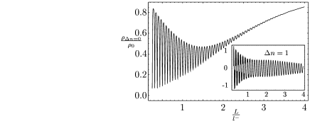
FIG. 6.: The field independent ($\Delta n=0$) part of the DOS for $l^{+}=l^{-}$ (l.h.s) and for $l^{+}=\infty$ (r.h.s); and $pl^{-}=50$. The insets show the $\Delta n=1$ contributions. Higher oscillations ($\Delta n>1$) are similar, but with increased damping.

It is necessary to notice that the oscillative behavior of a persistent current will differ from that obtained for the DoS. In contrary to the dynamical approach to the study of conductance, as a result of which the latter is connected with a current–current correlator, the average thermodynamic current $\langle I(\phi)\rangle$ is defined by the average value of the thermodynamic potential $F$ according to $\langle I(\phi)\rangle=-c\frac{\partial\langle F\rangle}{\partial\phi}$ where the bracket denotes an averaging over the impurity realizations.

At zero temperature the last expression turns to $\langle I(\phi)\rangle=-c\frac{\partial\langle E\rangle}{\partial\phi}$ with $E=\int_{0}^{\mu(\phi)}d\epsilon\,\epsilon\rho(\epsilon,\phi)$ being the total energy of the particles. Expressing DoS $\rho(\epsilon,\phi)$ and the flux dependent Fermi energy $\mu(\phi)$ as $\rho=\langle\rho\rangle+\delta\rho$ and $\mu=\langle\mu\rangle+\delta\mu$ where $\langle\delta\rho\rangle=\langle\delta\mu\rangle=0$ and using in addition the particle number conservation $N={\rm const}=\int_{0}^{\mu(\phi)}d\epsilon\,\rho(\epsilon,\phi)$ to determine $\delta\mu$, $\langle E\rangle$ can be written in the following form:

$$\begin{split}\langle E\rangle=&\int_{0}^{\mu_{0}}d\epsilon\,\epsilon\langle\rho(\epsilon,\phi)\rangle-\frac{\mu_{0}}{\langle\rho\rangle}\int_{0}^{\mu_{0}}d\epsilon\,\langle\delta\rho(\epsilon,\phi)\delta\rho(\mu_{0},\phi)\rangle\\ &+\frac{1}{2\langle\rho\rangle}\Bigl{[}1+\frac{\mu_{0}}{\langle\rho\rangle}\frac{\partial\langle\rho(\mu_{0},\phi)\rangle}{\partial\mu_{0}}\Bigr{]}\int_{0}^{\mu_{0}}d\epsilon_{1}\int_{0}^{\mu_{0}}d\epsilon_{2}\,\langle\delta\rho(\epsilon_{1},\phi)\delta\rho(\epsilon_{2},\phi)\rangle\end{split}$$ (19)

As it is seen from this expression, contributions to the persistent current are given not only by the average value of the DoS but also by the correlator $\langle\delta\rho\delta\rho\rangle$. By expressing the DoS as a difference of the retarded ($G^{+}$) and advanced ($G^{-}$) Green’s functions, the latter correlator is shown to be dominated by $\langle G^{+}G^{-}\rangle$. Characterizing the retarded (advanced) Green’s function by the number of line pairs $m$ ($\overline{m}$) and by the total number of throughgoing lines $n=n^{+}+n^{-}$ ($\overline{n}=\overline{n}^{+}+\overline{n}^{-}$), the oscillating factors in the kernel for the correlator $\langle G^{+}G^{-}\rangle$ will have the form (compare with Eq.(8)) $\cos(p(\epsilon)L(n-\overline{n}))\cos(2\pi\frac{\phi}{\phi_{0}}(n^{+}-n^{-}+\overline{n}^{+}-\overline{n}^{-}))$. The main contribution to the correlator comes from the terms with $n=\overline{n}$, which oscillate with the halved period, [30].

The explanation presented above for the $\frac{\phi_{0}}{2}$ – periodicity of $\langle I(\phi)\rangle$ is connected with the transition from the grand canonical ensemble averaging to the canonical one [9, 12, 13, 18, 19, 31]. Another consideration also seems to be pertinent. For a mesoscopic system the total energy $E$ at $T=0$ is a random parameter. For a fixed chemical potential in the system the number of levels fluctuates from sample to sample. An external magnetic field will periodically change these fluctuations. The correct approach to the problem is to find the distribution function of $E$, which seems to be the same as the one for the DoS, and to calculate the typical value of $E$ by means of averaging. Such averaging will include not only $\langle\rho\rangle$ but also higher moment correlators.

The method presented in this paper makes it possible to calculate all these moments of the DoS [30], as it was done in [23] for a strictly 1d system. Further, the extention to correlators of the local DOS with different energies and different positions allows to study level repulsion.

In conclusion, we have presented a new diagrammatic method which gives an exact result for a one–channel weakly disordered ring threaded by a magnetic flux $\phi$. As an application of the method the DoS of an Aharonov–Bohm ring in the absence of electron–electron interaction is calculated. The result obtained gives an exact dependence of the DoS on the parameters $\phi$, $\epsilon$, $L$ and $l^{\pm}$.

We are thankful for useful discussions with V. N. Prigodin in the early stage of this work. This work was supported by the SFB410.

REFERENCES

- [1] Permanent address: Aserbaijan Academy of Sciences, Institute of Physics, H.Cavid Street 33, Baku
- [2] B. L. Al’tshuler, A. G. Aronov, and B. Z. Spivak, Pis’ma Zh. Eksp. Teor. Fiz. 33, 101 (1981), [JETP Lett. 33, 94 (1981)].
- [3] D. Y. Sharvin and Y. V. Sharvin, Pis’ma Zh. Eksp. Teor. Fiz. 34, 285 (1981), [JETP Lett. 34, 272 (1981)].
- [4] M. Büttiker, Y. Imry, and R. Landauer, Phys. Lett. 96A, 365 (1983).
- [5] R. Landauer and M. Büttiker, Phys. Rev. Lett. 54, 2049 (1985).
- [6] V. Chandrasekhar et al., Phys. Rev. Lett. 67, 3578 (1991).
- [7] D. Mailly, C. Chapelier, and A. Benoit, Phys. Rev. Lett. 70, 2020 (1993).
- [8] L. P. Levy, G. Dolan, J. Dunsmuir, and H. Bouchiat, Phys. Rev. Lett. 64, 2074 (1990).
- [9] H.-F. Cheung, Y. Gefen, E. K. Riedel, and W.-H. Shih, Phys. Rev. B 37, 6050 (1988).
- [10] H.-F. Cheung, E. K. Riedel, and Y. Gefen, Phys. Rev. Lett. 62, 587 (1989).
- [11] Y. Imry, Introduction to mesoscopic physics (Oxford University Press, New York, 1997).
- [12] G. Montambaux, H. Bouchiat, D. Sigeti, and R. Friesner, Phys. Rev. B 42, 7647 (1990).
- [13] H. Bouchiat and G. Montambaux, Phys. Rev. B 44, 1682 (1991).
- [14] K. B. Efetov, Phys. Rev. Lett. 66, 2794 (1991).
- [15] P. Kopietz and K. B. Efetov, Phys. Rev. B 46, 1429 (1992).
- [16] T. Guhr, A. Müller-Groeling, and H. A. Weidenmüller, Physics Reports 299, 189 (1998).
- [17] V. Ambegaokar and U. Eckern, Phys. Rev. Lett. 65, 381 (1990).
- [18] A. Schmid, Phys. Rev. Lett. 66, 80 (1991).
- [19] F. von Oppen and E. K. Riedel, Phys. Rev. Lett. 66, 84 (1991).
- [20] P. Kopietz, Phys. Rev. Lett. 70, 3123 (1993).
- [21] B. L. Al’tshuler, P. A. Lee, and R. A. Webb, Mesoscopic Phenomena in Solids (North–Holland, Amsterdam, 1991).
- [22] V. N. Prigodin, N. F. Hashimzade, and E. P. Nakhmedov, Z. Phys. B 81, 209 (1990).
- [23] B. L. Altshuler and V. N. Prigodin, Zh. Eksp. Teor. Fiz. 95, 348 (1989), [Sov. Phys. JETP 68, 1989].
- [24] N. F. Mott and W. D. Twose, Adv. Phys. 10, 107 (1961).
- [25] V. L. Berezinskii, Zh. Eksp. Teor. Fiz. 65, 1251 (1973), [Sov. Phys. JETP 38, 620, 1974].
- [26] B. I. Halperin, Phys. Rev. B 139, A104 (1965).
- [27] A. A. Gogolin, Zh. Eksp. Teor. Fiz. 83, 2260 (1982), [Sov. Phys. JETP 56, 1309 (1982)].
- [28] A. A. Gogolin, Phys. Rep. 86, 1 (1982).
- [29] B. L. Al’tshuler and B. I. Shklovskii, Sov. Phys. JETP 91, 220 (1986), [Sov. Phys. JETP 64, 127 (1986)].
- [30] H. Feldmann, E. P. Nakhmedov, and R. Oppermann, To be published , in this work, we calculate all higher moments of the DoS to study the total distribution function.
- [31] B. L. Altshuler, Y. Gefen, and Y. Imry, Phys. Rev. Lett. 66, 88 (1991).