Analytic static structure factors and pair–correlation functions
for the unpolarized homogeneous electron gas

Abstract

We propose a simple and accurate model for the electron static structure factors (and corresponding pair–correlation functions) of the 3D unpolarized homogeneous electron gas. Our spin–resolved pair–correlation function is built up with a combination of analytic constraints and fitting procedures to quantum Monte Carlo data, and, in comparison to previous attempts (i) fulfills more known integral and differential properties of the exact pair–correlation function, (ii) is analytic both in real and in reciprocal space, and (iii) accurately interpolates the newest, extensive diffusion–Monte Carlo data of Ortiz, Harris and Ballone [Phys. Rev. Lett. 82, 5317 (1999)]. This can be of interest for the study of electron correlations of real materials and for the construction of new exchange and correlation energy density functionals.

I Introduction

The homogeneous electron gas, a model solid whose positive ionic charges are smeared throughout the whole crystal volume to yield a shapeless, uniform positive background (whence the nickname of jellium) has provided, since the very start of quantum mechanics, a key conceptual reference and a mine of information for solid–state and many–body theorists.[1, 2, 3] Initially it was mostly regarded as an approximation of the true distribution of valence electrons in simple metals, since, in spite of its crudity, it could already account for some of their experimental properties.[4] Although the importance of valence–charge inhomogeneites in real materials was soon recognized (and described first by perturbation[5] and later by self–consistent pseudopotential theory[6]), the homogeneous electron gas stood by itself, over the decades, as an independent active field of theoretical[7] and numerical[8, 9, 10, 11, 12, 13] investigation. One reason for this continued interest is that the model, by ignoring the ionic lattice which makes real materials different from one another, allows the theorists to concentrate on key aspects of the electron–electron interaction. Another reason for caring about such an unrealistic system resides in its connection to the inhomogeneous electron gas:[1, 2, 14] not only does the jellium model represent an obvious limit, but also, through the Density Functional Theory [15] and its Local Density Approximation, it links to a popular and very successful description of real materials.[16] For the latter reason, from the simplest Hartree–Fock approximation [15] to the pioneering QMC simulations,[8] almost any theory of jellium, its electron correlations and its pair–correlation functions has also implied an improved understanding and construction of Kohn–Sham energy functionals.[17, 18]

In this context our work aims at a new simple analytic expression for the pair–correlation function of the homogeneous electron gas, which describes the spatial correlations of electron pairs with prescribed spin orientations. A good model pair–correlation function and static structure factor has its own interest; its availability over a wide density range is crucial for new developments and applications of the Density Functional Theory, through the construction of ab initio exchange and correlation energy functionals in generalized gradient approximations[19] and in other beyond–LDA schemes.[17, 20, 21, 22] As a consequence, over the last 20 years, several authors already proposed ingenious expressions for this or related functions.[21, 23, 24, 25, 26, 27, 28, 29, 30, 31] A first motivation for resuming and improving over previous efforts is the avalaibility, from recent quantum Monte Carlo (QMC) simulations,[10, 13] of a wealth of new numerical results for the pair–correlation functions and static structure factors of jellium. A second motivation comes from the observation that most of the previous models were not spin–resolved and all of them neither fulfilled all the known exact properties, nor were given in analytic, closed form both in real and reciprocal space. Our goal is thus to give a new, spin–resolved expression for the pair–correlation function which is analytic both in real and reciprocal space, automatically incorporates more exact properties than any previous expression, and contains enough free parameters to fit the new QMC results.[13]

We recall the exact properties of the pair–correlation function for the unpolarized jellium in Sec. II. The three subsequent sections are devoted to a description of our general strategy (Sec. III) and of the resulting functional form for the antiparallel– (Sec. IV) and parallel–spin (Sec. V) pair–correlation functions. In Sec. VI we describe our fitting procedure to QMC data.[13] Once the exact constraints are imposed, 18 free parameters (9 for antiparallel spins and 9 for parallel spins) are enough to yield extremely accurate two–dimensional fits of the $\approx 9000+9000$ new QMC data points[13] as a function of the interelectronic distance $r$ and the density parameter $r_{s}$ in the relevant density range $r_{s}\leq 10$. Our results are discussed and compared with the widely used Perdew–Wang[29] model in Sec. VII.

In Sec. VIII we report the correlation energy which corresponds to our model pair–correlation function, and we find that its agreement with the QMC energies,[13] not targeted by our fitting procedure, is as good ($\sim 5$%) as the most popular interpolation formulae for the correlation energy. The last Sec. IX is devoted to conclusions and perspectives.

II Exact properties

We briefly recall many known properties of the pair correlation function of the unpolarized homogeneous electron gas. Its integral properties (sum rules) will be rewritten in terms of $q\to 0$ properties of Fourier transforms, since this choice turns out to be convenient for our subsequent steps. Hartree atomic units are used throughout this work.

A Definitions

For an electronic system the pair–correlation function $g_{\sigma_{1}\sigma_{2}}({\bf r}_{1},{\bf r}_{2})$, if $n_{\sigma}({\bf r})$ is the density of electrons with spin $\sigma=\uparrow$ or $\downarrow$, is defined by

$$n_{\sigma_{1}}({\bf r}_{1})n_{\sigma_{2}}({\bf r}_{2}) g_{\sigma_{1}\sigma_{2}}({\bf r}_{1},{\bf r}_{2})=$$ (2)

$$\langle\Phi|\psi_{\sigma_{1}}^{\dagger}({\bf r}_{1})\psi_{\sigma_{2}}^{\dagger}({\bf r}_{2})\psi_{\sigma_{2}}({\bf r}_{2})\psi_{\sigma_{1}}({\bf r}_{1})|\Phi\rangle$$

and is thus related to the probability of finding two electrons of prescribed spin orientations at positions ${\bf r}_{1}$ and ${\bf r}_{2}$. The normalization of $g$ is such that the expected number of electrons of spin $\sigma_{2}$ in the volume $dV$ at ${\bf r}_{2}$ when another electron of spin $\sigma_{1}$ is known to be at ${\bf r}_{1}$ is given by

$$dN({\bf r}_{2}\sigma_{2}|{\bf r}_{1}\sigma_{1})=n_{\sigma_{2}}({\bf r}_{2})\,g_{\sigma_{1}\sigma_{2}}({\bf r}_{1},{\bf r}_{2})\,dV;$$ (3)

the lack of any correlation amounts, then, to the condition $g_{\sigma_{1}\sigma_{2}}({\bf r}_{1},{\bf r}_{2})=1$. In the spin–unpolarized jellium the electronic spin density $n_{\uparrow}({\bf r})=n_{\downarrow}({\bf r})=n/2=(8\pi r_{s}^{3}/3)^{-1}$ is uniform in space (i.e. independent of ${\bf r}$), [32] so $g_{\sigma_{1}\sigma_{2}}({\bf r}_{1},{\bf r}_{2})$ only depends on the distance between the two electrons $r=|{\bf r}_{1}-{\bf r}_{2}|$. The static structure factor $S(q)$ is directly related to the Fourier transform of the pair–correlation function. For an unpolarized homogeneous electron gas, after introducing the Fermi wavevector $q_{F}=(3\pi^{2}\,n)^{1/3}=\alpha/r_{s}$, with $\alpha=(9\pi/4)^{1/3}$, the scaled variables $\rho=q_{F}\,r$ and $k=q/q_{F}$ are often convenient. With these variables the static structure factors are written as

$$S_{\uparrow\downarrow}(k) = \frac{2}{3\,\pi}\int_{0}^{\infty}d\rho\,\left[g_{\uparrow\downarrow}(\rho)-1\right]\,\rho^{2}\frac{\sin(k\,\rho)}{k\,\rho}$$ (4)

$$S_{\uparrow\uparrow}(k) = 1+\frac{2}{3\,\pi}\int_{0}^{\infty}d\rho\,\left[g_{\uparrow\uparrow}(\rho)-1\right]\,\rho^{2}\frac{\sin(k\,\rho)}{k\,\rho}$$ (5)

and the total pair–correlation function and static structure factor are given by:

$$g(\rho;r_{s}) = \frac{1}{2}\left[g_{\uparrow\uparrow}(\rho;r_{s})+g_{\uparrow\downarrow}(\rho;r_{s})\right]$$ (6)

$$S(k;r_{s}) = S_{\uparrow\uparrow}(k;r_{s})+S_{\uparrow\downarrow}(k;r_{s}).$$ (7)

B Pair–correlation function near $r=0$

The behavior of $g_{\sigma_{1}\sigma_{2}}(r;r_{s})$ in the $r\to 0$ limit can be directly obtained from the many–body Schrödinger equation when two electrons approach each other (cusp conditions):[23, 33, 34]

$$\frac{\partial}{\partial r}g_{\uparrow\downarrow}(r;r_{s})\biggr{|}_{r\to 0} = g_{\uparrow\downarrow}(r\to 0;r_{s})\neq 0$$ (8)

$$\frac{\partial}{\partial r}g_{\uparrow\uparrow}(r;r_{s})\biggr{|}_{r\to 0} = g_{\uparrow\uparrow}(r\to 0;r_{s})=0$$ (9)

$$\frac{\partial^{3}}{\partial r^{3}}g_{\uparrow\uparrow}(r;r_{s})\biggr{|}_{r\to 0} = \frac{3}{2}\frac{\partial^{2}}{\partial r^{2}}g_{\uparrow\uparrow}(r;r_{s})\biggr{|}_{r\to 0}\neq 0.$$ (10)

Eqs. (8)–(10) hold for any 3D–system of $N$ fermions interacting via the two–body repulsive Coulomb potential.

C Structure factor near $q=0$

The conservation of particles in the system implies the relations:

$$S_{\uparrow\downarrow}(q\to 0;r_{s})=S_{\uparrow\uparrow}(q\to 0;r_{s})=0.$$ (11)

The asymmetry between the definitions (4) and (5) leads to the two well–known sum rules for $g_{\uparrow\downarrow}$ and $g_{\uparrow\uparrow}$ (see for instance Ref. [23]).

The long–wavelength behavior of the total static structure factor of Eq. (7) is determined by the plasmon contribution, proportional to $q^{2}$, and by the single–pair and multipair quasiparticle–quasihole excitation contributions, proportional to $q^{5}$ and $q^{4}$ respectively:[3, 35]

$$S(q\to 0;r_{s})=\frac{q^{2}}{2\,\omega_{p}(r_{s})}+C\,q^{4}+{\cal O}(q^{5}),$$ (12)

where $\omega_{p}(r_{s})=\sqrt{3/r_{s}^{3}}$ is the classical plasma frequency. In the paramagnetic gas, the parallel and antiparallel–spin contribution to the plasma mode is the same. Moreover, to build up model functions for the spin–resolved $S_{\sigma_{1}\sigma_{2}}$, it’s crucial to include the following property of the so–called magnetic structure factor $S_{\uparrow\uparrow}-S_{\uparrow\downarrow}$:

$$S_{\uparrow\uparrow}-S_{\uparrow\downarrow}\big{|}_{k\to 0}=\frac{3}{4}k-\frac{k^{3}}{16}+{\cal O}(k^{4}),$$ (13)

where the scaled variable $k=q/q_{F}$ has been used. Eq. (13) is valid in the framework of the random–phase approximation[3] (RPA) and can be obtained from a series expansion of $S_{\uparrow\downarrow}^{\rm RPA}(k)$ near $k=0$ (Ref. [36]), and from the corresponding expansion of the total $S^{\rm RPA}$ (see for instance Ref. [37]). Since in the $k\to 0$ limit RPA is exact,[3, 37, 38, 39] we expect Eq. (13) to hold for the exact structure factor as well. From Eqs. (12) and (13) we can write the small–$k$ expansion of $S_{\sigma_{1}\sigma_{2}}$:

$$S_{\uparrow\downarrow}\big{|}_{k\to 0} = -\frac{3}{8}k+\frac{q_{F}^{2}\,k^{2}}{4\,\omega_{p}(r_{s})}+\frac{k^{3}}{32}+{\cal O}(k^{4})$$ (14)

$$S_{\uparrow\uparrow}\big{|}_{k\to 0} = \frac{3}{8}k+\frac{q_{F}^{2}\,k^{2}}{4\,\omega_{p}(r_{s})}-\frac{k^{3}}{32}+{\cal O}(k^{4}).$$ (15)

D Correlation energy

The electron–electron potential energy is, as known, given by the sum of repulsive two–body Coulomb terms:

$$U=\frac{1}{2}\sum_{i\neq j}^{N}\frac{1}{|{\bf r}_{i}-{\bf r}_{j}|}.$$ (16)

Its ground–state expectation value (per electron), in a homogenous electron gas of density $r_{s}$, is given by the following integral over the pair–correlation function:

$$\langle U\rangle_{r_{s}}=\frac{3}{2\,\alpha^{2}\,r_{s}}\int_{0}^{\infty}\left[g(\rho;r_{s})-1\right]\,\rho\,d\rho.$$ (17)

By the virial theorem [40] and the usual definition of the correlation energy $\epsilon_{c}$ as total electronic energy minus Hartree–Fock energy, we have:

$$\langle U\rangle_{r_{s}}=-\frac{3\,q_{F}}{4\,\pi}+\frac{1}{r_{s}}\frac{d}{dr_{s}}\left[r_{s}^{2}\,\epsilon_{c}(r_{s})\right]$$ (18)

Putting together Eqs. (17) and (18) one obtains the known relation between $g(\rho;\,r_{s})$ and the exchange and correlation energy:

$$\epsilon_{xc}=-\frac{3q_{F}}{4\pi}+\epsilon_{c}=\frac{3}{2\alpha^{2}r_{s}^{2}}\int_{0}^{\infty}d\rho\,\rho\int_{0}^{r_{s}}dr_{s}^{\prime}\left[g(\rho;\,r_{s}^{\prime})-1\right]$$ (19)

The same relation can be obtained in a more general way [17] by the Hellmann–Feynman theorem and the coupling–constant average of $g(\rho;\,r_{s})$, which, for the homogeneous system is just the average over $r_{s}$:

$$\overline{g}(\rho;\,r_{s})=\frac{1}{r_{s}}\int_{0}^{r_{s}}g(\rho;\,r_{s}^{\prime})\,dr_{s}^{\prime}.$$ (20)

The function $\overline{g}(\rho;\,r_{s})$ is directly related to the exchange and correlation hole[17, 29] of the electron gas.

We have recalled these relations because we will later check our analytical expressions for $g(\rho;\,r_{s})$ against available energy data, and also because, among other constraints, we want our functional form of $g(\rho;r_{s})$ to be consistent with the high–density limit of $\epsilon_{c}(r_{s})$:

$$\epsilon_{c}(r_{s}\to 0)=A\,\ln r_{s}+B+C\,r_{s}\,\ln r_{s}+D\,r_{s}$$ (21)

where $A$, $B$, $C$ and $D$ are known constants,[38, 41, 42, 43, 44, 45, 46] $A=(1-\ln 2)/\pi^{2}$, $B=-0.0469205$, $C=0.0092292$, $D=-0.01$, and the next leading term is ${\cal O}(r_{s}^{2}\ln r_{s})$.

III General strategy

We study the antiparallel and parallel–spin correlation functions both in real and reciprocal space and we split them, as usually, into exchange and correlation according to:

$$g_{\uparrow\downarrow}(\rho;r_{s}) = 1+g^{c}_{\uparrow\downarrow}(\rho;r_{s})$$ (22)

$$g_{\uparrow\uparrow}(\rho;r_{s}) = g_{ex}(\rho)+g^{c}_{\uparrow\uparrow}(\rho;r_{s})$$ (23)

$$S_{\uparrow\downarrow}(k;r_{s}) = S^{c}_{\uparrow\downarrow}(k;r_{s})$$ (24)

$$S_{\uparrow\uparrow}(k;r_{s}) = S_{ex}(k)+S^{c}_{\uparrow\uparrow}(k;r_{s})$$ (25)

where the exchange functions, given by the Hartree–Fock approximation, are equal to:

$$g_{ex}(\rho) = 1-9\left(\frac{\sin\rho-\rho\cos\rho}{\rho^{3}}\right)^{2}$$ (26)

$$S_{ex}(k) = \cases{3k/4-k^{3}/16&for $k\leq 2$\cr 1&for $k>2$\cr}$$ (27)

and our model only concerns the correlation part. Putting together Eqs. (7), (12), (24), (25) and (27) one finds a well–known result: in the total $S=S_{ex}+S^{c}_{\uparrow\downarrow}+S^{c}_{\uparrow\uparrow}$, the linear term of $S_{ex}(k)$, $3k/4$, which dominates its small–$k$ behavior (and corresponds to a large–$\rho$ leading term $\propto 1/\rho^{4}$ of $g_{ex}$) exactly cancels the small–$k$ leading term of the correlation part $S^{c}_{\uparrow\downarrow}+S^{c}_{\uparrow\uparrow}$. This property has been incorporated in several previous functional forms for the total $g$, as the widely used Perdew–Wang[29] model (hereafter PW) where, however, the $k^{2}$ coefficient in the small–$k$ expansion of $S(k)$ is slightly different from the exact one [Eq. (12)], because of spurious $k^{2}$ contributions from their $\langle g_{x}\rangle$ [Eq. (19) of Ref.[29]] and from their short–range part of $g_{c}$ [Eq. (37) of Ref.[29]].

The $k\to 0$ limit of Eq. (13) seems, instead, to be less known: even the best–to–date spin–resolved PW[29] model does not incorporate such a non–trivial analytic property, which can alternatively be expressed as $S^{c}_{\uparrow\uparrow}$ beeing identical to $S^{c}_{\uparrow\downarrow}$ in the the small–$k$ limit and corresponds to a visible feature of the magnetic structure factor (see Sec. VII). Our goal is to produce simple and practical analytical functional forms for $S^{c}_{\uparrow\downarrow}(k;r_{s})$ and $S^{c}_{\uparrow\uparrow}(k;r_{s})$ [and hence $g^{c}_{\uparrow\downarrow}(\rho,r_{s})$ and $g^{c}_{\uparrow\uparrow}(\rho,r_{s})$] which satisfy all the physical properties of Sec. II and have enough variational flexibility to accurately interpolate the QMC data of Ortiz, Harris and Ballone.[13]

To do this, let’s start with a few simple considerations about spherical Fourier transforms: $S^{c}_{\sigma_{1}\sigma_{2}}(k)$ and $g^{c}_{\sigma_{1}\sigma_{2}}(\rho)$ are related to one another by an integration like Eq. (4). The function $\sin(k\rho)/k\rho$ is an even function, i. e. its odd derivatives in $k=0$ (or $\rho=0$) are all equal to zero. However, the small–$\rho$ and the small–$k$ properties of $g$ and $S$ tell us that they must have non–zero odd derivatives in $\rho=0$ and $k=0$. This is achieved if (and only if), as the integration variable goes to infinity, the integrand goes to zero slowly enough as to avoid absolute convergence, so that differentiation within the integral sign is not allowed. It is easy to establish a connection between the large–$k$ (large–$\rho$) behavior of $S$ ($g$) and the odd derivatives in $\rho=0$ ($k=0$) of $g$ ($S$): a derivative of $g$ in $\rho=0$ of order $2n+1$ corresponds, in $S$, to a large–$k$ term $\propto 1/k^{2n+4}$ and viceversa. This simple relation was used in Ref.[23] to obtain the large–$k$ expansion of $S_{\sigma_{1}\sigma_{2}}$ from the cusp conditions of Eqs. (8) and (10). These elementary considerations lead us to write down a very simple functional form $S^{c}$ in reciprocal space which automatically has the exact small–$k$ and large–$k$ behavior. Its spherical Fourier transform $g^{c}$ is analytic and closed–form, consisting of the same kind of functions used in reciprocal space. We thus have an equally simple expression for $S^{c}$ and $g^{c}$.

We begin by studying the antiparallel–spin part, and do it in several steps. First (IV A) we choose our functional form. Then (IV B) we impose to it the properties of Sec. II. At this point we are left with 6 free parameters, which, independently for each available $r_{s}$, are used to accurately fit the QMC data both in real and reciprocal space, as done in Ref. [10]. In our case, however, the $r_{s}$ dependence of each of the 6 optimal parameters turns out to be both regular and monotonic. We then try to represent each of them as a simple function of $r_{s}$ in such a way that (i) as $r_{s}\to 0$ the exact high–density expansion of the correlation energy [Eq. (21)] is recovered (IV C), and (ii) for finite $r_{s}\leq 10$ an optimal global fit of all the QMC data[13] is obtained (VI). We apply the same strategy to the parallel–spin part (V). Besides the excellent quality of the final fits of $g$ and $S$, we see that even the resulting correlation energy, not targeted by our fitting strategy except at $r_{s}\to 0$, turns out to be in good agreement (within $5\%$) with the corresponding QMC results[13] at any $r_{s}$. We compare our correlation energy with the most popular interpolation formulae and we discuss their relative efficiency in fitting the new QMC energies.[13]

IV Antiparallel spins

A Functional form

In reciprocal space our functional form is simply written as:

$$S^{c}_{\uparrow\downarrow}(k;r_{s}) = \exp\left[-b^{\uparrow\downarrow}(r_{s})\,k\right]\,\sum_{n=1}^{6}c_{n}^{\uparrow\downarrow}(r_{s})\,k^{n}+$$ (29)

$$\frac{\alpha_{6}^{\uparrow\downarrow}(r_{s})\,k^{8}+\alpha_{4}^{\uparrow\downarrow}(r_{s})\,k^{10}}{\left[(a^{\uparrow\downarrow})^{2}+k^{2}\right]^{7}};$$

as mentioned, the corresponding $g^{c}_{\uparrow\downarrow}$ amounts to a linear combination of the same kind of functions[47] in real space [see App. A, Eq. (A3)]. Two types of functions appear in Eq. (29): the first one, an exponential cut–off times a truncated power series, fully characterizes the long–wavelength behavior of $S$, while the second one entirely determines its large–$k$ expansion. The leading term as $k\to\infty$ is of order $k^{-4}$, as exactly known from the cusp condition;[23, 33] in real space the short–range behavior is thus entirely determined by the parameter $\alpha_{4}^{\uparrow\downarrow}(r_{s})$:

$$\frac{\partial}{\partial\rho}g_{\uparrow\downarrow}(\rho;r_{s})\biggr{|}_{\rho\to 0} = -\frac{3\pi}{4}\alpha_{4}^{\uparrow\downarrow}(r_{s})$$ (30)

$$g_{\uparrow\downarrow}(\rho=0;r_{s}) = -\frac{3\pi}{4}q_{F}(r_{s})\alpha_{4}^{\uparrow\downarrow}(r_{s}).$$ (31)

B Physical constraints

The $k\to 0$ conditions of Subsec. II C are easily imposed:

$$c_{1}^{\uparrow\downarrow} = -\frac{3}{8}$$ (32)

$$c_{2}^{\uparrow\downarrow} = b^{\uparrow\downarrow}c_{1}^{\uparrow\downarrow}+\frac{q_{F}^{2}}{4\omega_{p}}$$ (33)

$$c_{3}^{\uparrow\downarrow} = (b^{\uparrow\downarrow})^{2}\frac{c_{1}^{\uparrow\downarrow}}{2}+b^{\uparrow\downarrow}\frac{q_{F}^{2}}{4\omega_{p}}+\frac{1}{32}.$$ (34)

The cusp condition of Eq. (8) fixes a simple relation between $\alpha_{6}^{\uparrow\downarrow}$ and the other parameters:

$$\alpha_{6}^{\uparrow\downarrow} = (a^{\uparrow\downarrow})^{3}\Biggl{\{}\alpha_{4}^{\uparrow\downarrow}\left(\frac{11}{a^{\uparrow\downarrow}}-\frac{512}{21}q_{F}\right)-$$ (36)

$$\frac{2048}{21\pi}\left[\frac{1}{3}+\sum_{n=1}^{6}c_{n}^{\uparrow\downarrow}\frac{(n+2)!}{(b^{\uparrow\downarrow})^{n+3}}\right]\Biggr{\}}$$

After imposing all the $\uparrow\downarrow$ physical conditions, our model [Eq. (29)] is left with 6 free parameters: the two exponential cut–offs ($a^{\uparrow\downarrow}$ in real space and $b^{\uparrow\downarrow}$ in reciprocal space), the parameter $\alpha_{4}^{\uparrow\downarrow}$, which determines the short–range behavior of $g(r)$, and the 3 linear parameters $c_{4}^{\uparrow\downarrow}$, $c_{5}^{\uparrow\downarrow}$ and $c_{6}^{\uparrow\downarrow}$, which will be used to further increase the variational flexibility and fit the numerical $g_{\uparrow\downarrow}$ obtained from QMC simulations.[13] The dependence of these free parameters on $r_{s}$ will be determined according to the strategy summarized in Sec. III and detailed in the following Subsec. IV C and Sec. V.

C High–density expansion

As anticipated in Subsec. II D, we want our pair–correlation function such that its $\uparrow\downarrow$ and $\uparrow\uparrow$ contributions automatically fulfill the high–density limit of the correlation energy. We thus fix the $r_{s}\to 0$ limit of our free parameters by means of Eqs. (17), (18) and (21). Our antiparallel contribution to the expectation value of the potential energy $U=U_{\uparrow\downarrow}+U_{\uparrow\uparrow}$ is simply given by:

$$U_{\uparrow\downarrow}=\frac{q_{F}}{\pi}\sum_{n=1}^{6}\frac{c_{n}^{\uparrow\downarrow}n!}{(b^{\uparrow\downarrow})^{n+1}}+\frac{q_{F}}{2048}\left[\frac{7\alpha_{6}^{\uparrow\downarrow}}{(a^{\uparrow\downarrow})^{5}}+\frac{21\alpha_{4}^{\uparrow\downarrow}}{(a^{\uparrow\downarrow})^{3}}\right].$$ (37)

In the high–density limit, the correlation–energy constraint of Eq. (21) translates into the following condition on $\langle U_{\uparrow\downarrow}\rangle_{r_{s}}$:

$$\langle U_{\uparrow\downarrow}\rangle_{r_{s}\to 0}=2\,A_{\uparrow\downarrow}\,\ln r_{s}+\left(A_{\uparrow\downarrow}+2\,B_{\uparrow\downarrow}\right)+{\cal O}(r_{s}\,\ln r_{s})$$ (38)

where, comparing to Eq. (21), $A_{\uparrow\downarrow}$ is simply given[43] by $\frac{1}{2}A$. To determine $B_{\uparrow\downarrow}$ we recall that the constant $B$ in Eq. (21) is the sum of two contributions: a second–order exchange term, $B^{(2)}_{exc}$, which only concerns the $\uparrow\uparrow$ part, and a direct term, $B_{d}$, which is, instead, equally split (in the unpolarized gas) between $\uparrow\uparrow$ and $\uparrow\downarrow$. Hence, $B_{\uparrow\downarrow}=B_{d}/2$. Both $B^{(2)}_{exc}$ and $B_{d}$ have been evaluated exactly.[44, 45]

Provided that the 3 linear parameters $c_{4}^{\uparrow\downarrow}$, $c_{5}^{\uparrow\downarrow}$ and $c_{6}^{\uparrow\downarrow}$ remain finite as $r_{s}\to 0$, the exact high–density limit of Eq. (38) amounts to the following conditions:

$$\alpha_{4}^{\uparrow\downarrow}(r_{s}\to 0) = \frac{1+k_{1}r_{s}\ln r_{s}+k_{2}r_{s}+{\cal O}(r_{s}^{2}\ln r_{s})}{-3\pi q_{F}/4}$$ (39)

$$b^{\uparrow\downarrow}(r_{s}\to 0) = \left(\frac{4}{9\pi}\right)^{1/3}\pi\sqrt{\frac{3}{r_{s}}}+{\cal O}(r_{s}^{0})$$ (40)

$$a^{\uparrow\downarrow}(r_{s}\to 0) = {\rm const.}+{\cal O}(r_{s})\equiv a^{\uparrow\downarrow}+{\cal O}(r_{s})$$ (41)

where $k_{1}$ and $k_{2}$ depend on $A_{\uparrow\downarrow}$, $B_{\uparrow\downarrow}$ and $a^{\uparrow\downarrow}$:

$$k_{1} = \frac{18\pi(a^{\uparrow\downarrow})^{2}}{\alpha}A_{\uparrow\downarrow}$$ (42)

$$k_{2} = \frac{729}{64}\frac{(a^{\uparrow\downarrow})^{2}}{\alpha^{4}}-\frac{21}{64}\frac{1}{a^{\uparrow\downarrow}\alpha}+$$ (44)

$$\frac{9(a^{\uparrow\downarrow})^{2}\pi}{2\alpha}(A_{\uparrow\downarrow}+2B_{\uparrow\downarrow}).$$

Inserting Eq. (39) into Eq. (31) we see that in our model, once the high–density expansion of $\epsilon_{c}(r_{s})$ is fixed, the $r_{s}\to 0$ limit of $g(\rho=0;r_{s})$ is also fixed to the form $1+Cr_{s}\ln r_{s}+{\cal O}(r_{s})$. The corresponding exact form[48] is, up to orders $r_{s}^{2}$, $1+C_{1}r_{s}+C_{2}r_{s}^{2}\ln r_{s}$, thus slightly different from ours. Evidently, the simple functional form of Eq. (29) does not correctly describe the short–range behavior of the Coulomb hole at very high densities. It is worthwhile to point out that this contradiction is due to the exponential cut–off times a truncated power series in real space [Eq. (A3)], and emerges when the cusp condition of Eq. (8) is imposed to it. The relevance of this limitation, which only concerns densities $r_{s}\lesssim 0.1$, will be discussed in next Sec. VII.

V Parallel spins

A Functional form

For the correlation part of the $\uparrow\uparrow$ pair–distribution function we apply the same strategy used for the antiparallel–spin case. In reciprocal space we thus have:

$$S^{c}_{\uparrow\uparrow}(k;r_{s}) = \exp\left[-b^{\uparrow\uparrow}(r_{s})\,k\right]\,\sum_{n=1}^{6}c_{n}^{\uparrow\uparrow}(r_{s})k^{n}+$$ (46)

$$\frac{\alpha_{10}^{\uparrow\uparrow}(r_{s})k^{8}+\alpha_{8}^{\uparrow\uparrow}(r_{s})k^{10}+\alpha_{6}^{\uparrow\uparrow}(r_{s})k^{12}}{\left[(a^{\uparrow\uparrow})^{2}+k^{2}\right]^{9}}$$

which again corresponds, in real space, to a linear combination of the same kind of functions[47] [see App. A, Eq. (A8)]. The long–wavelength term has the same form as the $\uparrow\downarrow$ part. The large–$k$ term describes the short–range behavior of $g_{\uparrow\uparrow}$: the cusp condition of Eq. (10) tells us that, as $k\to\infty$, the leading term of $S^{c}_{\uparrow\uparrow}$ must be of order $k^{-6}$. With respect to the $\uparrow\downarrow$ case, one more parameter is needed for the large–$k$ term to satisfy the Pauli principle. As in the antiparallel–spin case, the short–range properties of $g_{\uparrow\uparrow}$ are characterized by the $\alpha_{6}^{\uparrow\uparrow}$ parameter:

$$\frac{\partial^{3}}{\partial\rho^{3}}g_{\uparrow\uparrow}(\rho;r_{s})\biggr{|}_{\rho\to 0} = \frac{3\pi}{8}\alpha_{6}^{\uparrow\uparrow}(r_{s})$$ (47)

$$\frac{\partial^{2}}{\partial\rho^{2}}g_{\uparrow\uparrow}(\rho;r_{s})\biggr{|}_{\rho\to 0} = \frac{\pi}{4}q_{F}(r_{s})\alpha_{6}^{\uparrow\uparrow}(r_{s}).$$ (48)

B Physical constraints

The small–$k$ properties imply, for the $\uparrow\uparrow$ case, identical constraints as for the $\uparrow\downarrow$ case [see Eqs. (32), (33) and (34)].

The Pauli principle and the cusp condition of Eqs. (9) and (10) fix the dependence of $\alpha_{8}^{\uparrow\uparrow}$ and $\alpha_{10}^{\uparrow\uparrow}$ on the remaining parameters:

$$\alpha_{8}^{\uparrow\uparrow} = \frac{2048}{3\pi}(a^{\uparrow\uparrow})^{5}\sum_{n=1}^{6}\frac{c_{n}^{\uparrow\uparrow}}{(b^{\uparrow\uparrow})^{n+3}}\left[(n+2)!-\frac{5(n+4)!}{(a^{\uparrow\uparrow}b^{\uparrow\uparrow})^{2}}\right]$$ (50)

$$+\frac{4096}{33\pi}(a^{\uparrow\uparrow})^{3}-\alpha_{6}^{\uparrow\uparrow}(a^{\uparrow\uparrow})^{3}\left(\frac{2560q_{F}}{33}+\frac{26}{a^{\uparrow\uparrow}}\right)$$

$$\alpha_{10}^{\uparrow\uparrow} = \frac{2048}{3\pi}(a^{\uparrow\uparrow})^{7}\sum_{n=1}^{6}\frac{c_{n}^{\uparrow\uparrow}}{(b^{\uparrow\uparrow})^{n+3}}\left[\frac{(n+4)!}{(a^{\uparrow\uparrow}b^{\uparrow\uparrow})^{2}}-\frac{13}{3}(n+2)!\right]$$ (52)

$$-\frac{4096}{15\pi}(a^{\uparrow\uparrow})^{5}+\frac{\alpha_{6}^{\uparrow\uparrow}}{3}(a^{\uparrow\uparrow})^{5}\left(\frac{143}{a^{\uparrow\uparrow}}+512q_{F}\right).$$

The cusp condition of Eq. (10) is not included in the PW model. As in the antiparallel–spin case, we have 6 free parameters: the exponential cut–off in real space, $a^{\uparrow\uparrow}$, the exponential cut–off in reciprocal space, $b^{\uparrow\uparrow}$, the $\alpha_{6}^{\uparrow\uparrow}$ parameter, which determines the short–range behavior of $g_{\uparrow\uparrow}$, and the three linear parameters $c_{4}^{\uparrow\uparrow}$, $c_{5}^{\uparrow\uparrow}$ and $c_{6}^{\uparrow\uparrow}$, which are used to fit the oscillatory behavior of $g_{\uparrow\uparrow}$.

C High–density expansion

The contribution to the expectation value of the potential energy due to the correlation part of our $g_{\uparrow\uparrow}$ ($U_{\uparrow\uparrow}=-3q_{F}/4\pi+U^{c}_{\uparrow\uparrow}$) is:

$$U_{\uparrow\uparrow}^{c} = \frac{q_{F}}{\pi}\sum_{n=1}^{6}\frac{c_{n}^{\uparrow\uparrow}n!}{(b^{\uparrow\uparrow})^{n+1}}+\frac{q_{F}}{65536}\biggl{[}\frac{35\,\alpha_{10}^{\uparrow\uparrow}}{(a^{\uparrow\uparrow})^{9}}+\frac{45\,\alpha_{8}^{\uparrow\uparrow}}{(a^{\uparrow\uparrow})^{7}}+$$ (54)

$$+\frac{99\,\alpha_{6}^{\uparrow\uparrow}}{(a^{\uparrow\uparrow})^{5}}\biggr{]}$$

As $r_{s}\to 0$, the condition on $U_{\uparrow\uparrow}^{c}$ is identical to Eq. (38), where[43] $A_{\uparrow\uparrow}=\frac{1}{2}A$, and $B_{\uparrow\uparrow}=B_{exc}^{(2)}+\frac{1}{2}B_{d}$. As in the $\uparrow\downarrow$ case, the exact $r_{s}\to 0$ expansion of $U_{\uparrow\uparrow}^{c}$ implies for the two exponential cut–offs in real ($a^{\uparrow\uparrow}$) and reciprocal space ($b^{\uparrow\uparrow}$) identical conditions as Eqs. (40) and (41). For $\alpha_{6}^{\uparrow\uparrow}$ the condition is similar to Eq. (39):

$$\alpha_{6}^{\uparrow\uparrow}(r_{s}\to 0) = \frac{4}{\pi q_{F}}\biggl{[}\frac{2}{5}+p_{1}r_{s}\ln r_{s}+p_{2}r_{s}+$$ (56)

$$+{\cal O}(r_{s}^{2}\ln r_{s})\biggr{]},$$

where $p_{1}$ and $p_{2}$ depend on $A_{\uparrow\uparrow}$, $B_{\uparrow\uparrow}$ and $a^{\uparrow\uparrow}$ through equations similar to Eqs. (42) and (44). From Eqs. (48) and (56) one can see that, as expected, when $r_{s}\to 0$, $g_{\uparrow\uparrow}^{\prime\prime}(\rho=0)$ goes to the Hartree–Fock value $2/5$. As in the antiparallel–spin case, the high–density limit of the correlation energy fixes the $r_{s}\to 0$ expansion of $g_{\uparrow\uparrow}^{\prime\prime}(\rho=0;r_{s})$. The exact $g_{\uparrow\uparrow}^{\prime\prime}(\rho=0;r_{s}\to 0)$ should have the form[23] $2/5+{\cal O}(r_{s})$, while our functional form gives $2/5+{\cal O}(r_{s}\ln r_{s})$. Again, we find that in real space the simple exponential cut–off times a truncated power series [Eq. (A8)] does not correctly describe the short range Coulomb interactions at very high densities.

VI Fit to QMC data

For each available density in the range $0.8\leq r_{s}\leq 10$ (i.e. $r_{s}=0.8$, 1, 2, 3, 4, 5, 8 and 10) we performed a best fit of the 6 free parameters to the QMC data,[13] separately for the $\uparrow\downarrow$ and the $\uparrow\uparrow$ parts. The $r_{s}$ dependence of the parameters turns out to be quite smooth and monotonic and well described by the following functional forms ( which also take into account the exact high–density limit of Eqs. (39)–(41) and (56) and guarantee the exact low–density expansion of the resulting correlation energy[8, 18, 41, 49, 50] $d_{1}r_{s}^{-1}+d_{2}r_{s}^{-3/2}$):

$$\alpha_{4}^{\uparrow\downarrow}(r_{s}) = -\frac{4\left[1-k_{1}(a^{\uparrow\downarrow})r_{s}\ln\left(1+\tilde{k_{2}}(a^{\uparrow\downarrow})/r_{s}\right)\right]}{3\pi q_{F}\left(1+k_{3}r_{s}^{2}\right)}$$ (57)

$$\alpha_{6}^{\uparrow\uparrow}(r_{s}) = \frac{8\left[1-p_{1}(a^{\uparrow\uparrow})r_{s}\ln\left(1+p_{2}(a^{\uparrow\uparrow})/r_{s}\right)\right]}{5\pi q_{F}\left(1+p_{3}r_{s}^{2}\right)}$$ (58)

$$a^{\sigma_{1}\sigma_{2}}(r_{s}) = a^{\sigma_{1}\sigma_{2}}$$ (59)

$$b^{\sigma_{1}\sigma_{2}}(r_{s}) = \left(\frac{4}{9\pi}\right)^{1/3}\pi\sqrt{\frac{3}{r_{s}}}+b_{1}^{\sigma_{1}\sigma_{2}}$$ (60)

$$c_{n}^{\sigma_{1}\sigma_{2}}(r_{s}) = \frac{\lambda_{n}^{\sigma_{1}\sigma_{2}}+\gamma_{n}^{\sigma_{1}\sigma_{2}}r_{s}}{1+r_{s}^{3/2}}\;\;\;\;\;\;\;\;n=4,5,6$$ (61)

where $k_{1}(a^{\uparrow\downarrow})$ is given by Eq. (42), and $\tilde{k_{2}}(a^{\uparrow\downarrow})$, $p_{1}(a^{\uparrow\uparrow})$ and $p_{2}(a^{\uparrow\uparrow})$ are equal to:

$$\tilde{k_{2}}(a^{\uparrow\downarrow}) = \exp\biggl{[}\frac{7}{384\pi(a^{\uparrow\downarrow})^{3}A_{\uparrow\downarrow}}-\frac{81}{128\pi\alpha^{3}A_{\uparrow\downarrow}}$$ (63)

$$-\frac{B_{\uparrow\downarrow}}{A_{\uparrow\downarrow}}-\frac{1}{2}\biggr{]}$$

$$p_{1}(a^{\uparrow\uparrow}) = \frac{33\pi A_{\uparrow\uparrow}(a^{\uparrow\uparrow})^{4}}{\alpha}$$ (64)

$$p_{2}(a^{\uparrow\uparrow}) = \exp\biggl{[}\frac{7}{960\pi(a^{\uparrow\uparrow})^{5}A_{\uparrow\uparrow}}-\frac{81}{128\pi\alpha^{3}A_{\uparrow\uparrow}}$$ (66)

$$-\frac{B_{\uparrow\uparrow}}{A_{\uparrow\uparrow}}-\frac{1}{2}\biggr{]}.$$

The 9 constants for $\uparrow\downarrow$ and the 9 constants for $\uparrow\uparrow$ have been fixed by a two–dimensional best fit to the QMC data in real and reciprocal space (9368+9368 data points). The efficiency of our interpolation scheme has been tested by performing preliminary fits in wich some of the available $r_{s}$ were not included and then verifying that the interpolated $g$ and $S$ were in good agreement with the corresponding QMC quantities for the excluded $r_{s}$. Since this was always the case, we included all the available $r_{s}$ in order to have optimal values for our final parameters. We thus expect our $g$ and $S$ to be very reliable and accurate in the whole density range $r_{s}\in[0.8,10]$. The optimal 9 parameters which define our best antiparallel–spin model are: $a^{\uparrow\downarrow}=0.838$, $k_{3}=0.141$, $b_{1}^{\uparrow\downarrow}=3.27$, $\lambda_{4}^{\uparrow\downarrow}=-78$, $\gamma_{4}^{\uparrow\downarrow}=28$, $\lambda_{5}^{\uparrow\downarrow}=216$, $\gamma_{5}^{\uparrow\downarrow}=-124$, $\lambda_{6}^{\uparrow\downarrow}=-140$, $\gamma_{6}^{\uparrow\downarrow}=55$, and the other 9 parameters for the parallel–spin part are: $a^{\uparrow\uparrow}=1.32$, $p_{3}=0.015$, $b_{1}^{\uparrow\uparrow}=3.47$, $\lambda_{4}^{\uparrow\uparrow}=98$, $\gamma_{4}^{\uparrow\uparrow}=-36$, $\lambda_{5}^{\uparrow\uparrow}=-295$, $\gamma_{5}^{\uparrow\uparrow}=74$, $\lambda_{6}^{\uparrow\uparrow}=170$, $\gamma_{6}^{\uparrow\uparrow}=-13$.

VII Results in real and reciprocal space

After fixing the $9+9$ parameters which fully specify our model, we are now ready to present, in Fig. 1, our real–space pair–correlation function $g_{\sigma_{1}\sigma_{2}}$, shown as a solid line, as a function of the scaled variable $r/r_{s}$. This is done for the 8 values of $r_{s}$ for which QMC results[13], shown as solid dots, were available. The best-to-date model correlation function of Perdew–Wang[29] (PW) is also shown for comparison as a dashed line. Perdew and Wang[29] interpolated the total pair-correlation function $g(r)$ between its short–range limit, dominated by the on-top value and cusp, and the nonoscillatory part of its long–range limit. Their interpolation, controlled by normalization and energy integrals, agreed with older spin-unresolved QMC data[8]. They only needed the total $g(r)$ for construction of the generalized gradient approximation,[19] however, they also made an estimate for the spin resolution of $g$, using scaling relations that preserve the normalization integrals but are exact only for the exchange contribution.

Our new expression, explicitly constructed to fit spin–resolved numerical correlation functions, follows the QMC data[13] better (low $r_{s}$) or much better (medium and high $r_{s}$) than the corresponding PW model, whose performance with respect to the new QMC data[13] becomes reasonable only after summing the two contributions and going back to the total, spin–unresolved version (not shown). This can be guessed from the fact that for $r_{s}\geq 2$, where the discrepancies become clearly visible, they generally have opposite signs: both the up–up and the up–down correlations are larger (i. e. less close to one) than they should. This is due to the fact that the PW estimate for the $\uparrow\uparrow$ part is a simple rescaling of the pair–correlation function of the fully polarized gas,[51] while in the unpolarized case correlations are dominated by $\uparrow\downarrow$ interactions (see for instance Ref. [3]). Like the PW model, our pair–correlation function breaks down for $r_{s}>10$: for very low densities $g$ tends to become negative at small $\rho$. This is probably due to the limited variational flexibility of the model, which in this low–density regime cannot at the same time fulfill the cusp conditions at $\rho=0$ and reproduce a flatter and flatter, yet non–negative $g$ for $\rho\gtrsim 0$. As we shall see in the next Sec. VIII, such a breakdown has no impact on the resulting correlation energy, which is an integral of $g$ and remains accurate at any $r_{s}$.

We compare in Fig. 2 our $g_{\uparrow\downarrow}(\rho=0;r_{s})$ (solid line) to the Yasuhara[52] electron–electron ladder approximation (dashed line). Built up to interpolate the QMC data, our $g_{\uparrow\downarrow}(\rho=0;r_{s})$ is larger than the Yasuhara result for $r_{s}\gtrsim 0.5$, as expected from Fig. 1, where the discrepancy between the short–range behavior of the QMC data and the PW model (which by construction follows the Yasuhara approximation) is clearly visible. In the inset the corresponding high–density expansions are shown, together with the exact limit[48] (dots), which, as anticipated in Subsec. IV C, is not fulfilled by our $g_{\uparrow\downarrow}(\rho=0;r_{s})$. Rather than giving up our exact limit of $\epsilon_{c}(r_{s})$ for $r_{s}\to 0$ or trying to fulfill both the $\epsilon_{c}$ and the $g_{\uparrow\downarrow}(0)$ limits, we have preferred to accept a slight discrepancy of $g(0)$ and keep our functional form as described up to now: in our experience the collateral complications, at least within our functional form, were not worth the effort. Because of this limitation, our pair–correlation function does not fulfill the high–density limit of $g^{c}/r_{s}$ recently computed by Rassolov et al.[53]

In Fig. 3 we report the total static structure factor $S_{\uparrow\uparrow}+S_{\uparrow\downarrow}$ and the magnetic structure factor $S_{\uparrow\uparrow}-S_{\uparrow\downarrow}$ for the same 8 values of $r_{s}$ as in Fig. 1. Again, our model is shown as solid lines, the QMC data[13] as dots and the PW model[29] as dashed lines. Our combination of analytic constraints and fitting procedure nicely interpolates the QMC data, filtering out their noise. In reciprocal space it becomes clear that the long–range of the PW spin–resolved model is not exact. Moreover, as said in Sec. III, the PW total static structure factor does not recover, as $q\to 0$, the exact plasma frequency in its leading $q^{2}/2\omega_{p}$ term. This is visible for $r_{s}=8$ and 10.

VIII Correlation energy

A Spin–unresolved

The correlation energy obtained by integrating our $g$ [see Eq. (19)] is reported in Fig 4, together with the corresponding QMC data.[13] Its $\uparrow\uparrow$ and $\uparrow\downarrow$ contributions ($\epsilon_{c}=\epsilon_{c}^{\uparrow\downarrow}+\epsilon_{c}^{\uparrow\uparrow}$) are also separately shown. As expected,[3] correlations are dominated by $\uparrow\downarrow$ interactions. Our total correlation energies are in agreement with QMC data within 5% (the maximum absolute error is 3.4 mRy). Notice that, even if our model pair–distribution function breaks down for $r_{s}>10$, it gives very good correlation energies even at higher $r_{s}$ values. This is due to the optimal choice of the $r_{s}$ dependence of our free parameters, which also includes the low–density expansion of $\epsilon_{c}$.

To have an idea of the accuracy of our correlation energies, we performed best fits of the QMC data of Ortiz, Harris and Ballone[13] (hereafter OHB) based on other popular interpolation formulae for $\epsilon_{c}(r_{s})$, i. e. the Perdew–Zunger[18] (PZ), the Vosko–Wilk–Nusair[49] (VWN) and the Perdew–Wang[41] (PW2, to distinguish it from the pair–correlation model) functional forms. The new QMC data for the correlation energy of the unpolarized jellium are available for a large set of $r_{s}$: 0.8, 1, 2, 3, 4, 5, 8, 10, 20, 30, 40, 50 and 60. The results are the followings: with the PZ formula one obtains a rather good fit (within 3%), but a wrong negative coefficient for the high–density term $r_{s}\ln r_{s}$, an unpleasant feature already pointed out in Ref. [10]. Moreover, the PZ energy has a discontinuity in its second derivative at $r_{s}=1$, an unpleasant feature for whoever is interested in the corresponding pair–correlation function, related to the first derivative of $\epsilon_{c}$.

The VWN form efficiently interpolates the OHB data (2.7% maximum relative error; 1.5 mRy maximum absolute error) only if the free parameter $x_{0}$ of the VWN formula has a positive value, which however implies an unphysical logarithmic divergence at finite $r_{s}$ ($\sim 0.6$). If $x_{0}$ is constrained to be negative, then the fit provided by the VWN form is not better than ours (5.2% maximum relative error; 3.4 mRy maximum absolute error).

The fit accomplished with the PW2 form is not very accurate (see also Ref. [10]): 7% maximum relative error, 3.4 mRy maximum absolute error. Moreover, the optimal fit parameter $\beta_{4}$ of PW2 form turns out to be negative (see also Ref. [10]), thus leading to a negative coefficient for the low–density expansion term $r_{s}^{-3/2}$ and to the violation of the Ferrel condition.[54]

We can conclude that the correlation energies vs. $r_{s}$, which directly emerge from our pair–correlation functions, although not targeted by our fits, are rather good.

The main inaccuracies of the popular correlation–energy models just reviewed are located in the high–density region, where at first sight the new QMC results[13, 10] cannot be reconciled with the exact $r_{s}\to 0$ limiting behavior. This discrepancy can be related to the combined impact of fixed–node approximation[55] and infinite–size extrapolation (which would match the finding that, for $r_{s}\leq 2$, Monte Carlo simulations based on different nodes and size–scaling rules Refs. [8] and [12] obtain somewhat different energies); it should be kept in mind, however, that the exact high–density expansion only holds for $r_{s}\to 0$, and could, in principle, start dominating the correlation energy at smaller $r_{s}$ values than implicitly assumed by the existing models.

An alternative correlation–energy model, not related to our pair–correlation function but capable of an excellent interpolation of the QMC energies of Refs. [10] and [13] including those at high density, can be obtained by a minor generalization of the PW2 form. Such a generalization keeps its exact $r_{s}\to 0$ limit, improves some of its original analytic properties, and appears flexible enough to interpolate different sets of high–density QMC data.[8, 10, 12, 13] We separately present it in our Appendix B.

B Spin–resolved

The spin-resolved contributions to the correlation energy, shown in Fig. 4, should be reliable in the density range $r_{s}\leq 10$, since they are obtained by integrating the corresponding QMC pair–correlation functions. This appears to be the only way to extract the $\uparrow\downarrow$ and $\uparrow\uparrow$ contributions to $\epsilon_{c}$ from QMC data. For $r_{s}>10$ we cannot expect our spin–resolved contributions to be as reliable as for $r_{s}\leq 10$, since at these very low densities they do not correspond to good pair–correlation functions (see Sec. VII).

In Fig. 5 we compare our parallel–spin part of the correlation energy with two corresponding widely–used scaling guesses: Perdew–Wang[29] [$\epsilon_{c}^{\uparrow\uparrow}(r_{s},\zeta=0)=\epsilon_{c}(r_{s},\zeta=1)/2^{1/3}$, where $\zeta=|n_{\uparrow}-n{\downarrow}|/n$] and Stoll et al.[56] [$\epsilon_{c}^{\uparrow\uparrow}(r_{s},\zeta=0)=\epsilon_{c}(2^{1/3}r_{s},\zeta=1)$]. Both seem to overestimate the $\uparrow\uparrow$ contribution to the correlation energy. Even if the Stoll et al.[56] estimate fulfills the exact high–density limit[43] ($A/2\ln r_{s}$), the PW[29] model (in which the $r_{s}\to 0$ limit is violated) seems to do better in the relevant density range $r_{s}\gtrsim 0.1$.

As $r_{s}$ increases, the PW and Stoll et al. approximations tend to the same limit, which is rather different from our result. Fig. 5 suggests that, even if we take a conservative approach and fully trust only our $r_{s}\leq 10$ spin–resolved contributions to $\epsilon_{c}$, the common PW and Stoll et al. low–density tail hardly matches the QMC data.

IX Conclusions and perspectives

We have proposed a new, analytic, spin–resolved, static structure factor and pair–correlation function for the unpolarized jellium which works in the density range $r_{s}\leq 10$. Our model functions fulfill a wealth of known analytic properties of their exact counterparts, nicely interpolate the most recent and complete QMC data of Ortiz, Harris and Ballone,[13] and consistently yield accurate correlation energies. They can be of interest to build up beyond–LDA exchange–correlation energy density functionals,[17, 19, 20, 21, 22] for the magnetic response of the unpolarized homogeneous electron gas,[7, 57] and also, within the theory developed in Refs. [58], for the $e-e$ correlation in real materials. As a byproduct, we have obtained two correlation energy models which work well in the entire $r_{s}<\infty$ density range.

In further developments we plan to extend our procedure to the partially polarized jellium and to lower densities ($r_{s}>10$). A small Fortran code aimed at the numerical evaluation of our functions [Eqs. (29), (46), (A3), (A8), (B1)] can be obtained upon request to Giovanni.Bachelet@roma1.infn.it.

A Pair–correlation functions in real space

The expressions of Eqs. (29) and (46) correspond in real space to:

$$g^{c}_{\uparrow\downarrow}(\rho;r_{s}) = \frac{\pi e^{-a^{\uparrow\downarrow}\rho}}{480}\biggl{\{}\frac{\alpha_{4}^{\uparrow\downarrow}}{a^{\uparrow\downarrow}}\biggl{[}\frac{10395}{64}-\frac{12645}{64}a^{\uparrow\downarrow}\rho+\frac{585}{8}(a^{\uparrow\downarrow}\rho)^{2}-\frac{705}{64}(a^{\uparrow\downarrow}\rho)^{3}+\frac{45}{64}(a^{\uparrow\downarrow}\rho)^{4}-\frac{(a^{\uparrow\downarrow}\rho)^{5}}{64}\biggr{]}+$$ (A3)

$$+\frac{\alpha_{6}^{\uparrow\downarrow}}{(a^{\uparrow\downarrow})^{3}}\biggl{[}\frac{945}{64}+\frac{945}{64}a^{\uparrow\downarrow}\rho-\frac{315}{16}(a^{\uparrow\downarrow}\rho)^{2}+\frac{345}{64}(a^{\uparrow\downarrow}\rho)^{3}-\frac{33}{64}(a^{\uparrow\downarrow}\rho)^{4}+\frac{(a^{\uparrow\downarrow}\rho)^{5}}{64}\biggr{]}\biggr{\}}+$$

$$+3\sum_{n=1}^{6}c^{\uparrow\downarrow}_{n}(-1)^{n+1}\frac{\partial^{n+1}}{\partial(b^{\uparrow\downarrow})^{n+1}}\left[\frac{1}{\rho^{2}+(b^{\uparrow\downarrow})^{2}}\right]$$

$$g^{c}_{\uparrow\uparrow}(\rho;r_{s}) = \frac{\pi e^{-a^{\uparrow\uparrow}\rho}}{6881280}\biggl{\{}\frac{\alpha_{6}^{\uparrow\uparrow}}{(a^{\uparrow\uparrow})^{3}}\Big{[}135135+135135a^{\uparrow\uparrow}\rho-270270(a^{\uparrow\uparrow}\rho)^{2}+114765(a^{\uparrow\uparrow}\rho)^{3}-20370(a^{\uparrow\uparrow}\rho)^{4}+$$ (A8)

$$1722(a^{\uparrow\uparrow}\rho)^{5}-68(a^{\uparrow\uparrow}\rho)^{6}+(a^{\uparrow\uparrow}\rho)^{7}\Big{]}+\frac{\alpha_{8}^{\uparrow\uparrow}}{(a^{\uparrow\uparrow})^{5}}\Big{[}-31185-31185a^{\uparrow\uparrow}\rho+6930(a^{\uparrow\uparrow}\rho)^{2}+17325(a^{\uparrow\uparrow}\rho)^{3}+$$

$$-6930(a^{\uparrow\uparrow}\rho)^{4}+938(a^{\uparrow\uparrow}\rho)^{5}-52(a^{\uparrow\uparrow}\rho)^{6}+(a^{\uparrow\uparrow}\rho)^{7}\Big{]}+\frac{\alpha_{10}^{\uparrow\uparrow}}{(a^{\uparrow\uparrow})^{7}}\Big{[}14175+14175a^{\uparrow\uparrow}\rho+1890(a^{\uparrow\uparrow}\rho)^{2}+$$

$$-2835(a^{\uparrow\uparrow}\rho)^{3}-882(a^{\uparrow\uparrow}\rho)^{4}+378(a^{\uparrow\uparrow}\rho)^{5}-36(a^{\uparrow\uparrow}\rho)^{6}+(a^{\uparrow\uparrow}\rho)^{7}\Big{]}\biggr{\}}+$$

$$+3\sum_{n=1}^{6}c^{\uparrow\uparrow}_{n}(-1)^{n+1}\frac{\partial^{n+1}}{\partial(b^{\uparrow\uparrow})^{n+1}}\left[\frac{1}{\rho^{2}+(b^{\uparrow\uparrow})^{2}}\right]$$

B Optimal fit to the QMC correlation energy

Since the Perdew–Wang[41] (PW2) form is simple and physically motivated, we slightly modify it by introducing one more free parameter which grants us enough flexibility to accurately fit the new data by Ortiz, Harris and Ballone.[13]

We also include the exact $r_{s}\ln r_{s}$ and $r_{s}$ coefficients (see Subsec. II D) in the high–density expansion of the functional form, that now reads:

$$\epsilon_{c}(r_{s})=-2\,A\,(1+\alpha_{1}\,r_{s}+\alpha_{2}\,r_{s}^{2})\,\ln\left(1+\frac{1}{2\,A\,\sum_{n=1}^{6}\beta_{n}\,r_{s}^{n/2}}\right).$$ (B1)

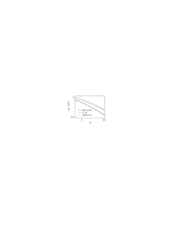
This modified PW2 form provides a much more drastic separation between the high– and low–density regime with respect to the original PW2 one. Such a separation is crucial to obtain a good fit which both reproduces the new QMC energies[13] at the highest densities and avoids undesired effects on the low–density regime (such as a negative coefficient for the $r_{s}^{-3/2}$ term). The parameters $A$, $\beta_{1}$, $\beta_{2}$, $\beta_{3}$ and $\alpha_{1}$ are fixed by imposing the high–density expansion of Eq. (21): $\alpha_{1}=C/A$, $\beta_{1}=0.5/A\exp(0.5B/A)$, $\beta_{2}=2A\beta_{1}^{2}$ and $\beta_{3}=0.5\beta_{1}(8\beta_{1}^{2}A^{4}-CB+DA)/A^{2}$. A best fit to new QMC data[13] gives for the 4 free parameters: $\alpha_{2}=5$, $\beta_{4}=45$, $\beta_{5}=32$, $\beta_{6}=12.7$. The resulting low–density expansion is $-0.39/r_{s}+0.99/r_{s}^{3/2}$. The maximum absolute error is 1.6 mRy, while the maximum relative error is 2.4%.

REFERENCES

- [1] E. Wigner, Phys. Rev. 46, 1002 (1934); Trans. Faraday Soc. 34, 678 (1938).
- [2] W. H. Young and N. H. March, Proc. R. Soc. London, Ser. A 256, 62 (1960); W. H.Young, Philos. Mag. 6, 371 (1961).
- [3] D. Pines and P. Nozières, Theory of Quantum Liquids (Benjamin, New York 1966).
- [4] see e.g. C. Kittel, Quantum Theory of Solids (Wiley, New York 1963), or J. M. Ziman, Principles of the Theory of Solids (Cambridge University Press 1969).
- [5] see e.g. W. A. Harrison, Pseudopotentials in the Theory of Metals (Benjamin, New York 1966).
- [6] D. R. Hamann, M. Schlüter, and C. Chiang, Phys. Rev. Lett. 43, 1494 (1979); G. B. Bachelet, D. R. Hamann, and M. Schlüter, Phys. Rev. B 26, 4199 (1982).
- [7] see e.g. K. S. Singwi and M. P.Tosi, Solid State Physics 36, 177 (1981); also, M. Hindgren and C.-O. Almbladh, Phys. Rev. B 56, 12832 (1997), and references therein.
- [8] D. M. Ceperley, Phys. Rev. B 18, 3126 (1978); D. M. Ceperley and B. J. Alder, Phys. Rev. Lett. 45, 566 (1980).
- [9] W. E. Pickett and J. Q. Broughton, Phys. Rev. B 48, 14859 (1993).
- [10] G. Ortiz and P. Ballone, Phys. Rev. B 50, 1391 (1994); ibid 56, 9970 (1997).
- [11] S. Moroni, D. M. Ceperley, and G. Senatore, Phys. Rev. Lett. 69, 1837 (1992); ibid 75, 826 (1995).
- [12] Y. Kwon, D. M. Ceperley, and R. M. Martin, Phys. Rev. B 58, 6800 (1998).
- [13] G. Ortiz, M. Harris, and P. Ballone, Phys. Rev. Lett. 82, 5317 (1999).
- [14] J. C. Slater, Phys. Rev. 81, 385 (1951).
- [15] P. Hohenberg and W. Kohn, Phys. Rev. 136, B864 (1964); W. Kohn and L. J. Sham, Phys. Rev. 140, A1133 (1965); N. D. Mermin, Phys. Rev. 137A, 1441 (1965); O. Gunnarsson and B. I. Lundqvist, Phys. Rev. B 13, 4724 (1976).
- [16] see e.g. R. G. Parr and W. Yang, Density-Functional Theory of Atoms and Molecules (Oxford Science 1989); for further examples of its present capabilities see R. Car, in Monte Carlo and Molecular Dynamics of Condensed Matter Systems, edited by K. Binder and G. Ciccotti, Conference Proceedings 49 (SIF, Bologna 1996); M. Boero, M. Parrinello, and K. Terakura, J. Am. Chem. Soc. 120, 2746 (1998).
- [17] O. Gunnarsson, M. Jonson, and B. I. Lundqvist, Phys. Rev. B 20, 3136 (1979).
- [18] J. P. Perdew and A. Zunger, Phys. Rev. B 23, 5048, (1981).
- [19] J. P. Perdew, Electronic Structure of Solids ’91, edited by P. Ziesche and H. Eschrig (Akademie Verlag, Berlin 1991); J. P. Perdew, K. Burke and Y. Wang, Phys. Rev. B 54, 16533 (1996); J. P. Perdew, K. Burke, and M. Ernzerhof, Phys. Rev. Lett. 77, 3865 (1996); ibid. 78, 1396 (1997).
- [20] O. Gunnarsson, M. Jonson, and B. I. Lundqvist, Phys. Lett. A 59, 177 (1976).
- [21] E. Chacón and P. Tarazona, Phys. Rev. B 37, 4013 (1988).
- [22] J. F. Dobson, J. Phys. C 4, 7877 (1992); ibid. J. Chem. Phys. 94, 4328 (1991); 98, 8870 (1993).
- [23] A. K. Rajagopal, J. C. Kimball, and M. Banerjee, Phys. Rev. B 18, 2339 (1978).
- [24] I. Yamashita and S. Ichimaru, Phys. Rev. B 29, 673 (1984).
- [25] V. Contini, G. Mazzone, and F. Sacchetti, Phys. Rev. B 33, 712 (1986).
- [26] C. Lee, W. Yang, and R. G. Parr, Phys. Rev. B 37, 785 (1988).
- [27] A. D. Becke, J. Chem. Phys. 88, 1053 (1988).
- [28] S. M. Valone, Phys. Rev. B 44, 1509 (1991).
- [29] J. P. Perdew and Y. Wang, Phys. Rev. B 46, 12947 (1992); ibid 56, 7018 (1997).
- [30] O. V. Gritsenko, A. Rubio, L. C. Balbás, and J. A. Alonso, Phys. Rev. A 47, 1811 (1993).
- [31] E. I. Proynov and D. R. Salahub, Phys. Rev. B 49, 7874 (1994).
- [32] in what follows we won’t be concerned with spatially nonuniform phases of jellium (although these phases are also of great interest: see e.g. J. A. Tuszyński, J. M. Dixon, and N. H. March, Phys. Rev. E 58, 318 (1998), or Refs. [1] and [13]).
- [33] J. C. Kimball, Phys. Rev. A 7, 1648 (1973); J. C. Kimball, J. Phys. A 8, 1513 (1975).
- [34] M. Hoffmann–Ostenhof, T. Hoffmann–Ostenhof, and H. Stremnitzer, Phys. Rev. Lett. 68, 3857 (1992).
- [35] N. Iwamoto, Phys. Rev. A 33, 1940 (1986).
- [36] S. Ueda, Prog. Theor. Phys. 26, 45 (1961).
- [37] Y. Wang and J. P. Perdew, Phys. Rev. B 44, 13298 (1991).
- [38] M. Gell–Mann and K. A. Brueckner, Phys. Rev. 106, 364 (1957).
- [39] P. Nozières and D. Pines, Phys. Rev. 111, 442 (1958).
- [40] N. H. March, Phys. Rev. 110, 604 (1958); P. N. Argyres, Phys. Rev. 154, 410 (1967); N. Iwamoto, Phys. Rev. B 38, 4277 (1988); L. Kleinman, Phys. Rev. B. 43, 3918 (1991).
- [41] J. P. Perdew and Y. Wang, Phys. Rev. B 45, 13244 (1992).
- [42] W. J. Carr, Jr. and A. A. Maradudin, Phys. Rev. 133 A371 (1964).
- [43] Y. Wang and J. P. Perdew, Phys. Rev. B 43, 8911 (1991).
- [44] G. G. Hoffman, Phys. Rev. B 45, 8730 (1992).
- [45] L. Onsager, L. Mittag, and M. J. Stephen, Ann. Phys. 18, 71 (1966).
- [46] T. Endo, M. Horiuchi, Y. Takada, and H. Yasuhara, Phys. Rev. B 59, 7367 (1999).
- [47] the gaussian cut–off used by several authors [10, 23, 24, 25, 29] in real or reciprocal space would, instead, give rise to unpleasant non–closed form espressions for the spherical Fourier transform of odd powers of [and/or ], since .
- [48] D. J. W. Geldart, Can. J. Phys. 45 3139 (1967); J. C. Kimball, Phys. Rev. B 14, 2371 (1976).
- [49] S. H. Vosko, L. Wilk, and M. Nusair, Can. J. Phys. 58, 1200 (1980).
- [50] V. C. Aguilera–Navarro, G. A. Baker, Jr., and M. de Llano, Phys. Rev. B 32, 4502 (1985).
- [51] we hear from J. P. Perdew that he and his collaborators are presently working on a better estimate for the spin resolution of the PW[29] pair–correlation function.
- [52] H. Yasuhara, Solid State Commun. 11, 1481 (1972).
- [53] V. A. Rassolov, J. A. Pople and M. A. Ratner, Phys. Rev. B 59, 15625 (1999).
- [54] R. A. Ferrel, Phys. Rev. Lett. 1, 443 (1958).
- [55] P. Ballone, private comunication.
- [56] H. Stoll, C. M. E. Pavlidou, and H. Preuss, Theor. Chim. Acta 49, 143 (1978); H. Stoll, E. Golka and H. Preuss, ibid. 55, 29 (1980).
- [57] R. Lobo, K. S. Singwi and M. P. Tosi, Phys. Rev. 186, 470 (1969); A. K. Rajagopal, J. Rath, and J. C. Kimball, Phys. Rev. B 7, 2657 (1973).
- [58] G. E. W. Bauer, Phys. Rev. B 27, 5912 (1983); A. Görling, M. Levy, and J. P. Perdew, Phys. Rev. B 47, 1167 (1993).