Effects of dilute nonmagnetic impurities on the ${\bf Q}=(\pi,\pi)$ spin-fluctuation spectrum
in YBa₂Cu₃O₇

Abstract

The effects of nonmagnetic impurities on the ${\bf Q}=(\pi,\pi)$ spin-fluctuation spectral weight ${\rm Im}\,\chi({\bf Q},\omega)$ are studied within the framework of the two-dimensional Hubbard model using the random phase approximation. In the first part of the paper, the effects of the nonmagnetic impurities on the magnetic susceptibility of the noninteracting ($U=0$) system, $\chi_{0}({\bf q},\omega)$, are calculated with the self-energy and the vertex corrections using various forms of the effective electron-impurity interaction. Here, the range and the strength of the impurity potential are varied as well as the concentration of the impurities. It is shown that the main effect of dilute impurities on $\chi_{0}({\bf Q},\omega)$ is to cause a weak smearing. In the second part, ${\rm Im}\,\chi({\bf Q},\omega)$ is calculated for the interacting system. Here, the calculations are concentrated on the processes which involve the impurity scattering of the spin fluctuations with finite momentum transfers. In order to make comparisons with the experimental data on the frequency dependence of ${\rm Im}\,\chi({\bf Q},\omega)$ in Zn substituted YBa₂Cu₃O₇, results are given for various values of the model parameters.

]

I Introduction and the Model

Zn substitution has been used as a probe of the electronic properties in the layered cuprates and has yielded important results. Small amount of Zn impurities lead to a strong suppression of $d$-wave pairing [1]. Resistivity measurements find that Zn impurities act as strong scatterers [2]. Local magnetic measurements on Zn substituted cuprates have also yielded valuable information [3, 4]. It has been found that within the presence of Zn impurities the uniform susceptibility of YBa₂Cu₃O_7-δ follows a Curie-like temperature dependence.

Inelastic neutron scattering experiments find that Zn impurities cause important changes in the ${\bf Q}\equiv(\pi,\pi)$ spin-fluctuation spectrum [5, 6, 7]. The experiments have been carried out for 2% [5] and 0.5% [6] Zn concentrations. It is found that even 0.5% Zn substitution in YBa₂Cu₃O₇ induces a peak in ${\rm Im}\,\chi({\bf Q},\omega)$ at $\omega=40$ meV in the normal state [6]. The $\omega$ width of the peak is about 10 meV and its width in momentum space is resolution limited. This peak becomes observable below $250^{\circ}$K and its intensity increases as $T$ is lowered without a discontinuity in its slope at $T_{c}=87^{\circ}$K. These results are quite different than those on pure YBa₂Cu₃O₇, where the peak is observed only in the superconducting state [8, 9, 10]. While in the case of 0.5% Zn substitution, no spectral weight is observed below $\sim 35$ meV, in the 2% Zn substituted sample there is significant amount of spectral weight down to 5 meV. In this case, there is also a broad peak at 35 meV. The momentum width of this peak is 0.5Å^-1, which is about twice that of the peak in the 0.5% Zn substituted and the pure samples. Hence, the two main features induced in ${\rm Im}\,\chi({\bf Q},\omega)$ in the normal state are the peak and the low frequency spectral weight observed in the 2% Zn substituted sample. Both of these features become observable already above $T_{c}$. The calculations reported in this article were carried out in order to investigate the origin of these two effects on the frequency dependence of ${\rm Im}\,\chi({\bf Q},\omega)$ in YBa₂Cu₃O₇ in the normal state.

Here, the results of diagrammatic calculations on the effects of nonmagnetic impurities on ${\rm Im}\,\chi({\bf Q},\omega)$ obtained using the framework of the two-dimensional Hubbard model will be given. In the first part of the paper, the effects of various types of effective electron-impurity interactions on the magnetic susceptibility of the noninteracting ($U=0$) system, $\chi_{0}({\bf Q},\omega)$, will be calculated. In this case, both the strength and the range of the impurity interaction, in addition to the concentration of impurities, will be varied. It will be found that in all these cases the main effect of impurity scattering is to cause a weak smearing of the structure in $\chi_{0}({\bf Q},\omega)$. Hence, at this level, if $\chi_{0}$ is used in an RPA expression, $\chi({\bf Q},\omega)=\chi_{0}({\bf Q},\omega)/(1-U\chi_{0}({\bf Q},\omega))$, then one obtains a smearing of ${\rm Im}\,\chi({\bf Q},\omega)$ by the impurity scattering rather than an enhancement as seen in the experiments. Here, it will be also noted that, for 2% impurity concentration, scatterings from an extended impurity potential could induce spectral weight at low frequencies.

In the next part of the paper, the effects of the processes where the spin fluctuations are scattered by the impurities with finite momentum transfers are calculated. This type of processes will be called the “umklapp” processes, since they involve the scattering of the spin fluctuations by the impurity potential with finite momentum transfers as in the case of the scattering of the spin fluctuations by a charge-density-wave field. In this part, the effects of the umklapp scatterings will be estimated by calculating the irreducible off-diagonal susceptibility $\chi_{0}({\bf q},{\bf q^{\prime}},\omega)$, where ${\bf q}\neq{\bf q^{\prime}}$, in the lowest order in the strength of the impurity potential. It will be seen that the important umklapp processes are the ones which involve the transfer of momentum $2{\bf k}_{F}$ to the spin fluctuations, and that they lead to a peak in ${\rm Im}\,\chi({\bf Q},\omega)$ at $\omega_{0}=2|\mu|$, where $\mu$ is the chemical potential. The underlying reason for this is a kinematic constraint which prohibits the creation of a particle-hole pair with center of mass momentum ${\bf q}=(\pi,\pi)-2{\bf k}_{F}$ and energy $\omega>\omega_{0}$. This constraint causes a nearly singular structure in $\chi_{0}({\bf Q},{\bf q},\omega)$ at $\omega=\omega_{0}$, which in turn leads to the peak in ${\rm Im}\,\chi({\bf Q},\omega)$ at $\omega_{0}$. This effect has been noted previously [11]. Here, results will be given for various sets of the model parameters in order to make comparisons with the experimental data. While in the pure system at low temperatures, the ${\bf Q}=(\pi,\pi)$ spin fluctuations are gapped below $\omega_{0}$, through this type of scatterings the ${\bf Q}=(\pi,\pi)$ spin fluctuations get mixed with the other wave vector components which are not gapped. This process can also lead to finite spectral weight for $\omega<\omega_{0}$. Comparisons with the experimental data suggest that the umklapp processes play an important role in determining the ${\bf Q}=(\pi,\pi)$ spin dynamics in Zn substituted YBa₂Cu₃O₇.

The starting point is the two-dimensional single-band Hubbard model given by

$$H=-t\sum_{\langle ij\rangle,\sigma}(c^{\dagger}_{i\sigma}c_{j\sigma}+c^{\dagger}_{j\sigma}c_{i\sigma})+U\sum_{i}c^{\dagger}_{i\uparrow}c_{i\uparrow}c^{\dagger}_{i\downarrow}c_{i\downarrow}$$ (1)

$$-\mu\sum_{i,\sigma}c^{\dagger}_{i\sigma}c_{i\sigma},$$ (2)

which will be used to model the spin fluctuations of the pure system. Here $c_{i\sigma}$ ($c^{\dagger}_{i\sigma}$) annihilates (creates) an electron with spin $\sigma$ at site $i$, $t$ is the near-neighbor hopping matrix element and $U$ is the onsite Coulomb repulsion. For simplicity, the hopping $t$, the lattice constant $a$ and $\hbar$ are set to 1.

Within the presence of an impurity, the magnetic susceptibility is defined by

$$\chi({\bf q},{\bf q^{\prime}},i\omega_{m})=\int_{0}^{\beta}d\tau\,e^{i\omega_{m}\tau}\langle m^{-}({\bf q},\tau)m^{+}({\bf q^{\prime}},0)\rangle,$$ (3)

where $m^{+}({\bf q})=N^{-1/2}\sum_{{\bf p}}c^{\dagger}_{{\bf p}+{\bf q}\uparrow}c_{{\bf p}\downarrow}$, $m^{-}({\bf q})=(m^{+}({\bf q}))^{\dagger}$, and $\omega_{m}=2m\pi T$. By letting $i\omega_{m}\rightarrow\omega+i\delta$, one obtains $\chi({\bf q},{\bf q^{\prime}},\omega)$. If one assumes that the effective interaction between an impurity and the electrons can be approximated by a static potential, then the RPA expression for the magnetic susceptibility becomes

$$\chi({\bf q},{\bf q}^{\prime},\omega) =\chi_{0}({\bf q},{\bf q}^{\prime},\omega)$$ (5)

$$+U\sum_{{\bf q}^{\prime\prime}}\chi_{0}({\bf q},{\bf q}^{\prime\prime},\omega)\chi({\bf q}^{\prime\prime},{\bf q}^{\prime},\omega),$$

where $\chi_{0}({\bf q},{\bf q^{\prime}},\omega)$ is the irreducible susceptibility dressed with the impurity scatterings. The off-diagonal ${\bf q}\neq{\bf q^{\prime}}$ terms of $\chi_{0}({\bf q},{\bf q^{\prime}},\omega)$ vanish for the pure system, but they are finite within the presence of impurity scattering. After obtaining $\chi({\bf q},{\bf q^{\prime}},\omega)$ from Eq. (5), the averaging over the impurity location can be done, which sets ${\bf q}={\bf q^{\prime}}$. $\chi({\bf q},{\bf q},\omega)$ obtained this way neglects the interactions between the impurities, and here it will be assumed that these can be ignored in the dilute limit. In the following, for simplicity, $\chi({\bf q},{\bf q},\omega)$ and $\chi_{0}({\bf q},{\bf q},\omega)$ will be denoted by $\chi({\bf q},\omega)$ and $\chi_{0}({\bf q},\omega)$, respectively.

In solving Eq. (5), if the off-diagonal terms are omitted, then one obtains

$$\chi({\bf q},\omega)={\chi_{0}({\bf q},\omega)\over 1-U\chi_{0}({\bf q},\omega)},$$ (6)

where $\chi_{0}({\bf q},\omega)$ is dressed with the impurity scatterings. In the next section, $\chi_{0}({\bf Q}=(\pi,\pi),\omega)$ will be calculated using various impurity potentials. In the third section, $\chi({\bf Q},\omega)$ will be calculated without omitting the off-diagonal terms in Eq. (5).

II Effects of the nonmagnetic impurities without the umklapp scatterings

In this part, the effects of dilute nonmagnetic impurities on the magnetic susceptibility of the noninteracting system will be calculated using various impurity potentials. The method used here for calculating $\chi_{0}({\bf Q},\omega)$ is similar to those used in Refs. [12, 13, 14]. Both the self-energy and the vertex corrections induced by the impurity scattering will be included [15, 16].

In Refs. [17, 18], it has been shown how the electronic correlations lead to an extended effective interaction between an impurity and the electrons. The extended nature of the effective impurity potential has been also emphasized in Ref. [19]. Assuming that it can be approximated by a static form, the potential due to an impurity at site ${\bf r}_{0}$ can be written as

$$V_{eff}=\sum_{\nu\alpha\sigma}V_{\nu\alpha}c^{\dagger}_{\nu\alpha\sigma}c_{\nu\alpha\sigma},$$ (7)

where $\nu$ denotes the distance from the impurity and $\alpha$ denotes the different partial wave components. The single-particle operators $c_{\nu\alpha\sigma}$ are given by

$$c_{\nu\alpha\sigma}=\sum_{{\bf d}_{\nu}}g_{\nu\alpha}({\bf d}_{\nu})c_{\sigma}({\bf r}_{0}+{\bf d}_{\nu}),$$ (8)

where ${\bf d}_{\nu}$ sums over the sites at a distance $\nu$ away from the impurity and $g_{\nu\alpha}({\bf d}_{\nu})$’s are the coefficients of the partial-wave components. In the following, an impurity interaction with a range of $\sqrt{2}$ lattice spacings, which includes the second near-neighbor site, will be considered. For simplicity, subscript $i$ will be used to denote both $\nu$ and $\alpha$.

Within the presence of impurity scattering, the single-particle Green’s function defined by

$$G({\bf p},\tau)=-\langle T_{\tau}c_{{\bf p}\sigma}(\tau)c^{\dagger}_{{\bf p}\sigma}(0)\rangle$$ (9)

is obtained from

$$G({\bf p},i\omega_{n}) =G_{0}({\bf p},i\omega_{n})$$ (11)

$$+n_{i}(G_{0}({\bf p},i\omega_{n}))^{2}\sum_{ij}g_{i}({\bf p})T_{ij}(i\omega_{n})g_{j}({\bf p}),$$

where $n_{i}$ is the concentration of the impurities and the Matsubara frequency $\omega_{n}=(2n+1)\pi T$. For an impurity potential with a range of $\sqrt{2}$ lattice spacings, the subscripts $i$ and $j$ vary from 1 to 9. The single-particle Green’s function of the pure system $G_{0}({\bf p},i\omega_{n})$ entering Eq. (11) is given by

$$G_{0}({\bf p},i\omega_{n})={1\over i\omega_{n}-\varepsilon_{\bf p}}$$ (12)

where the single-particle dispersion relation is

$$\varepsilon_{\bf p}=-2t(\cos{p_{x}}+\cos{p_{y}})-\mu.$$ (13)

The terms contributing to $G({\bf p},i\omega_{n})$ are illustrated diagrammatically in Fig. 1(a). In Eq. (11), $T_{ij}(i\omega_{n})$ is the impurity-scattering $t$-matrix and $g_{i}({\bf p})$’s are the form factors which are given by

$$g_{i}({\bf p})=\sum_{{\bf d}_{\nu}}g_{\nu\alpha}({\bf d}_{\nu})e^{i{\bf p}\cdot{\bf d}_{\nu}},$$ (14)

where $i$ denotes $(\nu,\alpha)$. The first five of the nine form factors used here are

$$g_{0s}({\bf p}) =1$$ (15)

$$g_{1s}({\bf p}) =\cos{p_{x}}+\cos{p_{y}}$$ (16)

$$g_{1p_{x}}({\bf p}) =\sin{p_{x}}$$ (17)

$$g_{1p_{y}}({\bf p}) =\sin{p_{y}}$$ (18)

$$g_{1d}({\bf p}) =\cos{p_{x}}-\cos{p_{y}}$$ (19)

with similar expressions for the remaining $\alpha=\sqrt{2}$ components having $s$, $p_{x}$, $p_{y}$ and $d$-wave symmetries. The $t$-matrix $T_{ij}(i\omega_{n})$ is obtained by solving

$$T_{ij}(i\omega_{n})=\delta_{ij}V_{i}+V_{i}\sum_{\ell}F_{i\ell}(i\omega_{n})T_{\ell j}(i\omega_{n}),$$ (20)

where

$$F_{ij}(i\omega_{n})={1\over N}\sum_{\bf p}g_{i}({\bf p})G_{0}({\bf p},i\omega_{n})g_{j}({\bf p}).$$ (21)

In order to calculate $\chi_{0}({\bf Q},i\omega_{m})$, the irreducible interaction $\Gamma^{0}$ in the particle-hole channel due to impurity scattering is needed. In Fig. 1(b), $\Gamma^{0}$ is illustrated diagrammatically and the corresponding expression is

$$\Gamma^{0}_{ii^{\prime},jj^{\prime}} ({\bf p},{\bf p^{\prime}},i\omega_{n},i\omega_{m})=-n_{i}g_{i}({\bf p})g_{i^{\prime}}({\bf p}+{\bf Q})$$ (23)

$$\times T_{ij}(i\omega_{n})T_{i^{\prime}j^{\prime}}(i\omega_{n}+i\omega_{m})g_{j}({\bf p^{\prime}})g_{j^{\prime}}({\bf p^{\prime}}+{\bf Q}).$$

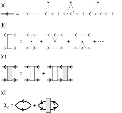
FIG. 1.: (a) Feynman diagrams for the single-particle Green’s function dressed with the impurity scatterings. (b) Irreducible vertex $\Gamma^{0}$ in the particle-hole channel arising from the impurity scattering. (c) Reducible vertex $\Gamma$ in the particle-hole channel given in terms of $\Gamma^{0}$. (d) Irreducible magnetic susceptibility $\chi_{0}({\bf Q},i\omega_{m})$ dressed with the impurity-induced self-energy and vertex corrections.

Here, $\Gamma^{0}$ is evaluated with the center-of-mass momentum ${\bf Q}\equiv(\pi,\pi)$. Next, the reducible vertex in the particle-hole channel is obtained by solving

$$\Gamma {}_{ii^{\prime},jj^{\prime}}({\bf p},{\bf p^{\prime}},i\omega_{n},i\omega_{m})=\Gamma^{0}_{ii^{\prime},jj^{\prime}}({\bf p},{\bf p^{\prime}},i\omega_{n},i\omega_{m})$$ (26)

$$-\sum_{\ell\ell,ss^{\prime}}{1\over N}\sum_{\bf k}\Gamma^{0}_{ii^{\prime},\ell\ell^{\prime}}({\bf p},{\bf k},i\omega_{n},i\omega_{m})G({\bf k},i\omega_{n})$$

$$\times G({\bf k}+{\bf Q},i\omega_{n}+i\omega_{m})\Gamma_{ss^{\prime},jj^{\prime}}({\bf k},{\bf p^{\prime}},i\omega_{n},i\omega_{m}),$$

which is illustrated in Fig. 1(c). Here, it is noted that $\Gamma^{0}$ is calculated using the bare single-particle Green’s function $G_{0}$, while $\Gamma$ is calculated using the Green’s function dressed with the impurity scatterings. This is necessary in order to prevent double-counting [16]. In terms of the reducible vertex, $\chi_{0}({\bf Q},i\omega_{m})$ is given by

$$\chi_{0}({\bf Q},i\omega_{m})=\overline{\chi} {}_{0}({\bf Q},i\omega_{m})$$ (27)

$$-T\sum_{i\omega_{n}}{1\over N}\sum_{\bf p}{1\over N} \sum_{\bf p^{\prime}}G({\bf p}+{\bf Q},i\omega_{n}+i\omega_{m})G({\bf p},i\omega_{n})$$ (28)

$$\times\sum_{ii^{\prime},jj^{\prime}}\Gamma_{ii^{\prime},jj^{\prime}} ({\bf p},{\bf p^{\prime}},i\omega_{n},i\omega_{m})G({\bf p^{\prime}}+{\bf Q},i\omega_{n}+i\omega_{m})$$ (30)

$$\times G({\bf p^{\prime}},i\omega_{n}).$$

Here, $\overline{\chi}_{0}({\bf Q},i\omega_{m})$ includes only the impurity induced self-energy corrections, and it is given by

$$\overline{\chi}_{0}({\bf Q},i\omega_{m})=-{T\over N}\sum_{{\bf p},i\omega_{n}}G({\bf p}+{\bf Q},i\omega_{n}+i\omega_{m})$$ (31)

$$\times G({\bf p},i\omega_{n}).$$ (32)

These results in terms of the Matsubara frequencies are analytically continued to the real frequency axis by the Pade approximation. In the following, the results on $\chi_{0}({\bf Q},\omega)$ obtained this way will be compared with the Lindhard susceptibility of the pure system,

$$\chi^{L}_{0}({\bf Q},\omega)={1\over N}\sum_{\bf p}{f(\varepsilon_{{\bf p}+{\bf Q}})-f(\varepsilon_{\bf p})\over\omega-(\varepsilon_{{\bf p}+{\bf Q}}-\varepsilon_{\bf p})+i\delta}.$$ (33)

Figure 2 shows results obtained using a strongly attractive onsite impurity potential $V_{0}=-20$ and an impurity concentration of $n_{i}=0.02$. In addition, here filling $\langle n\rangle=0.875$ and temperature $T=0.02$ are used. In Fig. 2(a), $\chi_{0}({\bf Q},i\omega_{m})$ versus $\omega_{m}$ is shown. Also shown in this figure are $\overline{\chi}_{0}({\bf Q},i\omega_{m})$, which does not include the impurity vertex corrections, and the Lindhard susceptibility $\chi_{0}^{L}({\bf Q},i\omega_{m})$ of the pure system. Figures 2(b) and (c) show the corresponding real and imaginary parts obtained by the Pade analytic continuation. Here, one observes that the impurity-induced self-energy corrections suppress $\chi_{0}({\bf Q},i\omega_{m})$ and smear the structure in $\chi_{0}({\bf Q},\omega)$. For instance, the hump in ${\rm Re}\,\chi_{0}^{L}({\bf Q},\omega)$ at $\omega\approx 2|\mu|=0.48$ is smeared by the self-energy corrections, but when the vertex corrections are included, the effect of the

FIG. 2.: Results on (a) $\chi_{0}({\bf Q},i\omega_{m})$ versus $\omega_{m}$, (b) ${\rm Re}\,\chi_{0}({\bf Q},\omega)$ versus $\omega$ and (c) ${\rm Im}\,\chi_{0}({\bf Q},\omega)$ versus $\omega$ for an onsite impurity potential with $V_{0}=-20$ and impurity concentration $n_{i}=0.02$. These results were obtained for $\langle n\rangle=0.875$ and $T=0.02$.

self-energy corrections is nearly canceled. This hump is because of a logarithmic singularity in ${\rm Re}\,\chi_{0}({\bf Q},\omega)$ at $T=0$ originating from the dynamic nesting of the Fermi surface. In a real system, the deviations from the simple tight-binding model which has only near-neighbor hoppings would lead to a suppression of this hump. In addition, the scattering of the single-particle excitations by the spin-fluctuations would suppress it also. In Figs. 2(b) and (c), the difference between the solid and the dotted lines is of order the resolution of the Pade analytic continuation. These calculations were repeated using $n_{i}=0.005$ instead of $n_{i}=0.02$, in which case the difference between $\chi_{0}$ and $\chi_{0}^{L}$ becomes even smaller (not shown here).

Figure 3 shows results also for $n_{i}=0.02$ and an onsite impurity potential but now with $V_{0}=-1$. One observes that in this case the impurities have a stronger effect on $\chi_{0}$. In addition, it is noted that ${\rm Re}\,\chi_{0}({\bf Q},\omega)$ for $\omega\sim 0.5$ is suppressed, and ${\rm Re}\,\chi_{0}({\bf Q},\omega\sim 0)$ gets enhanced by a small amount. Among the various forms tried for the impurity potential, this is the only case where an enhancement of $\chi_{0}({\bf Q},\omega)$ by the impurity scatterings has been obtained. This effect is due to the enhancement of the single-particle density of states at the impurity site by the attractive potential. The enhancement of ${\rm Re}\,\chi_{0}({\bf Q},\omega\sim 0)$ at small frequencies could lead to some enhancement of the low-frequency antiferromagnetic spin

FIG. 3.: Results similar to those in Fig. 2 but for $V_{0}=-1$.

fluctuations for a system with a large Stoner factor. However, it is seen that ${\rm Re}\,\chi_{0}({\bf Q},\omega)$ for $\omega$ near $\omega_{0}=2|\mu|$ is suppressed, and actually it would not be possible to explain the peak in the neutron scattering data with these results. This calculation was repeated using $V_{0}=1$, and a suppresion of ${\rm Re}\,\chi_{0}({\bf Q},\omega)$ was obtained due to the depletion of the single-particle density of states (not shown here).

Figure 4 shows results on $\chi_{0}$ obtained using an extended impurity potential for $n_{i}=0.02$ and 0.005. These results were obtained for a potential with a range of $\sqrt{2}$ lattice spacings and with the following parameters: $V_{0s}=-20$, $V_{1\alpha}=0.5$ and $V_{\sqrt{2}\alpha}=-0.25$ where $\alpha$ denotes the $s$, $p_{x}$, $p_{y}$ and $d$-wave components. These values for $V_{\nu\alpha}$’s are comparable to those obtained in Ref. [18]. The calculations were repeated using various other values for the $V_{\nu\alpha}$’s, and it has been found that small changes in $V_{\nu\alpha}$’s do not change the results shown here significantly. For instance, increasing $V_{\nu\alpha}$’s by 50% does not change the conclusions of this section. In Fig. 4, it is seen that for $n_{i}=0.02$ an extended potential leads to significant smearing of the structure in $\chi_{0}({\bf Q},\omega)$. In this case, the hump in ${\rm Re}\,\chi_{0}({\bf Q},\omega)$ is rounded off, and spectral weight is induced for $\omega<\omega_{0}$. Hence, comparing with Fig. 2, one observes that while an onsite impurity potential

FIG. 4.: Results similar to those in Fig. 2 but for an extended potential with the following set of parameters: $V_{0s}=-20$, $V_{1\alpha}=0.5$ and $V_{\sqrt{2}\alpha}=-0.5$. Here results are given for both $n_{i}=0.02$ and 0.005.

does not lead to spectral weight for $\omega<\omega_{0}$, an extended potential induces spectral weight in the gap. Also shown in Fig. 4 are the results for $n_{i}=0.005$, in which case the effect of the impurities on $\chi_{0}({\bf Q},\omega)$ is weaker. The fact that 0.5% impurities induce less spectral weight in the gap compared to the 2% case is consistent with the neutron scattering data by Refs. [5, 6]. However, even for $n_{i}=0.02$, the amount of the spectral weight induced in the gap is small. In the next section, it will be seen that the umklapp processes could also contribute to ${\rm Im}\,\chi({\bf Q},\omega)$ for $\omega<\omega_{0}$.

From the results presented here, one observes that if $\chi_{0}({\bf Q},\omega)$ computed in this section is used in Eq. (6), which omits the umklapp scatterings, then one would only obtain a smearing of ${\rm Im}\,\chi({\bf Q},\omega)$ by the impurities. Hence, it would not be possible to explain how 0.5% Zn impurities induce a peak in ${\rm Im}\,\chi({\bf Q},\omega)$ in the normal state of YBa₂Cu₃O₇. In the next section, the effects of the impurity scatterings with finite momentum transfers will be taken into account.

III Effects of the impurity induced umklapp scatterings

Here, ${\rm Im}\,\chi({\bf Q},\omega)$ will be calculated without omitting the off-diagonal components in Eq. (5). These off-diagonal terms will be calculated in the lowest order in the strength of the impurity potential, as illustrated diagrammatically in Fig. 5(a). In the previous section, it was found that 0.5% and 2% impurities cause only a weak smearing of $\chi_{0}({\bf Q},\omega)$. For this reason, the diagonal components of Eq. (5) will be approximated by the Lindhard susceptibility $\chi_{0}^{L}$. This will not change the nearly singular contribution originating from the umklapp scatterings at $\omega\approx\omega_{0}$. The expression for $\chi_{0}({\bf Q},{\bf q},i\omega_{m})$ corresponding to the diagrams shown in Fig. 5(a) is

$$\chi_{0}({\bf Q},{\bf q},i\omega_{m})=-V_{0}{T\over N} \sum_{{\bf p},i\omega_{n}}\bigg{\{}G_{0}({\bf p}+{\bf Q},i\omega_{n}+i\omega_{m})$$ (34)

$$\times G_{0}({\bf p},i\omega_{n}) G_{0}({\bf p}+{\bf Q}-{\bf q},i\omega_{n})$$ (35)

$$+G_{0}({\bf p},i\omega_{n}) G_{0}({\bf p}+{\bf q},i\omega_{n}+i\omega_{m})$$ (36)

$$\times G_{0}({\bf p}+{\bf Q},i\omega_{n}+i\omega_{m})\bigg{\}}.$$ (37)

Here ${\bf Q}\equiv(\pi,\pi)$ and ${\bf q}={\bf Q}-{\bf Q^{*}}$, where ${\bf Q^{*}}$ is the momentum transferred during the scattering from the impurity. Upon carrying out the summation over $i\omega_{n}$ in Eq. (34) and letting $i\omega_{m}\rightarrow\omega+i\delta$, one obtains

$$\chi_{0}({\bf Q},{\bf q},\omega) =A({\bf Q},{\bf q},\omega)+A^{*}({\bf Q},{\bf q},-\omega)$$ (39)

$$+B({\bf Q},{\bf q},\omega)-B^{*}({\bf Q},{\bf q},-\omega),$$

where “*” stands for complex conjugation, and $A$ and $B$ are given by

$$A({\bf Q},{\bf q},\omega)=-{V_{\bf k}\over N}\sum_{\bf p}\bigg{\{}{f(\varepsilon_{{\bf p}+{\bf Q^{*}}})\over\omega-(\varepsilon_{{\bf p}+{\bf Q}}-\varepsilon_{{\bf p}+{\bf Q^{*}}})+i\delta}$$ (40)

$$-{f(\varepsilon_{\bf p})\over\omega-(\varepsilon_{{\bf p}+{\bf Q}}-\varepsilon_{\bf p})+i\delta}\bigg{\}}{1\over\varepsilon_{{\bf p}+{\bf Q^{*}}}-\varepsilon_{\bf p}}$$ (41)

$$B({\bf Q},{\bf q},\omega)=-{V_{\bf k}\over N}\sum_{\bf p}{1\over\varepsilon_{{\bf p}+{\bf Q^{*}}}-\varepsilon_{\bf p}}$$ (42)

$$\times{f(\varepsilon_{{\bf p}+{\bf Q^{*}}})\over(\omega-(\varepsilon_{{\bf p}+{\bf Q}}-\varepsilon_{{\bf p}+{\bf Q^{*}}})+i\delta)(\omega-(\varepsilon_{{\bf p}+{\bf Q}}-\varepsilon_{\bf p})+i\delta)}.$$ (43)

A general form for the effective interaction between the electrons and an impurity located at site ${\bf r}_{0}$ is given by

$$V_{eff}={1\over N}\sum_{{\bf k}}e^{i{\bf k}\cdot{\bf r}_{0}}V_{{\bf k}}\sum_{{\bf p},\sigma}c^{\dagger}_{{\bf p}+{\bf k}\sigma}c_{{\bf p}\sigma}.$$ (44)

Below, it will be seen that for ${\bf Q^{*}}$ near $2{\bf k}_{F}$, $\chi_{0}({\bf Q},{\bf q},\omega)$ has a nearly singular structure at $\omega\approx\omega_{0}$, while for ${\bf Q^{*}}$ away from $2{\bf k}_{F}$, $\chi_{0}({\bf Q},{\bf q},\omega)$ is a smooth function of $\omega$ with a small amplitude. Hence, $\chi({\bf Q},\omega)$ will be calculated using only the $\pm{\bf Q^{*}}$ components of the effective impurity interaction,

$$V_{0}\sum_{{\bf p}\sigma}(c^{\dagger}_{{\bf p}+{\bf Q^{*}}\sigma}c_{{\bf p}\sigma}+c^{\dagger}_{{\bf p}-{\bf Q^{*}}\sigma}c_{{\bf p}\sigma}),$$ (45)

where $V_{0}=V_{\bf Q^{*}}$ is taken as a parameter. This is necessary, since, in order to have sufficient frequency resolution, the calculation needs to be carried out on a large lattice, which is difficult to do using directly Eq. (44). Furthermore, the detailed ${\bf k}$ dependence of $V_{\bf k}$ is not known, especially for ${\bf k}$ near $2{\bf k}_{F}$. The scattering of a quasiparticle with ${\bf Q^{*}}=2{\bf k}_{F}$ momentum transfer is sketched in the Brillouin zone in Fig. 5(b). Using the interaction given

FIG. 5.: (a) Feynman diagrams for the lowest-order terms contributing to the off-diagonal irreducible susceptibility $\chi_{0}({\bf Q},{\bf q},\omega)$. (b) Sketch in the Brillouin zone of a quasiparticle scattering process where momentum $2{\bf k}_{F}$ is transferred.

in Eq. (45), one obtains for $\chi({\bf Q},\omega)$,

$$\chi({\bf Q} ,\omega)=\Big{\{}\chi^{L}_{0}({\bf Q},\omega)(1-U\chi^{L}_{0}({\bf q},\omega))$$ (48)

$$+4U(\chi_{0}({\bf Q},{\bf q},\omega))^{2}\Big{\}}\times\Big{\{}(1-U\chi^{L}_{0}({\bf Q},\omega))$$

$$\times(1-U\chi^{L}_{0}({\bf q},\omega))-4(U\chi_{0}({\bf Q},{\bf q},\omega))^{2}\Big{\}}^{-1},$$

where ${\bf q}={\bf Q}-{\bf Q^{*}}$. Here, the factor of 4 multiplying $(\chi_{0}({\bf Q},{\bf q},\omega))^{2}$ is to take into account the scatterings with momentum transfers $(\pm Q^{*},\mp Q^{*})$ in addition to $(\pm Q^{*},\pm Q^{*})$, where ${\bf Q^{*}}=(Q^{*},Q^{*})$.

In the following, results will be shown for $\langle n\rangle=0.86$ and $T=0.05$, in which case $\omega_{0}=2|\mu|\approx 0.55$. Figure 6(a) shows the real and the imaginary parts of $\chi_{0}({\bf Q},{\bf q},\omega)$ for ${\bf Q^{*}}=2{\bf k}_{F}$. Here, the Fermi wave vector ${\bf k}_{F}$ has been taken along (1,1) for simplicity. In evaluating $\chi({\bf Q},\omega)$ with Eq. (48), the Lindhard susceptibilities $\chi_{0}^{L}({\bf Q},\omega)$ and $\chi_{0}^{L}({\bf q}={\bf Q}-{\bf Q^{*}},\omega)$ are also used and, hence, they are plotted in Figures 6(b) and (c). Here, one notes the similarity between the $\omega$ dependence of $\chi_{0}({\bf Q},{\bf q},\omega)$ and $\chi_{0}^{L}({\bf q}={\bf Q}-{\bf Q^{*}},\omega)$. Both have vanishing spectral weight for $\omega>\omega_{0}$ because of kinematic constraints.

In Fig. 7, ${\rm Im}\,\chi({\bf Q},\omega)$ versus $\omega$ obtained from Eq. (48) by using the results of Fig. 6 are shown for different values of $U$. The solid lines are for $V_{0}=0.05$ and the dashed lines are for $V_{0}=0$ corresponding to the pure case. Here,

FIG. 6.: Frequency dependence of (a) $\chi_{0}({\bf Q},{\bf q},\omega)$ (b) $\chi^{L}_{0}({\bf Q},\omega)$ and (c) $\chi^{L}_{0}({\bf q},\omega)$. Here ${\bf q}={\bf Q}-{\bf Q^{*}}$ and ${\bf Q^{*}}=2{\bf k}_{F}$. These results were obtained for $\langle n\rangle=0.86$ and $T=0.05$.

FIG. 7.: ${\rm Im}\,\chi({\bf Q},\omega)$ versus $\omega$ for (a) $U=1.5$, (b) $U=1.7$, and (c) $U=2.0$. These results were for $V_{0}=0.05$ and 0. If the value of $V_{0}$ is increased to 0.06, the sharp peak at $\omega_{0}\approx 0.55$ diverges.

it is seen that a peak is induced at $\omega_{0}\approx 0.55$ by turning on $V_{0}$. One also observes that as $U$ is increased, a hump develops below the peak. This is because of the RPA enhancement of $\chi$ in the pure case. In a real system, it is expected that this hump will be smaller because of the band-structure effects and the damping of the quasiparticles by the spin fluctuations. In Fig. 8, it is also seen that the impurity contribution to the low frequency part of ${\rm Im}\,\chi({\bf Q},\omega)$ increases as $U$ is increased. In addition, in Fig. 6(c) it was seen that $\chi_{0}({\bf q}={\bf Q}-2{\bf k}_{F},\omega)$ has sharp structure near $\omega_{0}$, but this is not responsible for producing the peak in ${\rm Im}\,\chi({\bf Q},\omega)$. For instance, taking out the factor of $(1-U\chi_{0}^{L}({\bf q},\omega))$ from both the numerator and the denominator in Eq. (48) does not change the structure of ${\rm Im}\,\chi({\bf Q},\omega)$.

Next, in order to have a better understanding of these results, a sketch of the important wave vectors and frequencies are given in the ${\bf q}$-$\omega$ plane in Fig. 8. Here, ${\bf Q}=(\pi,\pi)$, and ${\bf q}$ and $2{\bf k}_{F}$ are taken along (1,1). The vertical dashed line denotes ${\bf q}={\bf Q}-2{\bf k}_{F}$ and the horizontal dashed line is for $\omega_{0}=2|\mu|$. The shaded area represents the region where ${\rm Im}\,\chi_{0}^{L}({\bf q},\omega)\neq 0$ at $T=0$. Here, one observes that the ${\bf Q^{*}}=2{\bf k}_{F}$ scattering of the ${\bf Q}=(\pi,\pi)$ spin fluctuations will lead to a mixing with the ${\bf q}={\bf Q}-2{\bf k}_{F}$ component of the spin fluctuations, which has spectral weight only for $\omega<\omega_{0}$. A general

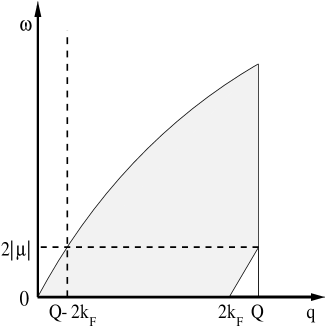
FIG. 8.: Sketch in ${\bf q}-\omega$ plane of the important wave vectors and frequencies (not to scale). The vertical dashed line denotes ${\bf q}={\bf Q}-2{\bf k}_{F}$ where ${\bf Q}=(\pi,\pi)$ and the horizontal dashed line denotes $\omega_{0}=2|\mu|$. The shaded area represents the region where ${\rm Im}\,\chi^{L}_{0}({\bf q},\omega)\neq 0$ at $T=0$. Here ${\bf q}$ and $2{\bf k}_{F}$ were taken along $(1,1)$.

impurity potential such as Eq. (44) would lead to a mixing with all wave vectors. Hence, the umklapp processes could also contribute to ${\rm Im}\,\chi({\bf Q},\omega)$ for $\omega<\omega_{0}$, in addition to the results seen in the previous section.

In order to show that the nearly singular $\omega$ dependence of $\chi_{0}({\bf Q},{\bf q},\omega)$ occurs only for ${\bf Q^{*}}\approx 2{\bf k}_{F}$, in Fig. 9 results on $\chi_{0}({\bf Q},{\bf q},\omega)/V_{0}$ are shown for various values of ${\bf Q^{*}}$. As seen in Fig. 9(a), for ${\bf Q^{*}}=1.02(2{\bf k}_{F})$, there is a sharp structure in $\chi_{0}({\bf Q},{\bf q},\omega)$ at $\omega$ less than $\omega_{0}$, while for ${\bf Q^{*}}=0.98(2{\bf k}_{F})$, this occurs at $\omega>\omega_{0}$. As ${\bf Q^{*}}$ moves away from $2{\bf k}_{F}$, the position of the structure in $\chi_{0}({\bf Q},{\bf q},\omega)$ shifts away from $\omega_{0}$ and its amplitude decreases. In Figs. 9(b) and (c), results on ${\rm Re}\,\chi_{0}({\bf Q},{\bf q},\omega)/V_{0}$ versus $\omega$ are shown for ${\bf Q^{*}}$ along (1,1) and (1,0), respectively. Here, ${\rm Im}\,\chi_{0}({\bf Q},{\bf q},\omega)/V_{0}$ is not shown since it is a smooth function of $\omega$ with amplitude less than 0.05. In these figures, it is seen that the magnitude of $\chi_{0}({\bf Q},{\bf q},\omega)$ at $\omega\approx\omega_{0}$ is considerably smaller when ${\bf Q^{*}}$ is away from $2{\bf k}_{F}$. This supports the use of only the ${\bf Q^{*}}$ component of $V_{eff}$ in solving for $\chi({\bf Q},\omega)$. If a general potential such as Eq. (44) instead of Eq. (45) were used in solving for $\chi({\bf Q},\omega)$, then the peak in ${\rm Im}\,\chi({\bf Q},\omega)$ would again occur at $\omega_{0}$ but with a broadened width because of the contributions originating from scatterings with ${\bf Q^{*}}$ slightly away from $2{\bf k}_{F}$.

In Fig. 7, one notes that the line shape of the peak depends on the value of $U$. For $U=1.5$ and 1.7, the peak is asymmetric; there is a dip below the peak. For $U=2.0$, the dip is not observed. In order to have a better understanding of this, further results on the line shape are shown in Figures 10(a) and (b) for $U=1.7$ and 2.0, respectively. In these figures, if the value of $V_{0}$ is increased to 0.06, the peak at $\omega_{0}$ diverges. Also shown here in Fig. 10(c) is the quantity

FIG. 9.: (a) $\chi_{0}({\bf Q},{\bf q},\omega)/V_{0}$ versus $\omega$ for different values of ${\bf Q^{*}}$ near $2{\bf k}_{F}$ along (1,1). Here, the numbers next to the curves indicate the magnitude of ${\bf Q^{*}}$ in units of $2k_{F}$. The solid and the dotted curves represent the real and the imaginary parts. In (b) and (c), results on ${\rm Re}\,\chi_{0}({\bf Q},{\bf q},\omega)/V_{0}$ versus $\omega$ are plotted for ${\bf Q^{*}}$ away from $2{\bf k}_{F}$.

$$\gamma(\omega)=4U^{2}(\chi_{0}({\bf Q},{\bf q},\omega))^{2},$$ (49)

which enters Eq. (48). For $U=1.7$, the system is away from the magnetic instability and, in this case, ${\rm Re}\,\gamma(\omega)$ has a stronger effect than the imaginary part. While for $\omega>\omega_{0}$, ${\rm Re}\,\gamma(\omega)$ leads to a stronger RPA enhancement of ${\rm Im}\,\chi({\bf Q},\omega)$, for $\omega<\omega_{0}$ it suppresses ${\rm Im}\,\chi({\bf Q},\omega)$. On the other hand, for $U=2$, where $1-U{\rm Re}\,\chi_{0}^{L}({\bf Q},\omega)$ is small, the pure system is already close to the magnetic instability and $U{\rm Im}\,\chi_{0}^{L}({\bf Q},\omega)$ acts as a damping of the RPA enhancement. In this case, ${\rm Im}\,\gamma(\omega)$ becomes more important and it leads to the peak in ${\rm Im}\,\chi({\bf Q},\omega)$ by suppressing the damping of the RPA enhancement. Possibly, this is the case more applicable to YBa₂Cu₃O₇.

The results seen in Fig. 10 were obtained using a finite broadening $\delta=0.001$ in Eqs. (33), (40) and (42). For comparison, results obtained using $\delta=0.01$ are shown in Fig. 11. In this case, the structure in $\gamma(\omega)$ and the peak in ${\rm Im}\,\chi({\bf Q},\omega)$ are broader. It is also seen that the integrated spectral weight in the peak increases with $\delta$ for $U=2$. If $\delta$ is increased further, the width of the peak in ${\rm Im}\,\chi({\bf Q},\omega)$ for $U=2$ continues to increase (not shown here). It is noted that the scattering of the quasiparticles

FIG. 10.: ${\rm Im}\,\chi({\bf Q},\omega)$ versus $\omega$ for different values of $V_{0}$, and for (a) $U=1.7$ and (b) $U=2$. (c) $\gamma(\omega)$ versus $\omega$ for $V_{0}=0.05$ and $U=2.0$. These results were obtained for $\delta=0.001$.

by the spin fluctuations could have an effect similar to that of the finite broadening $\delta$ used here. This could be another reason for why the peak observed in ${\rm Im}\,\chi({\bf Q},\omega)$ of Zn substituted samples has a finite width. So, in these figures it is observed that the quantitative features of the changes induced by the umklapp processes depend on the model parameters.

IV DISCUSSION

In summary, the effects of dilute nonmagnetic impurities on the frequency dependence of ${\rm Im}\,\chi({\bf Q},\omega)$ have been studied. These calculations were motivated by the neutron scattering data of Refs. [5, 6] on 2% and 0.5% Zn substituted YBa₂Cu₃O₇. The origin of the peak and of the low-frequency spectral weight induced by the impurities are the two issues which have been addressed in this paper.

In pure YBa₂Cu₃O₇, a resonant peak is observed only in the superconducting state at $\omega=41$ meV [8, 9, 10]. The width of this peak is resolution limited as opposed to that observed in the Zn substituted samples. The theories attribute the resonant peak of the pure sample to instabilities in the particle-particle [20, 21] or the magnetic channels [22, 23, 24]. The calculations presented here

FIG. 11.: Results similar to those shown in Fig. 10 but for $\delta=0.01$ and different values of $V_{0}$.

show how a peak in ${\rm Im}\,\chi({\bf Q},\omega)$ of Zn substituted YBa₂Cu₃O₇ could arise from the magnetic channel in the normal state. However, clearly, the contributions to the peak from other channels are not ruled out.

The calculations have been carried out first without taking into account the umklapp scattering of the spin fluctuations. Here, the influence of the range of the impurity potential on $\chi_{0}({\bf Q},\omega)$ has been studied. When a strongly attractive onsite impurity potential is used, it has been found that 2% impurities have a negligible effect on $\chi_{0}({\bf Q},\omega)$. This is in agreement with the calculations of Ref. [14] in the unitary limit for an onsite potential. When an extended impurity potential is used with parameters similar to those obtained from the exact diagonalization calculations [18], 2% impurities lead to the smearing of $\chi_{0}({\bf Q},\omega)$ inducing spectral weight below $\omega_{0}$. However, for 0.5% impurities a negligible effect is found.

In the third section, the effects of the processes where the spin fluctuations scatter from the impurities with finite momentum transfers were taken into account. It has been shown that the scatterings of the spin fluctuations with momentum transfers ${\bf Q^{*}}\approx 2{\bf k}_{F}$ lead to a peak in ${\rm Im}\,\chi({\bf Q},\omega)$ at $\omega\approx\omega_{0}=2|\mu|$. Here, the dependence of the impurity induced changes on the model parameters have been studied in order to make comparisons with the neutron scattering data. For instance, it was seen that the line shape of the peak depends on the model parameters. When the parameters are such that the Stoner enhancement is small, a dip is observed below the peak. On the other hand, when $1-U{\rm Re}\,\chi_{0}({\bf Q},\omega)$ is small, the dip is not observed and the $2{\bf k}_{F}$ scatterings lead to a peak in ${\rm Im}\,\chi({\bf Q},\omega)$ by suppressing the damping of the RPA enhancement. In addition, in this case, the width of the peak increases with the broadening of the single-particle excitations. It has been also found that the impurity scatterings with finite momentum transfers could lead to spectral weight below $\omega_{0}$. Hence, along with the results seen in the second section, the umklapp processes could also play a role in inducing the low frequency spectral weight observed in 2% Zn substituted YBa₂Cu₃O₇ [5].

The general features of the impurity induced changes in ${\rm Im}\,\chi({\bf Q},\omega)$ calculated here appear to be in agreement with the experimental data on Zn substituted YBa₂Cu₃O₇. However, in obtaining these results the Coulomb correlations were treated within RPA and $\chi_{0}({\bf Q},{\bf q},\omega)$ has been calculated in the lowest order in the strength of the impurity potential. Furthermore, a static effective impurity potential was used. If the results presented here are supported by higher order calculations, then it would mean that a contribution to the peak observed in ${\rm Im}\,\chi({\bf Q},\omega)$ could arise from the magnetic channel. Furthermore, in this case, the experimental data of Refs. [5, 6] would mean that a perturbation in the density channel as Eq. (45) induces important changes in the antiferromagnetic response of YBa₂Cu₃O₇.

- [1] G. Xiao, M.Z. Cieplak, J.Q. Xiao, and C.L. Chien, Phys. Rev. B42, 8752 (1990).
- [2] T.R. Chien, Z.Z. Wang, and N.P. Ong, Phys. Rev. Lett.67, 2088 (1991).
- [3] A.V. Mahajan, H. Alloul, G. Collin, and J.F. Marucco, Phys. Rev. Lett.72, 3100 (1994).
- [4] P. Mendels, J. Bobroff, G. Collin, H. Alloul, M. Gabay, J.F. Marucco, N. Blanchard, and B. Grenier, Europhys. Lett. 46, 678 (1999).
- [5] Y. Sidis, P. Bourges, B. Hennion, L.P. Regnault, R. Villeneuve, G. Collin, and J.F. Marucco, Phys. Rev. B53, 6811 (1996).
- [6] H.F. Fong, P. Bourges, Y. Sidis, L.P. Regnault, J. Bossy, A. Ivanov, D.L. Milius, I.A. Aksay, and B. Keimer, Phys. Rev. Lett.82, 1939 (1999).
- [7] L.P. Regnault, in Neutron Scattering in Layered Copper-Oxide Superconductors, Ed. A. Furrer, Kluwer (1998).
- [8] J. Rossat-Mignod et al., Physica 185-189C, 86 (1991).
- [9] H.A. Mook, M. Yethiraj, G. Aeppli, T.E. Mason, and T. Armstrong, Phys. Rev. Lett.70, 3490 (1993).
- [10] H.F. Fong, B. Keimer, P.W. Anderson, D. Reznik, F. Dogan, and I.A. Aksay, Phys. Rev. Lett.75 316 (1995).
- [11] N. Bulut, preprint, cond-mat/9908266.
- [12] P. Hirschfeld, P. Wölfle, and D. Einzel, Phys. Rev. B37, 83 (1988).
- [13] S.M. Quinlan and D.J. Scalapino, Phys. Rev. B51, 497 (1995).
- [14] J.-X. Li, W.-G. Yin, and C.-D. Gong, Phys. Rev. B58, 2895 (1998).
- [15] J.S. Langer, Phys. Rev. 120, 714 (1960).
- [16] G. Mahan, Many Particle Physics, Plenum (1981).
- [17] D. Poilblanc, D.J. Scalapino, and W. Hanke, Phys. Rev. Lett.72, 884 (1994); Phys. Rev. B50, 13020 (1994).
- [18] W. Ziegler, D. Poilblanc, R. Preuss, W. Hanke, and D.J. Scalapino, Phys. Rev. B53, 8704 (1996).
- [19] T. Xiang and J.M. Wheatley, Phys. Rev. B51, 11721 (1995).
- [20] E. Demler and S.-C. Zhang, Phys. Rev. Lett.75, 4126 (1995).
- [21] E. Demler, H. Kohno, and S.-C. Zhang, Phys. Rev. B58, 5719 (1998).
- [22] D.Z. Liu, Y. Zha, and K. Levin, Phys. Rev. Lett.75, 4130 (1995).
- [23] I.I. Mazin and V.M. Yakovenko, Phys. Rev. Lett.75, 4134 (1995).
- [24] N. Bulut and D.J. Scalapino, Phys. Rev. B53, 5149 (1996).