Sliding blocks with random friction and absorbing random walks

Abstract

With the purpose of explaining recent experimental findings, we study the distribution $A(\lambda)$ of distances $\lambda$ traversed by a block that slides on an inclined plane and stops due to friction. A simple model in which the friction coefficient $\mu$ is a random function of position is considered. The problem of finding $A(\lambda)$ is equivalent to a First-Passage-Time problem for a one-dimensional random walk with nonzero drift, whose exact solution is well-known. From the exact solution of this problem we conclude that: a) for inclination angles $\theta$ less than $\theta_{c}=\tan(\langle\mu\rangle)$ the average traversed distance $\langle\lambda\rangle$ is finite, and diverges when $\theta\to\theta_{c}^{-}$ as $\langle\lambda\rangle\sim(\theta_{c}-\theta)^{-1}$; b) at the critical angle a power-law distribution of slidings is obtained: $A(\lambda)\sim\lambda^{-3/2}$. Our analytical results are confirmed by numerical simulation, and are in partial agreement with the reported experimental results. We discuss the possible reasons for the remaining discrepancies.

I Introduction

Friction between solid surfaces is present in everyday life. One of the first experimental studies on friction was done by Leonardo da Vinci. His studies were rediscovered and announced by Amonton de la Hire in 1699 in the form of two laws: friction forces are a) independent of the size of the surfaces in contact; and, b) proportional to the normal load. The proportionality coefficient $\mu$ is the friction coefficient, and depends on the material. The influence of velocity was later studied by Coulomb, who discussed the difference between static and dynamic friction. Since then many studies of friction have been conducted, which has revealed the complexity of friction related phenomena [2, 3, 4, 5, 6, 7, 8]. The study of friction has been the subject of renewed interest lately due to its relevance in the behavior of granular materials [3].

Due to surface roughness, the interface between two solids put in contact can be thought to consist of many points, rather than a continuous region [4]. These contact points define a two-dimensional random set called “multicontact interface”. A basic setup for experiments on multicontact interfaces consists of a slider of mass $M$ pulled by a spring with effective stiffness $K$ (that could represent the bulk elasticity of the solid), at a driving velocity $v$ [5]. Depending on the parameters $K,v$ and $M$, the sliding motion can have different regimes, including an oscillating “stick-slip” instability. Moreover, the friction coefficient is found to depend not only on these three parameters but also on a variety of other factors such as contact stiffness, creep aging and velocity weakening of the contacts, that lead to a dependence not only on the instantaneous-velocity but also on the sliding history [5, 6]. Therefore, the friction force seems to be both state- and rate-dependent. A phenomenological derivation of the friction force that reproduces some aspects of the experimental data was proposed by Caroli and Velicky [7].

Here, we focus on the random character of the multicontact interface, and show that a simple model whose only ingredient is a randomly varying friction coefficient can explain recent experimental findings. We consider in particular the dynamics of a sliding block on an inclined plane. This problem has been recently revisited by Brito and Gomes (BG) [8], who report unexpected results. In their experimental setup, a block rests on a plane which makes an angle $\theta$ with the horizontal, where $\theta$ is close to but smaller than $\theta_{c}$, the critical angle for dynamic friction. The block is set in motion by the impact of a hammer at the base of the inclined plane. A “sliding” is so produced, and the block stops after traversing a distance $\lambda$. Measuring the distribution $N(\lambda)$ of slidings with length larger than $\lambda$, these authors find that, for $\theta$ close to $\theta_{c}$, $N(\lambda)\sim\lambda^{-\delta}$. The exponent $\delta$ is $\approx 1/2$ and does not seem to depend on the type of material that makes the block. Further exponents can be in principle defined, such as the one describing the divergence of the mean sliding length $\langle\lambda\rangle\sim(\theta_{c}-\theta)^{-\tau_{1}}$ as $\theta\to\theta_{c}^{-}$. Brito and Gomes report $\tau_{1}\approx 0.23$ [8].

In this work we introduce a model that uses a simple expression [4] for the friction force and provides a microscopic explanation for most of the findings of Brito and Gomes. We assume that friction is due to the existence of random contact points between the surfaces, therefore the friction coefficient is a rapidly varying function $\mu(\ell)$ of the block position $\ell$ on the plane. A fundamental hypothesis, which makes this model exactly solvable, is that the distribution of contact points is uncorrelated on the length-scales of interest. We focus here on the simplest realization of the model, where no other features such as velocity-dependent forces are included. This model has been studied numerically previously [9]. We show here that a closed analytical solution can be obtained by mapping this problem onto a First-Passage-Time problem.

This paper is structured as follows: in Section II our model is described and some numerical results are presented. In Section III it is shown that this system is equivalent to a random walk with an absorbing barrier, and an exact solution is derived for the distribution of slidings. Also in this section a comparison is made between numerical, analytical and experimental results. Section IV contains a short discussion of our results.

II The Model

Consider a block of mass $m$ on a plane making an angle $\theta$ with the horizontal, and assume that at time $t=0$ the block is set in motion with velocity $v_{0}$, i.e. with kinetic energy $K_{0}=mv_{0}^{2}/2$. Let $\ell$ be the distance traversed by the block from its starting position, measured along the plane, and $K(\ell)$ its kinetic energy. Since the friction force opposing the movement is $mg\mu(\ell)\cos{\theta}$, and the parallel component of the gravitational force is $mg\sin{\theta}$ (see Fig. 1), energy balance implies

$$dK+\{mg\mu(\ell)\cos{\theta}-mg\sin{\theta}\}d\ell=0$$ (1)

We rewrite this in terms of the reduced kinetic energy $k(\ell)=K(\ell)/mg\cos{\theta}$ as

$$\frac{\partial k(\ell)}{\partial\ell}=\tan{\theta}-\mu(\ell)$$ (2)

This equation can be integrated until the kinetic energy becomes zero. This defines the “avalanche size”, or stopping distance $\lambda$. If $\mu(\ell)=C$ independent of $\ell$, one has that $\lambda_{C}=v_{0}^{2}/2g\cos\theta(C-\tan\theta)$. This does not in general agree with experimental results [8], which show a broad distribution of stopping distances. One could argue that in the experiments of BG, $v_{0}$ is randomly distributed and thus $\lambda$ must show a distribution with a finite width as well. But this sort of randomness cannot give rise to a power-law distribution of stopping distances as observed in experiments, unless $v_{0}$ itself is power-law distributed, which doesn’t seem to be easily justified.

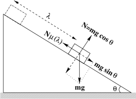
FIG. 1.: Schematic representation for the block sliding on a chute. $\lambda$ is the displacement from the initial block position. The friction force depends on the block’s position.

Because of the random character of the multicontact interface, it is on the other hand physically reasonable to assume that the coefficient of friction is not constant but changes randomly from point to point. In this case the stopping length $\lambda$ becomes a stochastic variable, and we are interested here in calculating the probability $A(\lambda)$ for the block to stop at a given position $\lambda$. We will show that under certain circumstances (e.g. close to the critical angle), fluctuations in the friction coefficient can have important observable consequences, and in particular that such fluctuations give rise to a power-law distribution of stopping distances.

For simplicity we assume $\mu(\ell)$ to be an uncorrelated random function of position, i.e.

$$\mu(\ell)\quad = \overline{\mu}-\eta(\ell)\qquad\hbox{where}$$ (3)

$$\langle\eta(\ell)\rangle = 0$$ (4)

$$\langle\eta(\ell)\eta(\ell^{\prime})\rangle = \sigma^{2}\delta(\ell-\ell^{\prime})$$ (5)

So that (2) now reads

$$\frac{\partial k(\ell)}{\partial\ell}=V+\eta(\ell)$$ (6)

where $V=\tan{\theta}-\overline{\mu}$ is the mean drift, and $\eta(\ell)$ is a noise term. If the mean drift $V$ is positive, clearly there will be a finite probability for the block never to stop. For $V<0$ on the other hand the block always stops.

This problem can be easily implemented numerically [9]. In our numerical implementation both the block and the plane surfaces are represented by finite sequences of 0s and 1s, each bit corresponding to a small region of length $a$. If a given region of the surface is “prominent”, the corresponding bit is set to one. Similarly if that region is “deep”, the corresponding bit is set to 0. Thus the profile of these surfaces is represented by strings of bits which are set to one with probability $C_{p}$ and $C_{b}$ for the plane and block respectively. One says that the block and plane are in contact at a given point whenever both the plane bit and the block bit that sits on top of it are set to one. Assuming that the friction coefficient is proportional to the number of “regions” in contact, $\mu(\ell)$ at position $\ell$ takes the value

$$\mu(\ell)=b\frac{N(\ell)}{N_{\rm max}},$$ (7)

where $N(\ell)$ is the number of microcontacts, $N_{\rm max}$ is the block length in bits and $b$ is a constant that can be associated to the contact stiffness. Equation (7) is similar to the one proposed by Bowden and Tabor [4]. The dynamic evolution dictated by equation (2) can be discretized and, after each displacement of length $a$ (one bit), the kinetic energy loss is calculated as

$$\Delta k=a\left(\tan(\theta)-\frac{bN(t)}{N_{max}}\right).$$ (8)

The block is moved on the plane in single-bit steps until the kinetic energy vanishes. The critical angle $\theta_{c}$ is defined by taking $\langle\Delta k\rangle=0$ in (8) and gives

$$\tan\theta_{c}={\overline{\mu}}=bC_{p}C_{b},$$ (9)

FIG. 2.: Distribution $A(\lambda)$ of stopping lengths as obtained numerically for the one-bit-block model. Averages were taken over $10^{8}$ realizations with an initial reduced kinetic energy $k_{0}=7.21~{}10^{-6}m$ ($v_{0}=10^{-2}m/s$ and $g=9.810m/s^{2}$) and a critical angle $\theta_{c}=45^{o}$. The inclination angle $\theta$ of the plane was: $35^{o}$ (circles), $40^{o}$ (squares), $44^{o}$ (diamonds), $44.9^{o}$ (triangles) and $44.99^{o}$ (crosses). The dashed line corresponds to $A(\lambda)=\lambda^{-3/2}$. The same exponent was found experimentally [8].

In the limit in which the average sliding is much larger than the block size in bits, (i.e. if $v_{0}$ is large, or $\theta$ is close to $\theta_{c}$) one does not expect any dependence of the results on the length $N_{\rm max}$ of the block, as long as the distribution of the friction coefficient $\mu$ has a constant mean and width. In this case it is numerically convenient to take a block length of one bit (which is always set to one). The plane bits on the other hand are set to one with probability $C_{b}$. In this case $\mu$ takes the values $0$ and $b$ with probabilities $1-C_{p}$ and $C_{p}$ respectively, so that $\overline{\mu}=bC_{b}$ . Fig. 2 shows our numerical results for this single-bit implementation. We have used $C_{p}=0.5$ and $b=2$, i.e. ${\overline{\mu}}=1$, therefore $\theta_{c}=\pi/4$. The initial reduced kinetic energy was $k_{0}=7.21~{}10^{-6}m$ ($v_{0}=10^{-2}m/s$ and $g=9.810m/s^{2}$). Averages were performed over $10^{8}$ realizations for each value of $\theta$. When $\theta\to\theta_{c}$ we find that $A(\lambda)\sim\lambda^{-3/2}$, for $\lambda$ smaller than a $\theta$-dependent cutoff $\xi(\theta)$. This behavior is in partial agreement with the experimental results of BG [8]. While the exponent they find is consistent with $3/2$, they do not report any evidence for the existence of a finite cutoff. According to our results, a very large number of experimental realizations would be needed before a cutoff can be clearly distinguished in $A(\lambda)$. As can be seen by integrating the data in Fig. 2, for deviations from the critical angle as large as $10\%$, $A(\lambda)$ only deviates from a power-law behavior for very large events, which have a small probability $10^{-5}$ to happen. This means that one needs of order $10^{5}$ realizations in order to assess the existence of a cutoff in $A(\lambda)$. Notice however that BG only performed $10^{3}$ repetitions of their measurements for each set of parameters, and this explains why only the power-law regime is observed in their experiments.

FIG. 3.: Numerical results for the mean stopping length (circles) and “cutoff length” (diamonds) as functions of $-V$. The solid line (dashed line) corresponds to $\langle\lambda\rangle\propto|V|^{-1}$ ($\xi\propto|V|^{-2}$).

Fig. 3 displays the mean stopping length $\langle\lambda\rangle$ and the “cutoff” $\xi$ versus $V\propto(\theta_{c}-\theta)$, calculated from the data in Fig. 2. When $\theta\rightarrow\theta_{c}$ ($V\to 0$) we find that $\langle\lambda\rangle\sim(\theta_{c}-\theta)^{-1}$ and $\xi\sim(\theta_{c}-\theta)^{-2}$ approximate well our numerical results. This is in slight discrepancy with BG who report that $\langle\lambda\rangle\sim(\theta_{c}-\theta)^{-0.23}$ [8].

III Mapping to a FPT problem

Since $k(\ell)$ satisfies equation (2) the problem of finding $A(\lambda)$ is readily mapped onto a First-Passage-Time (FPT) problem for a random walker with nonzero drift. The reduced kinetic energy $k(\ell)$ (which is the “position” variable $x$ of the random walker), starts at $x_{0}=k(0)=v_{0}^{2}/2g\cos{\theta}$, and executes a random walk with mean drift $V=\tan{\theta}-\overline{\mu}$. In this picture $\ell$ has the meaning of a “time” variable, and we say that the sliding-block has stopped at time $t_{\rm max}$ if its kinetic energy becomes zero at position $\lambda=t_{\rm max}$. Thus the distribution of stopping distances $A(\lambda)$ is the distribution of First-Passage-Times for a random walker to cross $x=0$. This problem turns out to be exactly equivalent to the “Gambler’s Ruin” problem [10, 11], in which one asks for the probability for a gambler with an initial capital $k_{0}$ not to have reached its ruin in $\lambda$ games if it makes an average win $V$ in each run. Fig. 4 shows a schematic representation of the equivalent FPT problem.

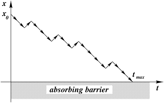
FIG. 4.: A walker starts at position $x_{0}$ at $t=0$ and executes a random walk with mean drift $V<0$. The distribution of times $t=t_{\rm max}$ for which the position becomes zero for the first time can be calculated from the probability distribution for a random walker with an absorbing barrier at $x=0$.

Equivalently one can ask for the distribution probability $W(x,t)$ for a random walker to be at position $x$ at time $t$, when there is an absorbing barrier at $x=0$. The “flux” of particles at $x=0$ gives then the desired distribution of First-Passage-Times $A(t)$. Because of these mappings, the sliding-block problem with uncorrelated random friction turns out to be completely equivalent to Compact Directed Percolation with an absorbing wall [12](CDPW - See also [13]), which is exactly solvable, and analogous to Directed Percolation with an absorbing wall (DPW) [14], which has not yet been solved analytically.

Although this classical random-walk problem has been solved in many different contexts (e.g. [10, 11, 12, 13]), an exact solution is briefly derived here for self-containedness. Let $W(x,t)$ be the probability for the block to have reduced kinetic energy $k=x$ after traversing a distance $\ell=t$. Since $k(\ell)$ satisfies the stochastic equation (2), $W(x,t)$ is a solution of the Fokker-Planck equation [15]

$$\frac{\partial W(x,t)}{\partial t}=\left(-V\frac{\partial}{\partial x}+D\frac{\partial^{2}}{\partial x^{2}}\right)W(x,t)$$ (10)

where $D=\sigma^{2}/2$. Since the particle stops, i.e., it is eliminated from the system, when its kinetic energy becomes zero, one has to solve (10) with absorbing boundary condition at $x=0$

$$W(x,t)|_{x=0}=0\qquad\hbox{for all $t$}.$$ (11)

The initial condition is $W(x,0)=\delta(x-k_{0})$ if the block starts with a well defined energy $k_{0}$. The Green function of (10) is

$$G(x,t,V,D,k_{0})=\frac{1}{\sqrt{4\pi Dt}}\exp{\left\{-\frac{(x-k_{0}-Vt)^{2}}{4Dt}\right\}}$$ (12)

in terms of which the solution of (10) plus (11) is[16]

$$W(x,t)=G(x,t,V,D,k_{0})-G(x,t,V,D,-k_{0})\quad e^{-k_{0}V/D}$$ (13)

The probability $P(t)$ for the block not to have stopped (the random walker not to have been absorbed) at time $t$ is

$$P(t)=\int_{0}^{\infty}W(x,t)dx$$ (14)

and thus the probability $A(t)$ to be absorbed at time $t$ is

$$A(t)=-\frac{\partial P(t)}{\partial t}=-\int_{0}^{\infty}\dot{W}(x,t)dx$$ (15)

Now using the fact that $W(x,t)$ satisfies the Fokker-Planck equation (10), it is readily shown that

$$A(t)=-S(x,t)|_{x=0}$$ (16)

where $S(x,t)$ is the conserved flux

$$S(x,t)=\left(V-D\frac{\partial}{\partial x}\right)W(x,t)$$ (17)

so that finally

$$A(t)=\frac{k_{0}}{\sqrt{4\pi Dt^{3}}}\exp{\left\{-\frac{(k_{0}+Vt)^{2}}{4Dt}\right\}}$$ (18)

In Fig. 5 we compare this exact solution with our numerical measurements for the single-bit model. For a RW with step length $a=1$ is readily found that $D=0.5$. We set $k_{0}=7.21~{}10^{-2}m$ ($v_{0}=1m/s$ and $g=9.810m/s^{2}$). The agreement between analytical and numerical results is very good.

FIG. 5.: Comparison of numerical and analytical results for the stopping probability $A(t)$. Averages were taken over $10^{7}$ simulations with $k_{0}=7.21~{}10^{-2}m$ ($v_{0}=1m/s$ and $g=9.810m/s^{2}$) for each chute inclination. Lines indicate the theoretical result (Equation 18) for $\theta=15^{o}$ (long-dashed line), $40^{o}$ (dotted line), $44.9^{o}$ (dashed line) and $\theta=44.99^{o}$ (dot-dashed line). For $\theta=15^{o}$ and $\theta=40^{o}$ we show the results of the simulation as small filled points. The circles are the results for $\theta=44.9^{o}$. The solid line corresponds to the behavior found in the experiments [8], $A(t)\propto t^{-3/2}$.

Fig. 6 shows $A(t)$ from equation (18) for several values of $V$ which are taken to be powers of $1/2$ for convenience. Notice that for $V<0$ the area under $A(t)$ is constant and equal to one, meaning that the block always stops. For positive $V$ on the other hand, this area is less than one, meaning that there is a finite ($V$-dependent) probability for the block never to stop, i.e. to “escape” to infinity.

Exactly at the critical angle (i.e. for $V=0$) one obtains

$$A(t)=\frac{k_{0}}{\sqrt{4\pi Dt^{3}}}\exp{\left(-\frac{k_{0}^{2}}{4Dt}\right)}$$ (19)

For large times ($Dt>>k_{0}^{2}$) this gives

$$A(t)\sim\frac{k_{0}}{\sqrt{4\pi Dt^{3}}},$$ (20)

which is consistent with our numerical measurements.

a)      b)

FIG. 6.: Stopping probability per unit time $A(t)$ for $D=0.5$, $k_{0}=7.21~{}10^{-4}m$ ($v_{0}=10{-1}m/s$ and $g=9.81~{}m/s^{2}$). The drift $V$ takes the values a) $-(1/2)^{7},-(1/2)^{6},-(1/2)^{5},...$, and b) $(1/2)^{7},(1/2)^{6},(1/2)^{5},...$. For $V=0$ one has that $A(t)\sim t^{-3/2}$.

The escape probability $\phi=P(\infty)$ is plotted in Fig. 7 as a function of $V$. This probability is small if $V$ is small, thus there is a continuous phase transition at $V_{c}=0$. As customary [12], for $V\sim 0+$ we write

$$\phi(V)\sim V^{\beta_{1}},$$ (21)

which defines the critical exponent $\beta_{1}$. For finite times, $P(t,V)=1-\int_{0}^{t}A(\tau)d\tau$ measures the probability for the particle to be “alive”. Usual scaling arguments allow one to write, for $t$ large and $|V|<<1$,

$$P(t,V)\sim t^{-\delta}f(t/\xi(V))$$ (22)

with $\xi(V)$ a correlation time diverging at $V_{c}=0$ as $\xi\sim|V|^{-\nu_{\parallel}}$, and $\delta=\beta_{1}/\nu_{\parallel}$. The scaling function $f(x)$ satisfies $f\to const.$ when $x\to 0$, thus when $V=0$ one has that $P_{t}\sim t^{-\delta}$, i.e. the power-law decay of correlations that is typical of a critical point.

FIG. 7.: Order parameter $\phi=P(\infty)=1-\int_{0}^{\infty}A(\tau)d\tau$ as function of $V$. As can be seen $\phi=0$ when $V<0$, i.e. the block always stops, which is a consequence of the drift pushing it towards the barrier (the angle being less than critical). For positive $V$ on the other hand, the drift tends to push the particle away from the barrier (the angle is larger than critical) and $\phi>0$, i.e. there is a finite probability of escape to infinity. There is a second-order phase transition at $V_{c}=0$.

Now it is easy to calculate $\beta_{1}$ and $\nu_{\parallel}$. Since $\partial P(t,V)/\partial t=-A(t)$ one has that at $V=0$ $A(t)$ behaves as $t^{-(1+\delta)}$. Therefore equation (20), implies $\delta=1/2$, in agreement with BG experimental results [8].

The “cutoff” time $\xi$ for finite but small $V$ results from the condition that the argument of the exponential in (18) be larger than one. Thus solving $(k_{0}+V\xi)^{2}=4D\xi$ one obtains $\xi\sim 2D/V^{2}$ i.e. $\nu_{\parallel}=2$. Therefore $\beta_{1}=1$. This last value can be confirmed using (21), since

$$\phi(V) = 1-\int_{0}^{\infty}A(\tau,V)d\tau=\int_{0}^{\infty}\{A(\tau,-V)-A(\tau,V)\}d\tau$$ (23)

$$= 2\sinh\left(\frac{Vk_{0}}{2D}\right)\int_{0}^{\infty}\frac{k_{0}}{\sqrt{4\pi Dt^{3}}}\exp{\left(-\frac{k_{0}^{2}+V^{2}t^{2}}{4Dt}\right)}$$ (24)

which for small $V$ gives $\phi\sim V$ since the integral gives a constant value in this limit.

The third independent exponent, and the last one needed to fully characterize the critical behavior in DP is the “meandering exponent” $\chi$ defined by $\langle x^{2}\rangle-\langle x\rangle^{2}\sim t^{\chi}$ with $\chi=2\nu_{\perp}/\nu_{\parallel}$ and $\nu_{\perp}$ associated to the divergence of “space” correlations $\xi_{\perp}\sim|V|^{-\nu_{\perp}}$. For a random walk we have $\langle x^{2}\rangle-\langle x\rangle^{2}\sim t$ and thus $\chi=1$ implying $\nu_{\perp}=1$.

From the values of these exponents one can conclude that for $V\to 0^{-}$ the mean stopping time $\langle\lambda\rangle$ behaves as $\langle\lambda\rangle\sim|V|^{-\tau_{1}}$ with [14] $\tau_{1}=\nu_{\parallel}-\beta_{1}=1$. This again is in good agreement with our numerical measurements.

IV Conclusions

This work shows that most of the experimental results obtained by Brito & Gomes for sliding blocks on a chute [8] can be reproduced by a very simple model. Compared with the traditional problem of a block sliding on a chute, a random friction coefficient is the only new ingredient in our study. The problem of finding the distribution of stopping lengths is equivalent to a first-passage-time random walk problem for an uncorrelated random walker with zero drift, and thus exact analytical solution. We derive this solution and compare its predictions with numerical results, obtaining a perfect agreement. At the critical angle $\theta_{c}=\arctan\overline{\mu}$, a power-law distribution of stopping distances is obtained: $A(\lambda)\sim\lambda^{-3/2}$ in good agreement with experimental findings. However, a discrepancy arises for the mean sliding length $\langle\lambda\rangle$, which is in this work found to behave as $\langle\lambda\rangle\sim|V|^{-1}$, while BG report $\langle\lambda\rangle\approx|V|^{-0.23}$. We believe that this difference is due to uncontrolled experimental errors, mainly because of the difficulty involved in the measurement of $\langle\mu\rangle$ (and thus $\theta_{c}$) on real systems.

REFERENCES

- [1] E-mail: arlima@if.uff.br
- [2] M.S. Vieira and H.J. Herrmann, Phys. Rev. E 49, 4534 (1994); T. Pöschell and H.J. Herrmann, Physica A 198, 441 (1993); N.A. Lindop and H.J. Jensen, Simulations of the velocity dependence of the friction force, cond-mat/9510097; Y.F. Lim and K. Chen, Phys. Rev. E 58, 5637 (1998); M. Weiss and F.-J. Elmet, Z. Phys. B 104, 55 (1997); A. Tanguy and S. Roux, Phys. Rev. B 55, 2166 (1997); A. Johanssen and D. Sornette, Phys. Rev. Lett. 82, 5152 (1999).
- [3] Friction, Arching, Contact Dynamics, D.E. Wolf and P. Grassberger (eds.), (World Scientific, Singapore, 1996) and references therein.
- [4] F.P. Bowden and D. Tabor, The Friction and Lubrication of Solids, (Clarendon Press, Oxford, 1950).
- [5] T. Baumberger and P. Berthoud, in Friction, Arching, Contact Dynamics, D.E. Wolf and P. Grassberger (eds.), (World Scientific, Singapore, 1996).
- [6] I. Webman, J.L. Gruver and S. Havlin, Physica A 266, 263 (1998).
- [7] C. Caroli and B.Velicky, in Friction, Arching, Contact Dynamics, D.E. Wolf and P. Grassberger (eds.), (World Scientific, Singapore, 1996).
- [8] V.P. Brito and M.A.F. Gomes, Phys. Lett. A 201, 38 (1995).
- [9] A.R. Lima, C. Moukarzel and T.J.P. Penna, Int. J. Mod. Phys. C 9, 875 (1998).
- [10] W. Feller, An Introduction to Probability Theory and its Applications, (Wiley, NY, 1968).
- [11] A. Papoulis, Probability, Random Variables, and, Stochastic Process, (McGraw-Hill, NY, 1965).
- [12] J.C. Lin, Phys. Rev. A 45, R3394 (1992); J.W. Essam and D. TanlaKishani, J. Phys. A: Math. Gen. 27, 3743 (1994).
- [13] E. Domany and W. Kinzel, Phys. Rev. Lett. 47, 5 (1981); F.Y. Wu and H.E. Stanley, Phys. Rev. Lett. 48, 775 (1982); E. Domany and W. Kinzel, Phys. Rev. Lett. 53, 311 (1984);
- [14] K.B. Lauritsen, K. Sneppen, M. Markosová and M.H. Jensen, Physica A 247, 1 (1997); P. Fröjdh, M. Howard and K.B. Lauritsen, J. Phys. A: Math. Gen. 31, 2311 (1998); K.B. Lauritsen, P. Fröjdh and M. Howard, 1998, Phys. Rev. Lett. to appear.
- [15] H. Risken, The Fokker-Planck equation, 2nd. Edition, (Springer 1989).
- [16] N.T.J. Bailey, The elements of Stochastic Processes with applications to the natural sciences, (Wiley publishing, 1990).