Competing frustration and dilution effects on the antiferrromagnetism in La_2-xSr_xCu_1-zZn_zO₄

Abstract

The combined effects of hole doping and magnetic dilution on a lamellar Heisenberg antiferromagnet are studied in the framework of the frustration model. Magnetic vacancies are argued to remove some of the frustrating bonds generated by the holes, thus explaining the increase in the temperature and concentration ranges exhibiting three dimensional long range order. The dependence of the Néel temperature on both hole and vacancy concentrations is derived quantitatively from earlier renormalization group calculations for the non–dilute case, and the results reproduce experimental data with no new adjustable parameters.

Since the discovery of high-$T_{c}$ superconductors much effort was invested in the investigation of the effect of dopants on the magnetic properties of the parent compounds La₂CuO₄ (LCO) and YBa₂Cu₃O₆ (YBCO). It is now well established that even a very small dopant concentration, which introduces a concentration $x$ of holes into the CuO₂ planes, strongly reduces the Néel temperature, $T_{N}$. In LCO, doped with strontium or with excess oxygen, the antiferromagnetic long range order (AFLRO) disappears at a hole concentration $x_{c}\approx 2\%$ [1], while in YBCO $x_{c}\approx 3.5\%$ [2, 3]. In contrast, the effect of Cu dilution by nonmagnetic Zn is much weaker. Like in percolation, the AFLRO persists at Zn concentration, $z$, as large as 25 % [4].

Recently, Hücker and coworkers [4] studied the phase diagram of La_2-xSr_xCu_1-zZn_zO₄, and found surprising results: It appears that the vacancies introduced by Zn doping weaken the destructive effect of holes (introduced by the Sr) on the AFLRO. E. g., in a sample with $z=15\%$, the critical concentration $x_{c}$ of the holes is approximately 3%, i.e. larger than in vacancy free LCO. Also, at $x=0.017$ the Néel temperature has a maximum as function of $z$, implying a reentrant transition! To explain these phenomena, Hücker et al. measured the variable range hopping conductivity in their samples (at temperatures lower than 150 K all samples were insulators), and showed that Zn doping lowers the localization radius of the holes. Their qualitative conclusion was that as the holes become more “mobile”, their influence on $T_{N}$ increases. However, so far there has been no quantitative understanding of the combined dependence of $T_{N}$ on both $x$ and $z$.

In this paper we present a quantitative calculation, which reproduces all the surprising features of the function $T_{N}(x,z)$. Our theory extends an earlier calculation [5], which treated the effects of quenched hole doping on the AFLRO in Sr doped LCO, i. e. calculated $T_{N}(x,0)$. The same parameters were then used to reproduce the observed $T_{N}(x)$ for the bi-layer Ca doped YBCO [6]. Here we reproduce the full function $T_{N}(x,z)$, with practically no additional adjustable parameters.

Our theory is based on the frustration model [7], which argues that when a hole is localized on a Cu–O–Cu bond [8, 9], it effectively turns the interaction between the Cu spins strongly ferromagnetic, causing a canting of the surrounding Cu moments with an angle which decays with the distance $r$ as $1/r$. The frustrating bond thus acts like a magnetic dipole [7, 10]. As argued in Ref. [5], similar dipolar effects also arise when the hole is localized over more than one bond. The frustration model also predicted a magnetic spin glass phase for $x>x_{c}$ [7], as recently confirmed in detail in doped LCO and YBCO [3, 11, 12, 13]. Furthermore, the model successfully reproduced the local field distributions observed in NQR experiments [14]. In earlier work, Glazman and Ioselevich [15] analyzed the planar non–linear $\sigma$ model with random dipolar impurities, assuming that the dipole moments are annealed and expanding in $x/T$. In Ref. [5] we generalized that analysis, treating the dipoles as quenched. The two calculations coincide to lowest order in $x$, but our renormalization group analysis allows a calculation of $T_{N}$ all the way down to zero at $x_{c}$, supplying a good interpolation between these two limits.

In what follows we summarize that theory, with emphasis on the changes necessary for including the Zn vacancies. We argue that the main effects of the vacancies enter in two related ways. First, the concentration $z$ of the Zn vacancies renormalizes the concentration of frustrated bonds; when a Cu ion is missing from (at least) one end of a “frustrated” bond, then this bond is no longer acting like a “dipole”. The probability to find a bond without vacancies on both ends is $(1-z)^{2}$, and therefore the effective concentration of “dipolar” bonds is equal to

$$y=x(1-z)^{2}.$$ (1)

Second, when one Cu ion at an end of a hole–doped bond is replaced by Zn, then the strong antiferromagnetic coupling between the spins of the second Cu and of the hole on the oxygen will form a singlet, which is equivalent to a magnetic vacancy also on the second Cu. Hence the holes increase the number of vacancies, turning their effective concentration into

$$v=z[1+2x(1-z)].$$ (2)

In what follows, we shall concentrate on the regime $x<0.03$, where the $x$-dependence of $v$ on $x$ is very weak.

Following Ref. [5], we descibe the system by the Hamiltonian

$${\cal H}={\cal H}_{v}+{\cal H}_{d},$$ (3)

where ${\cal H}_{v}$ is the non–linear sigma model (NL$\sigma$M) Hamiltonian in the renormalized classical region [16], representing the long wave length fluctuations of the unit vector ${\bf n}({\bf r})$ of antiferromagnetism. In the presence of short-range inhomogeneity, this Hamiltonian can be written as

$${\cal H}_{v}={1\over 2}\int d{\bf r}\rho_{s}({\bf r})\sum_{i,\mu}(\partial_{i}n_{\mu})^{2}.$$ (4)

Here $i=1,...,d$ and $\mu=1,...,{\cal N}$ run over the spatial Cartesian components and over the spin components, respectively, $\partial_{i}\equiv\partial/\partial x_{i}$, and the effective local stiffness $\rho_{s}({\bf r})$ is a random function. The spatial fluctuations $\delta\rho_{s}({\bf r})$ of this function are $\delta$-correlated: $[\delta\rho_{s}({\bf r})\delta\rho_{s}({\bf r^{\prime}})]=K\delta({\bf r}-{\bf r^{\prime}})$, where […] means quenched averages. Simple A power counting arguments show [5] that $K$ is irrelevant in the renormalization group sense. Therefore, we can replace $\rho_{s}({\bf r})$ in Eq. (4) by its quenched average $\rho_{s}(v)\equiv[\rho_{s}({\bf r})]$. A

${\cal H}_{d}$ is constructed [15] to reproduce the dipolar canting of the spins at long distances. Denoting by ${\bf a}({\bf r}_{\ell})$ the unit vector directed along the frustrating bond at ${\bf r}_{\ell}$, and by $M_{l}{\bf m}({\bf r}_{\ell})$ the corresponding dipole moment (where ${\bf m}({\bf r}_{\ell})$ is a unit vector giving the direction of the dipole, and $M_{l}$ is its magnitude), we have

$${\cal H}_{d}=\rho_{s}(v)\int d{\bf r}\sum_{i}{\bf f}_{i}({\bf r})\cdot\partial_{i}{\bf n},$$ (5)

with

$${\bf f}_{i}({\bf r})=\sum_{\ell}\delta({\bf r}-{\bf r}_{\ell})M_{\ell}a_{i}({\bf r}_{\ell}){\bf m}({\bf r}_{\ell}),$$ (6)

where the sum runs only over doped bonds which frustrate the surrounding (namely have both Cu ions present).

As argued in Ref. [5], the renormalization group procedure generates an effective dipole–dipole interaction between the dipole moments, $\{{\bf m}({\bf r})\}$, which is mediated via the canted Cu spins. At low temperature $T$ these moments develop very long ranged spin–glassy correlations, and may thus be considered frozen. Hence, we treat all the variables ${\bf r}_{\ell}$, ${\bf a}({\bf r}_{\ell})$, and ${\bf m}({\bf r}_{\ell})$ as quenched, and we have

$$\bigl{[}f_{i\mu}({\bf r})f_{j\nu}({\bf r}^{\prime})\bigr{]}=\lambda\delta_{\mu\nu}\delta_{ij}\delta({\bf r}-{\bf r}^{\prime}).$$ (7)

Here $\lambda=Ay$, $A=M^{2}Q/d$, where $Q=[m_{\mu}^{2}({\bf r})]$, and the effective dipole concentration $y$ replaces the parameter $x$ used in Ref. [5].

With these assumptions, we have now mapped our problem to that treated in Ref. [5]. We can thus take over the results from there, and $T_{N}(x,z)$ should be equal to the Néel temperature derived there for hole concentration $y$ and stiffness constant $\rho_{s}(v)$.

The renormalization group analysis of the Hamiltonian (3) [5] found the two–dimensional antiferromagnetic correlation length $\xi_{2D}$, as function of the two parameters $t=T/\rho_{s}$ and $\lambda$. The results contain exact exponential factors, which give the leading behavior, and approximate prefactors. For doped LCO, the results were given for two separate regimes:

$$\xi_{2D}/a=C_{1}\lambda^{0.8}\exp\Bigl{(}\frac{2\pi}{3\lambda}\Bigr{)}$$ (8)

for $t<\lambda$, and

$$\xi_{2D}/a=C_{2}\exp\Bigl{(}\frac{2\pi}{3\lambda}\bigl{[}1-\bigl{(}1-\frac{\lambda}{t}\bigr{)}^{3}\Bigr{]}\Bigr{)}$$ (9)

for $t>\lambda$. Here, $a=3.8\AA$ is the lattice constant, and the coefficients $C_{1}$ and $C_{2}$ may have a weak dependence on $t$ and on $\lambda$. In Ref. [5] the data on La_2-xSr_xCuO₄ were fully described by the constant values $C_{1}=0.74$ and $C_{2}=0.5$.

The three dimensional (3D) Néel temperature was then derived from the relation

$$\alpha\xi_{2D}^{2}\sim 1,$$ (10)

representing the appearance of 3D AFLRO due to the weak relative spin anisotropy or the weak relative interplanar exchange coupling, both contained in the parameter $\alpha$. Combining Eqs. (8) and (10) thus yields an $\alpha$-dependent value for the critical value $\lambda_{c}$, above which AFLRO is lost. This value should give the critical line for all $t<\lambda$. Using the undoped value $\alpha\sim 10^{-4}$ [1], Ref. [5] estimated $\lambda_{c}\approx 0.37$. Assuming that $\alpha$ is independent of either $y$ and $v$, this yields $y_{c}=\lambda_{c}/A\approx 0.019$, where we have used the value $A=20$ found for slightly doped LCO [5]. Combining this with Eq. (1), we thus find

$$x_{c}\approx\frac{0.019}{(1-z)^{2}},$$ (11)

showing an increase of the antiferromagnetic regime with increasing $z$. At $z=0.15$, this would predict $x_{c}\approx 0.026$, slightly lower than the observed value. This discrepancy could result from various sources. For example, dilution may affect the nearest neighbor exchange energy in the plane, $J$, more strongly than the interplanar interaction or the anisotropy. This would imply that $\alpha$ increases with $z$.

Combining Eqs. (9) and (10), one finds that for $t>\lambda$, the critical line is given by

$$\frac{t_{N}(\lambda)}{t_{N}(0)}\approx\frac{B\lambda}{1-(1-3B\lambda)^{1/3}},$$ (12)

where

$$B=-\frac{1}{4\pi}\ln(\alpha C_{2}^{2})\equiv\frac{1}{t_{N}(0)}.$$ (13)

We next look at the dependence of $T_{N}$ on $x$ for fixed $z$. Ignoring the weak dependence of $v$ on $x$ in Eq. (2), $\rho_{s}$ is assumed to depend only on $z$ (the relative error in $\rho_{s}$ from neglecting $x$ in Eq. (2) is less than 3%, see below). In that case, $\rho_{s}$ drops out of the ratio on the LHS in Eq. (12), which becomes equal to $T_{N}(x,z)/T_{N}(0,z)$. The RHS of that equation now depends only on $\lambda=Ay=Ax(1-z)^{2}$, reflecting a universality of the plot of $T_{N}(x,z)/T_{N}(0,z)$ versus the rescaled variable $y=x(1-z)^{2}$. Note that this universal plot, which should describe the Néel temperature for many values of $z$, requires no new parameters; all the parameters are known from the limit $z=0$. In fact, it is worth noting that the RHS of Eq. (12) depends only on the combination $B\lambda$, so that it should also apply to other lamellar systems with different values of $B$, resulting from different values of $\alpha$.

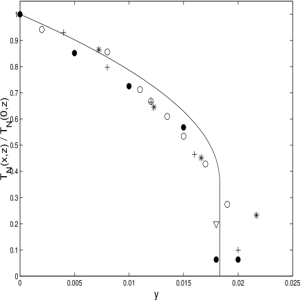
FIG. 1.: The universal plot of $T_{N}(x,z)/T_{N}(0,z)$ versus $y$, based on Eqs. (11) (for $t<\lambda$) and (12) (for $t>\lambda$). Symbols are from experiments: $z=0$: empty circles Ref. [4], full circles Ref. [19], crosses Ref. [12], triangles Ref. [3]; $z=0.15$: stars Ref. [4].

Figure 1 presents the universal plot of $T_{N}(x,z)/T_{N}(0,z)$, from both Eqs. (12) (for $t>\lambda$) and (11) (for $t<\lambda$). This theoretical curve is then compared with various experiments, for both $z=0$ and $z=0.15$. It is satisfactory to note that except for one point, the data from the latter are indistinguishable from those for the non–dilute case, confirming our universal prediction.

For comparison of the $z-$dependence of $T_{N}(x,z)$ with experiments, it is more convenient to scale $T_{N}(x,z)$ by $T_{N}(0,0)$. For that purpose, we need the ratio $T_{N}(0,z)/T_{N}(0,0)$. Theoretically, Eq. (13) yields

$$\frac{T_{N}(0,z)}{T_{N}(0,0)}=\frac{t_{N}(0,z)\rho_{s}(z)}{t_{N}(0,0)\rho_{s}(0)}=\frac{B(0)}{B(z)}\frac{\rho_{s}(z)}{\rho_{s}(0)},$$ (14)

where the weak $z-$dependence of $B(z)$ may result from such a dependence of either $\alpha$ or $C_{2}$ in Eq. (13). According to Refs. [4] and [17], the experimental data fit the linear dependence

$$\frac{T_{N}(0,z)}{T_{N}(0,0)}\approx 1-3.20z.$$ (15)

up to $z=0.25$. At low concentrations, $z<0.10$, this is in good agreement with the $1/S$ expansion result, [18] $\rho_{s}(z)/\rho_{s}(0)=1-3.14z$, if one uses the approximation $B(z)\approx B(0)$ in Eq. (14). At higher concentrations the ratio $\rho_{s}(z)/\rho_{s}(0)$ in the classical limit decreases with dilution approximately as $\rho_{s}(z)/\rho_{s}(0)=1-3.14z+1.57z^{2}$,[18] i.e. slower than the experimental $T_{N}(z)/T_{N}(0)$. This discrepancy can be due to quantum corrections to $\rho_{s}$, or to the $z$ dependence of $B$. Substituting Eqs. (14) and (15) (also replacing $z$ by $v$) into Eq. (12), we have

$${T_{N}(x,z)\over T_{N}(0,0)}=(1-3.20v){ABy\over 1-(1-3ABy)^{1/3}}.$$ (16)

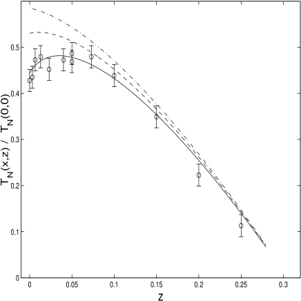
FIG. 2.: $T_{N}(x,z)/T_{N}(0,0)$ versus $z$. The full, dashed, and dash-dotted line represent Eq. (16), for $x=0.018$, $x=0.017$, and $x=0.016$ respectively. Circles are experimental data, from Ref. [4], for Sr concentration $0.017\pm 0.001$.

Figure 2 shows the dependence of $T_{N}(x,z)$ on the dilution $z$, given by the above equation, for three concentrations of holes. The theoretical curve for $x=0.018$ reproduces very well the observed maximum in the dependence of $T_{N}(x,z)/T_{N}(0,0)$ on $z$. The experimental points were measured at a nominal Sr concentration $x=0.017\pm 0.001$.

An important prediction of the theory is the high sensitivity of the maximum to the hole concentration. The maximum exists only at $x$ sufficiently close to $x_{c}$, and disappears at lower $x$. It would be interesting to check this prediction experimentally.

In conclusion, we found the combined effect of hole doping and magnetic dilution on the long-range order in lamellar Heisenberg antiferromagnets. We showed that dilution weakens the destructive effect of the holes on the AFLRO. The critical concentration $x_{c}$ increases with dilution, and the dependence of $T_{N}$ on vacancy concentration reveals a maximum, if the hole concentration is sufficiently close to $x_{c}$. These findings are in quantitative agreement with the experiment. Furthermore, the experimental data for the two concentrations agree with each other even better than with the theoretical curve, demonstrating the validity of the scaling $x\rightarrow x(1-z)^{2}$ beyond any theory. We note that the consistency of our theory with the experiments, with no new adjustable parameters, supports the validity of the frustration model.

This project has been supported by the US-Israel Binational Science Foundation. AA also acknowledges the hospitality of the ITP at UCSB, and the partial support there for the NSF under grant No. PHY94007194.

REFERENCES

- [1] e. g. B. Keimer, N. Belk, R. J. Birgeneau, A. Cassanho, C. Y. Chen, M. Greven, M. A. Kastner, A. Aharony, Y. Endoh, R. W. Erwin, and G. Shirane, Phys. Rev. B46, 14 034 (1992).
- [2] H. Casalta, H. Alloul and J.-F. Marucco, Physica C 204, 331 (1993).
- [3] Ch. Niedermayer, C. Bernhard, T. Blasius, A. Golnik, A. Moodenbaugh and J. I. Budnick, Phys. Rev. Lett. 80, 3843 (1998).
- [4] M. Hücker, V. Kataev, J. Pommer, J. Harraß, A. Hosni, C. Pflitsch, R. Gross, and B. Büchner, Phys. Rev. B59, R725 (1999).
- [5] V. Cherepanov, I. Ya. Korenblit, A. Aharony, and O. Entin-Wohlman, Eur. Phys. J. B 8, 511 (1999).
- [6] I. Ya. Korenblit, A. Aharony, and O. Entin-Wohlman, Physica B (in press).
- [7] A. Aharony, R. J. Birgeneau, A. Coniglio, M. A. Kastner, and H. E. Stanely, Phys. Rev. Lett. 60, 1330 (1988).
- [8] V. J. Emery, Phys. Rev. Lett. 58, 2794 (1987).
- [9] V. J. Emery and G. Reiter, Phys. Rev. B 38, 4547 (1988). The existence of three-spin (Cu-hole-Cu) polarons, suggested in this paper, has been confirmed recently by EPR measurements in Sr and O doped LCO [B. I. Kochelaev, J. Sichelshmidt, B. Elschner, W. Lemor, A. Loidl, Phys. Rev. Lett. 79, 4274 (1997)].
- [10] J. Villain, Z. Phys. B 33, 31 (1979).
- [11] S. Wakimoto, G. Shirane, Y. Endoh, K. Hirota, S. Ueki, K. Yamada, R. J. Birgeneau, M. A. Kastner, Y. S. Lee, P. M. Gehring and S. H. Lee, Phys. Rev. B60, R769 (1999).
- [12] J. H. Cho, F. C. Chou, and D. C. Johnston, Phys. Rev. Lett. 70, 222 (1993).
- [13] F. C. Chou, N. R. Belk, M. A. Kastner, R. J. Birgeneau, and A. Aharony, Phys. Rev. Lett. 75, 2204 (1995).
- [14] C. Goldenberg and A. Aharony, Phys. Rev. B56, 661 (1997).
- [15] L. I. Glazman and A. S. Ioselevich, Z. Phys. B 80, 133 (1990).
- [16] S. Chakravarty, B. I. Halperin, and D. R. Nelson, Phys. Rev. B39, 2344 (1989).
- [17] P. Carretta, A. Rigamonti, and R. Sala, Phys. Rev. B 55, 3734 (1997).
- [18] A. B. Harris and S. Kirkpatrick, Phys. Rev. B 16, 542 (1977).
- [19] J. Saylor and C. Hohenemser, Phys. Rev. Lett. 22, 1824 (1990).