Ferroelectric Phase Transitions in Films with Depletion Charge

Abstract

We consider ferroelectric phase transitions in both short-circuited and biased ferroelectric-semiconductor films with a space (depletion) charge which leads to some unusual behavior. It is shown that in the presence of the charge the polarization separates into ‘switchable’ and ‘non-switchable’ parts. The electric field, appearing due to the space charge, does not wash out the phase transition, which remains second order but takes place at somewhat reduced temperature. At the same time, it leads to a suppression of the ferroelectricity in a near-electrode layer. This conclusion is valid for materials with both second and first order phase transitions in pure bulk samples. Influence of the depletion charge on thermodynamic coercive field reduces mainly to the lowering of the phase transition temperature, and its effect is negligible. The depletion charge can, however, facilitate an appearance of the domain structure which would be detrimental for device performance (fatigue). We discuss some issues of conceptual character, which are generally known but were overlooked in previous works. The present results have general implications for small systems with depletion charge.

]

I Introduction

Ferroelectric perovskite materials used in memory applications usually behave as semiconductors[3]. It is expected, therefore, that at the metal-ferroelectric contact a depletion zone and the corresponding (depletion) charge distribution is formed, similar to situation with usual semiconductor-metal contacts. The corresponding electronic structure and related effects were extensively discussed for layered metal-semiconducting ferroelectric systems [4, 5, 6, 7, 8, 9, 10]. The depletion effects are especially important in switching devices [8]. The semiconducting behavior of some common ferroelectrics (PZT) was exploited in a series of papers [11, 12, 13] to account for some specific features of switching, fatigue, and rejuvenation phenomena in ferroelectric thin films.

The idea of possible importance of the depletion charge for the properties of thin ferroelectric films seems fairly natural. However, as will be shown below, ferroelectric properties in those systems are very peculiar. The consistent treatment demonstrates, in particular, that the effect of the depletion charge on thermodynamic coercive field is minute. This is a consequence of long-range Coulomb (depolarizing) field which appears simultaneously with the inhomogeneous polarization. The depolarizing field makes the problem of finding the polarization field and the point of phase transition non-local, and the local, and to a considerable extent, global dielectric response rigid. The effects of the depolarizing field were apparently neglected by the previous authors, Refs. [11, 12, 13]. Therefore, their general relevance is questionable because, as is shown below, the depolarizing field plays crucial role in determining the dielectric response and the very character of the phase transition. The depolarizing field leads to some important phenomena, like lowering of the critical temperature, $T_{c}$, possible monodomain-polydomain transition, etc.

In the present paper we describe the properties of ferroelectric films with the depletion charge in terms of the phenomenological Landau-Ginzburg-Devonshire (LGD) theory of ferroelectricity (see, e.g. [14]). We restrict ourselves to the case of a ferroelectric film with a polar axis perpendicular to the film plane. It is assumed that the charge distribution remains the same both in the paraelectric and the ferroelectric phases.

The key point in our treatment is that the polarization is divided into built-in (non-switchable) and ferroelectric (switchable) parts. Within the paper this division is mathematically strict: the built-in polarization, $P_{b}({\bf r})$, corresponds to an extremum of the LGD thermodynamic potential. The extremum corresponds to a minimum in the paraelectric and a maximum in the ferroelectric phase (the latter being similar to a zero polarization solution for a pure short-circuited crystal). We shall call the ferroelectric polarization the difference

$$P_{f}=P-P_{b}.$$ (1)

The ferroelectric polarization is switchable: there always are two equivalent solutions for $P_{f}({\bf r})$ in the ferroelectric phase. In the case of a non-zero bias we include the change of the polarization due to the bias into $P_{f},$ whereas the built-in polarization remains unchanged.

It is convenient to start with a short-circuited film of a linear dielectric with a homogeneous density of the space charge, $\rho$. The electric displacement $D$ in the film is given by the electrostatic equation div$\vec{D}=\rho,$ or simply

$$dD/dz=\rho=\text{const},$$ (2)

where $z$ is the coordinate perpendicular to the film plane. Taking into account that the voltage across the short-circuited film is zero, one finds:

$$D=(z-d/2)\rho.$$ (3)

From

$$D=\varepsilon_{0}E+P,$$ (4)

and

$$D=\varepsilon\varepsilon_{0}E,$$ (5)

one obtains for the polarization $P$:

$$P=\frac{\varepsilon-1}{\varepsilon}D.$$ (6)

Now we shall consider a ferroelectric in a paraelectric state. We shall neglect, for a moment, the nonlinearities and make some qualitative remarks. It follows from Eq. (6) that $P\approx D$ when $\varepsilon\gg 1$. Note that the electric displacement is always determined by the charge density, it does not depend on the dielectric constant [cf. (2)]. When the phase transition is approached, the dielectric constant increases, but the polarization remains practically unchanged, unlike the electric field which exhibits a strong temperature dependence. At the Curie temperature ($\varepsilon=\infty$) the field is zero in the linear approximation, while the polarization is almost the same as it was far from the transition. In other words it is more appropriate to talk about a built-in polarization rather than a built-in electric field while considering the effects of space charge in ferroelectrics. This conclusion is not limited, of course, to the case of homogeneous distribution of the space charge. For a medium with a large dielectric constant the value of the polarization is close to the value of the displacement field (6). Hence, near complete compensation of the space charge (produced by ionized donors, etc.) by the bound charges, corresponding to inhomogeneity of the polarization, occurs in a ‘soft’ dielectric medium.

The difference between the ferroelectric and non-ferroelectric (built-in) polarization can be clarified by considering effect of the bias voltage. One finds for a linear dielectric

$$D=(z-d/2)\rho+\varepsilon\varepsilon_{0}U/d,$$ (7)

where $U$ is the bias voltage and the polarization $P$ naturally splits into two parts, the switchable (‘ferroelectric’) polarization $P_{f}$ and non-switchable (‘built-in’) polarization $P_{b}$:

$$P = P_{f}+P_{b};$$ (8)

$$P_{f} \equiv (\varepsilon-1)\varepsilon_{0}U/d,$$ (9)

$$P_{b}(z) \equiv (z-d/2)\rho\frac{\varepsilon-1}{\varepsilon}.$$ (10)

Thus, in the presence of both the space charge and the bias voltage, there are two contributions to the polarization, but only one of them ‘feels’ the phase transition. The built-in polarization does not change with the bias, it remains inhomogeneous and almost insensitive to the phase transition [since $(\epsilon-1)/\epsilon\approx 1]$. The induced (ferroelectric) polarization $P_{f}=(\varepsilon-1)\varepsilon_{0}U/d\equiv$ $(\varepsilon-1)\varepsilon_{0}E_{\text{ext}}$ is homogeneous. The corresponding susceptibility $\chi_{f}\equiv dP_{f}/dE_{\text{ext}}\propto\varepsilon-1$ diverges at the transition temperature in the linear approximation. We provide more details and discussion about the division of the polarization into ferroelectric and non-ferroelectric parts below.

The paper is organized as follows. In Sec. II we analyze the problem of phase transition in a short-circuited film with homogeneous space charge. We assume that ferroelectric material is having a second-order phase transition in the bulk. We shall show that the phase transition in the film with depletion charge is inhomogeneous, with both ‘global’ and ‘local’ phase transition temperatures being lower in the film than in the bulk. Thus, the presence of the space charge will be shown to somewhat suppress the ferroelectricity.

To treat the ferroelectric phase, in Sec. III we consider a special exactly solvable case of the space charge distribution, when all the charges are located at the central plane of the film. We find that the presence of the depletion charge leads to certain lowering of the critical temperature. The corresponding lowering of the thermodynamic coercive field is shown to be minute. Therefore, the possibility of a large effect of the built-in field on switching in monodomain samples, asserted in Refs. [11, 12, 13], is rather questionable, especially since they have not considered the actual nucleation processes. Other types of the charge distribution are discussed qualitatively. In Sec. IV we show that in materials with first order phase transitions the depletion charge also effectively decreases the dielectric constant of paraelectric phase. We summarize the results in Sec. V and add there some comments of conceptual character.

II Phase transition in the presence of homogeneous space charge

A Main equations

The nonlinear electric equation of state has a usual Landau form:

$$AP+BP^{3}=E,$$ (11)

where $P(E)$ are the $z$-components of the polarization (electric field). We assume, as usual:

$$A=\alpha(T-T_{c}),\qquad B={\rm const,}$$ (12)

where $T_{c}$ is the Curie temperature and $\alpha=$const. Together with Eqs.(2),(4) and the boundary condition

$$\int_{0}^{d}Edz=U,$$ (13)

we now have the complete set of equations to treat the ferroelectric phase transition in an electroded film. Note that we cannot use Eq. (7) now because it implies a  linear relation between $D$ and $E$, whereas we are interested in a proper account for the non-linear effects.

Integrating Eq. (2), we find with the use of (4):

$$\varepsilon_{0}E(z)+P(z)=\rho z+K,$$ (14)

where $K$ is a constant which should be found from Eq. (13). We obtain:

$$\varepsilon_{0}E(z)=-P(z)+(z-d/2)\rho+\frac{1}{d}\int_{0}^{d}P(z)dz+\varepsilon_{0}E_{\text{ext}},$$ (15)

where the external field is produced by external bias voltage,

$\displaystyle E_{\text{ext}}=U/d.$

Combining this with Eq. (11) we get:

$$(A+\varepsilon_{0}^{-1})P+BP^{3}-\frac{1}{d\varepsilon_{0}}\int_{0}^{d}P(z)dz$$ (16)

$$= (z-d/2)\rho/\varepsilon_{0}+E_{\text{ext}}.$$ (17)

From Eqs. (16),(1) we obtain, up to terms $\propto P_{b}^{2}:$

$$(A+3BP_{b}^{2}+\varepsilon_{0}^{-1})P_{f}+3BP_{b}P_{f}^{2}+BP_{f}^{3}$$ (18)

$$-\frac{1}{d\varepsilon_{0}}\int_{o}^{d}P_{f}(z)dz=E_{\text{ext}}.$$ (19)

B Paraelectric phase

Let us first calculate $P_{f}$ in the paraelectric phase to the linear approximation, i.e. for small $U$. We have to solve the simple integral equation

$$(A+3BP_{b}^{2}+\varepsilon_{0}^{-1})P_{f}-\frac{1}{d\varepsilon_{0}}\int_{o}^{d}P_{f}(z)dz=E_{\text{ext}},$$ (20)

assuming that $A$ is positive. Introducing a notation

$$I\equiv\frac{1}{d\varepsilon_{0}}\int_{o}^{d}P_{f}(z)dz,$$ (21)

we find from (20):

$$P_{f}=\frac{E_{\text{ext}}+I}{A+3BP_{b}^{2}+\varepsilon_{0}^{-1}}.$$ (22)

To find $I$ we substitute this expression into Eq. (21) and, as a result, find $P_{f}$ in an explicit form:

$$P_{f}(z)=E_{\text{ext}}\frac{1}{1-G}\frac{1}{A+3BP_{b}^{2}\left(z\right)+\varepsilon_{0}^{-1}},$$ (23)

where

$$G\equiv\frac{1}{d\varepsilon_{0}}\int_{o}^{d}\frac{dz}{A+3BP_{b}^{2}+\varepsilon_{0}^{-1}}.$$ (24)

Thus:

$$1-G=\frac{1}{d\varepsilon_{0}}\int_{o}^{d}\frac{A+3BP_{b}^{2}}{A+3BP_{b}^{2}+\varepsilon_{0}^{-1}}dz\approx A+3B\langle P_{b}^{2}\rangle,$$ (25)

where $\langle\dots\rangle\equiv d^{-1}\int_{0}^{d}dz\ldots,$ and we have taken into account that typically $\varepsilon_{0}^{-1}\gg(A,3BP_{b}^{2})$.

We see, therefore, that the susceptibility $\chi_{f}=dP_{f}/dE_{\text{ext}}\propto\left(1-G\right)^{-1}$ diverges at the temperature $\tilde{T}_{c},$ which is lower that the Curie-Weiss temperature $T_{c}$ in pure crystal (Fig. 1), and the divergence of the dielectric response would take place when $A=-3B\langle P_{b}^{2}\rangle$, i.e. at $T=\widetilde{T_{c}}:$

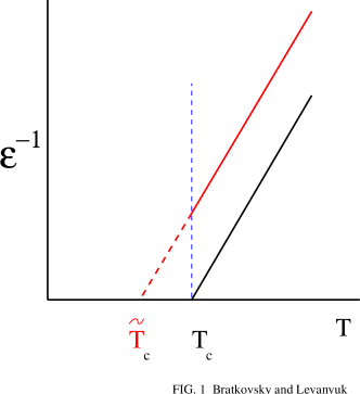
FIG. 1.: Schematic of the dielectric constant in a pure ferroelectric film and the film with uniform depletion charge (broken line). Depletion charge suppresses the critical temperature from $T_{c}$ in pure sample down to $\tilde{T}_{c}$ by $(1-100)$K (see text).

$$T_{c}-\widetilde{T_{c}}=\frac{3B\langle P_{b}^{2}\rangle}{\alpha}.$$ (26)

Let us estimate this difference. For a displacive transition $B$ and $\alpha$ have normal ‘atomic’ values[14]. For $P_{b}\approx P_{{\rm at}}$, where $P_{{\rm at}}$ is the atomic polarization, $T_{c}-\widetilde{T_{c}}$ would be about $T_{{\rm at}}\sim 10^{4}-10^{5}$K. For the charged impurity concentration $N_{d}$ one estimates $P_{b}\sim(N_{d}/N_{{\rm at}})(d/d_{{\rm at}})P_{{\rm at}}$ where $N_{{\rm at}}$ is the ‘atomic’ concentration (10${}^{22}-10^{23})$cm^-3, $d_{{\rm at}}$ is the ‘atomic’ distance (unit cell length, 3-5$\AA)$ With the donor concentration $N_{d}=10^{18}$cm^-3 [11], the thickness of the totally depleted film (equal the width of the depletion layer) would be about 2$\cdot 10^{3}\AA$, and we estimate $P_{b}\sim(10^{-2}-10^{-3})P_{{\rm at}}$ and $T_{c}-\widetilde{T_{c}}\sim(1-100)$K. We see that the phase transition temperature can be reduced substantially, i.e. the paraelectric phase can be considerably ‘harder’ than the same phase in the pure crystal.

We see already that there is a radical difference between the effects of  external field (the bias voltage) and the built-in field (polarization) on the ferroelectric transition. The former would smear out the phase transition and shift the maximum of the dielectric response to higher temperatures, while the built-in field does not lead to the maximum in the dielectric response at $A>0.$

C Ferroelectric phase

But what happens at $A<0$? This is not so easy to determine. We shall try to answer this question, at least semi-quantitatively, but first we have to explain what the difficulty is. It is seen from Eq. (23) that $P_{f}$ is inhomogeneous over the sample, being smaller near the electrodes. It is worth mentioning that inhomogeneity of $P_{f}$ under the bias voltage is different from the inhomogeneity of  the dielectric susceptibility of the paraelectric phase. Indeed, the ‘local’ dielectric susceptibility is what one would find by cutting out a small piece of the ferroelectric at a given position in the sample, making a capacitor out of this piece, and measuring its dielectric response. In our case we have to ‘fill up’ the capacitor with a medium with a given local values of $P_{b}$: i.e. it is the built-in polarization that makes the ferroelectric response of the film effectively inhomogeneous. If $P_{b}$ were constant, the Eq. (20) would have had a homogeneous solution:

$$(A+3BP_{b}^{2})P_{f}=E_{\text{ext}}.$$ (27)

One can see that the local susceptibility $\chi_{loc}(z)\equiv dP_{f}/dE_{ext}=\left(A+3BP_{b}^{2}\right)^{-1}$ is more inhomogeneous than the polarization Eq. (23): one has to compare $3BP_{b}^{2}(z)$ in the case of $\chi_{loc}$, where $A$ is small, with $A+\varepsilon_{0}^{-1}$ $\approx$ $\varepsilon_{0}^{-1}>>A$ in the latter case. The smaller inhomogeneity of the polarization $P_{f}$ in relatively more inhomogeneous dielectric medium $\left(\chi_{loc}\right)$ is due to the mutual Coulomb interaction of the bound charges (‘longitudinal’ inhomogeneity of the polarization). Consequently, the system tries to lower this energy by reducing the inhomogeneity.Therefore, the phase transition takes place in a fairly strongly inhomogeneous medium.  There is also another inhomogeneity, which is described by the second term on the left hand side of the Eq. (19). It is expected to be important in the ferroelectric phase.

In the center of the film, where $P_{b}=0$, the local susceptibility is the same as in pure crystal but at other points of the crystal it is ‘harder’ (meaning that $\chi_{loc}$ is lower), the hardest region being close to the electrodes (Fig. 2). If not for long-range Coulomb interactions, this would means that the ferroelectric phase transition would occur at the critical temperature for pure sample, $T_{c}$. However, the Coulomb interaction suppresses the phase transition across the system, ans $T_{c}$ reduces down to $\tilde{T}_{c},$ Fig. 1.

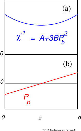
FIG. 2.: Schematic of the dielectric response $\chi_{f}^{-1}=dE_{\rm ext}/dP$ which becomes inhomogeneous in the presence of the depletion charge (a), and the built-in polarization $P_{b}$ (b).

Since the problem of the film with depletion charge proves to be fairly complicated, it is instructive to consider first some special cases, where the treatment is easier, and get a feel of the relevant effects. The most natural way to simplify the problem is to replace the continuous distribution of the built-in polarization by a stepwise distribution. The simplest problem of that type would be a charge located at a plane in the middle of the film with a constant charge density $\sigma$, Fig. 3. In this case the built-in polarization has opposite signs but the same absolute value in the two halves of the film, so that the film is homogeneously ‘hard’. It is not completely homogeneous though, there is the inhomogeneity due to the second term on the left hand side of Eq. (19). But now we can study the effects of two inhomogeneities separately, beginning with the case of a ‘harmonic’ homogeneity and a weaker ‘anharmonic’ inhomogeneity. We would expect that in this case the phase transition occurs into a monodomain state and show below that this is a justifiable assumption.

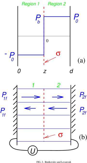
FIG. 3.: (a) Schematic of the exactly solvable case when the charge (with surface density $\sigma$) is located on a plane in the middle of a ferroelectric film under bias voltage $U$. The built-in polarization $P_{b}$ takes the values $-(+)P_{0}$, where $P_{0}=\sigma/2$, in the left (right) halves of the film (regions 1 and 2, respectively). (b) Possible domain structure with ferroelectric (switchable) polarization which has different magnitude in the left and right halves of the film.

III Phase transition in the film with special forms of the space charge distribution

A Charge located at the central plane and its effect on the coercive field

We denote by $P_{1}$, $E_{1}$ and $P_{2}$, $E_{2}$ the polarization and the field in the two halves of the short-circuited film with the external bias voltage $U$ (Fig. 3). We then have:

$$E_{1}+E_{2}=\frac{2U}{d}\equiv 2E_{\text{ext}},$$ (28)

$$\varepsilon_{0}E_{2}+P_{2}-\varepsilon_{0}E_{1}-P_{1}=\sigma,$$ (29)

$$AP_{1\left(2\right)}+BP_{1\left(2\right)}^{3}=E_{1\left(2\right)}.$$ (30)

Finding $E_{1}$, $E_{2}$ from the first two equations, one can present Eq. (30) in the form:

$$\left(A+\frac{1}{2\varepsilon_{0}}\right)P_{1}+BP_{1}^{3}-\frac{P_{2}}{2\varepsilon_{0}}=E_{\text{ext}}-\frac{\sigma}{2\varepsilon_{0}},$$ (31)

$$\left(A+\frac{1}{2\varepsilon_{0}}\right)P_{2}+BP_{2}^{3}-\frac{P_{1}}{2\varepsilon_{0}}=E_{\text{ext}}+\frac{\sigma}{2\varepsilon_{0}}.$$ (32)

By summing up these two equations we get:

$$(P_{1}+P_{2})\left[A+B(P_{1}^{2}-P_{1}P_{2}+P_{2}^{2})\right]=2E_{\text{ext}}.$$ (33)

Obviously, for the case of unbiased sample ($E_{{\rm ext}}=U=0$) there is always a solution $P_{1}=-P_{2}\equiv-P_{0}$ (Fig. 3) where $P_{0}$ is given by

$$(A+\varepsilon_{0}^{-1})P_{0}+BP_{0}^{3}=\sigma/2\varepsilon_{0}.$$ (34)

Since $P_{0}$ is much smaller than the saturation polarization $P_{s}$, and accounting for the fact that in ferroelectrics $|A|\ll\varepsilon_{0}^{-1}$ (it reads as $|A|\ll 4\pi$ in CGS units) the solution is

$$P_{0}=\sigma/2.$$ (35)

Indeed, the estimate for a typical PZT film (see below) gives $P_{0}=2.5\mu$Ccm^-2, whereas the saturation polarization $P_{s}=40\mu$Ccm^-2. We shall consider this solution as the built-in polarization and present the other solutions in the form:

$$P_{1\left(2\right)}=-(+)P_{0}+P_{1\left(2\right)f},$$ (36)

where $P_{1(2)f}$ is the ‘ferroelectric’ polarization. From Eqs. (31),(32) we have:

$$\left(A+3BP_{0}^{2}+\frac{1}{2\varepsilon_{0}}\right)P_{1f}$$ (37)

$$- \frac{P_{2f}}{2\varepsilon_{0}}-3BP_{0}P_{1f}^{2}+BP_{1f}^{3}=E_{\text{ext}},$$ (39)

$$\left(A+3BP_{0}^{2}+\frac{1}{2\varepsilon_{0}}\right)P_{2f}$$

$$- \frac{P_{1f}}{2\varepsilon_{0}}+3BP_{0}P_{2f}^{2}+BP_{2f}^{3}=E_{\text{ext}}.$$ (40)

These equations can be considered as obtained by minimization of the thermodynamic potential:

$$F = \frac{1}{2}(\widetilde{A}+\frac{1}{2\varepsilon_{0}})(P_{1f}^{2}+P_{2f}^{2})-\frac{P_{1f}P_{2f}}{2\varepsilon_{0}}$$ (43)

$$-BP_{0}\left(P_{1f}^{3}-P_{2f}^{3}\right)+\frac{B}{4}(P_{1f}^{4}+P_{2f}^{4})$$

$$-E_{\text{ext}}\left(P_{1f}+P_{2f}\right),$$

where we have introduced

$$\widetilde{A}=A+3BP_{0}^{2}.$$ (44)

It is instructive to go over to new variables, the average switchable polarization and the difference between the switchable polarizations in both halves of the film:

$$\bar{P}\equiv\frac{P_{1f}+P_{2f}}{2},\qquad\Delta P\equiv P_{1f}-P_{2f}.$$ (45)

In these variables the thermodynamic potential takes the form:

$$F = \widetilde{A}\bar{P}^{2}+\frac{B}{2}\bar{P}^{4}-2E_{\text{ext}}\bar{P}$$ (48)

$$+\frac{\widetilde{A}+\varepsilon_{0}^{-1}}{4}\Delta P^{2}-3BP_{0}\bar{P}^{2}\Delta P$$

$$-\frac{1}{2^{5/2}}BP_{0}\Delta P^{3}+\frac{B}{32}\Delta P^{4}+\frac{3}{4}B\bar{P}^{2}\Delta P^{2}.$$

The stability of the paraelectric phase ($P_{1f}=P_{2f}=0)$ will be lost at $\widetilde{A}\equiv A+3BP_{0}^{2}=0$, therefore, the parameter $\bar{P}$ is ‘critical’ at the phase transition while $\Delta P$ is ‘non-critical’, since the coefficient before $\Delta P^{2}$ does not go to zero. Now it is evident that the phase transition we discuss is second order, since there is no cubic term in $\bar{P}$. The external bias voltage couples only to $\bar{P}$, so that the phase transition for the order parameter $\bar{P}$ will be smeared out by external field, whereas it has no effect on the built-in polarization $P_{0}$. This highlights the qualitatively different response of the system to external and built-in field due to space charge.

We see from the third and fourth terms in $F$ (48) that the equilibrium value of $\Delta P$ is proportional to $\bar{P}^{2}$ and, therefore, the last three terms in (48) would implicitly contain terms higher order in $\bar{P}$, like $\bar{P}^{6}$. This would be inconsistent with the form of the Landau functional that we used initially. Therefore, the last three terms in (48) should be omitted.

Now we are in a position to find the ferroelectric polarization in the ferroelectric phase. The equilibrium values $\bar{P}$, $\Delta P$ at $\widetilde{A}<0$ are:

$$\bar{P}^{2} \equiv P_{s}^{2}=-\frac{\widetilde{A}}{B},$$ (49)

$$\Delta P = 6\varepsilon_{0}BP_{0}\bar{P}^{2}=-6\varepsilon_{0}\widetilde{A}P_{0}.$$ (50)

These formulas are approximate: we have neglected an inessential renormalization of the coefficient $B$ due to the coupling given by the fifth term on the right hand side in Eq. (48), and we have taken into account that $\mid\widetilde{A}\mid<<\varepsilon_{0}^{-1}$. Then the solution for spontaneous ferroelectric polarization is:

$$\bar{P}_{1f} = \pm\sqrt{\frac{|\widetilde{A}|}{B}}+3\varepsilon_{0}|\widetilde{A}|P_{0}=\pm P_{s}+\frac{3}{2}\varepsilon_{0}|\widetilde{A}|\sigma,$$ (51)

$$\bar{P}_{2f} = \pm\sqrt{\frac{|\widetilde{A}|}{B}}-3\varepsilon_{0}|\widetilde{A}|P_{0}=\pm P_{s}-\frac{3}{2}\varepsilon_{0}|\widetilde{A}|\sigma,$$ (52)

where +(-) sign corresponds to right- (left-) ward directed polarization in the domains, Fig. 3(b). We see that in the half of the film where the ferroelectric polarization has the same direction as the built-in polarization (right half in Fig. 3), its value, $P_{2f},$ is smaller than in another half.

B The effect of the depletion charge on a coercive field

Now we are able to estimate the effect of the depletion charge on a coercive field, and it happens to be very small. From the free energy (48) we see that the dependence of the average switchable polarization $\bar{P}$ on $E_{\text{ext}}$ has a form of a hysteresis loop

$$\widetilde{A}\bar{P}+\widetilde{B}\bar{P}^{3}=E_{\text{ext}}.$$ (53)

Here we accounted for the fact that the fifth term in the free energy (48) is actually $\propto\bar{P}^{4}$ because of (50), and this is equivalent to the renormalization of the coefficient $B\rightarrow\widetilde{B}\equiv B(1-18\varepsilon_{0}BP_{0}^{2})$.

The ‘thermodynamic’ coercive field for the hysteresis loop $\bar{P}=\bar{P}(E_{\text{ext}})$ is

$$E_{c}=\frac{2\left(-\widetilde{A}\right)^{3/2}}{3^{3/2}\widetilde{B}^{1/2}}.$$ (54)

One can easily find the hysteresis loops for $P_{1f}$ and $P_{2f}$ from Eqs. (45),(50):

$$P_{1f} = \bar{P}(E_{{\rm ext}})+3\varepsilon_{0}BP_{0}\bar{P}^{2}(E_{{\rm ext}})$$ (55)

$$P_{2f} = \bar{P}(E_{{\rm ext}})-3\varepsilon_{0}BP_{0}\bar{P}^{2}(E_{{\rm ext}})$$ (56)

The hysteresis loops are interesting since the thermodynamic coercive field is exactly the same in both halves of the film, Fig. 4, in spite of that difference in absolute values of the polarizations.

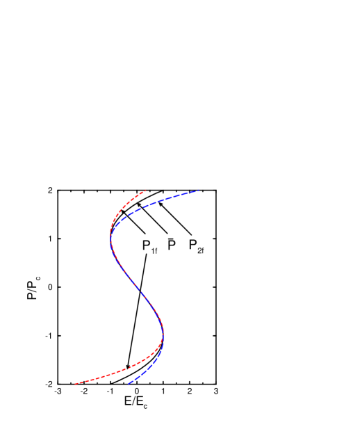
FIG. 4.: Schematic of the hysteresis loop $P=P(E_{\rm ext})$ of the film with the charge at the central plane, Fig. 3. Note that the thermodynamic coercive field $E_{c}$ is exactly the same in both halves of the film (as seen from the hysteresis loops for $P_{1f}$ and $P_{2f}$). The polarization is normalized to $P_{c}=P(E_{c})$.

Since in the ferroelectric film with depletion charge $|\widetilde{A}|<|A|,$ the coercive field there is smaller than the one, $E_{c0}$, in a sample without the space charge. The physical reason for this reduction is the lowering of the transition temperature at the phase transition point, where the coercive field is zero. Thus, one can expect that the switching would be somewhat easier in the material with the depletion charge in comparison with a pure material. This observation is only suggestive since the actual switching occurs at much lower fields and proceeds by nucleation and growth processes, whereas the ‘thermodynamic’ coercive field $E_{c}$ refers to thermodynamic limits of stability of the homogeneous polarization in the external field.

Let us estimate the change in the coercive field for typical thin PZT film not very close to the transition, $|A|\gg 3BP_{0}^{2}$, from (54)

$$E_{c}=E_{c0}-\Delta E_{c},$$ (57)

where

$$E_{c0} = \frac{2|A|^{3/2}}{3^{3/2}B^{1/2}},$$ (58)

$$\Delta E_{c} = -\frac{9}{2}E_{c0}{\frac{P_{0}^{2}}{P_{s}^{2}}}(1-2\varepsilon_{0}|A|)\approx-\frac{9}{2}E_{c0}{\frac{P_{0}^{2}}{P_{s}^{2}}},$$ (59)

where $E_{c0}$ is the coercive field in the pure material, and we again used the fact that $|A|\varepsilon_{0}\ll 1$. We now consider the PZT film of the thickness $L=300$ nm, the saturation polarization $P_{s}=40$ $\mu$C/cm², and the donor concentration $N_{d}=10^{18}$cm^-3, discussed previously [11]. With these parameters $\sigma=N_{d}L=5\mu$C/cm², $P_{0}=\sigma/2=2.5\mu$C/cm². We then find from (59)

$\displaystyle\frac{\Delta E_{c}}{E_{c}}=\frac{9}{2}\left(\frac{P_{0}}{P_{s}}\right)^{2}=\frac{9}{8}\left(\frac{\sigma}{P_{s}}\right)^{2}=0.02$

Obviously, the effect quickly gets even smaller for thinner films of practical interest, $\Delta E_{c}\propto\sigma^{2}\propto L^{2}$.

Thus, we see that the effect of the depletion charge on the coercive field exists, but it is negligible. It has been speculated that the ’experimental’ coercive field for nucleation $E_{cn}$ should be reduced by exactly the value of the built-in field $E_{b}$, $E_{cn}=E_{{\rm ext}}+E_{b}$ [11, 12, 13]. Since these authors have estimated $E_{b}\approx 100$kV/cm, whereas the observed coercive field was $E_{c}\approx 80$kV/cm[11], one would conclude that the coercive field has been suppressed by more than a half by the built-in field. However, this result and the whole previous analysis are rather questionable, since no actual nucleation processes have been considered in Refs. [11, 12, 13].

C On the possible domain structure

One sees from Eq. (51) that there is a discontinuity of the ferroelectric polarization at the central plane. It creates depolarizing field, which can, in principle, be reduced by formation of a domain structure [Fig. 3(b)]. To see if it really takes place we have to use the LGD thermodynamic potential with the energy of the electric field included explicitly:

$$F_{LGD}=\int dV\left[\frac{A}{2}P^{2}+\frac{B}{4}P^{4}+\frac{\kappa}{2}\left(\frac{dP}{dx}\right)^{2}+\frac{\varepsilon_{0}E^{2}}{2}\right],$$ (60)

where the gradient term is added because we would like to consider a possibility of domain structure formation with the domain walls perpendicular to $x$ direction, and this term gives rise to a surface energy of the walls. Once more we divide the polarization into two parts as in Eq. (1) and write

$$E=E_{b}+E_{f},$$ (61)

with obvious notations. Then

$$F_{LGD}=F_{1}+F_{2}+F_{3},$$ (62)

where

$$F_{1} = \int dV\Biggl{[}\frac{A+3BP_{b}^{2}}{2}P_{f}^{2}+BP_{b}P_{f}^{3}+\frac{B}{4}P_{f}^{4}$$ (64)

$$+\frac{\kappa}{2}\left(\frac{dP_{f}}{dx}\right)^{2}+\frac{\varepsilon_{0}E_{f}^{2}}{2}\Biggr{]},$$

$$F_{2} = \int dV\left(AP_{b}P_{f}+BP_{b}^{3}P_{f}+\varepsilon_{0}E_{b}E_{f}\right)$$ (65)

$$= \int dV\left(E_{b}P_{f}+\varepsilon_{0}E_{b}E_{f}\right)=\int dVE_{b}D_{f},$$ (66)

$$F_{3}=F_{3}(P_{b},E_{b}).$$ (67)

The energy $F_{2}=0$ for the problem of calculating the energy of the domain structure periodic along the $x$ axis, and we can consider $F_{1}$ only. The domain structure is shown in Fig. 3. We suppose that the domain width is $a<d$, otherwise the domain structure would not form. The electric field is created by the bound charges at the central plane of the film. This field is approximately

$$\frac{1}{2\varepsilon_{0}}(\bar{P}_{1f}-\bar{P}_{2f})=\frac{3\widetilde{A}}{2}P_{0},$$ (68)

and it is concentrated in a layer of width $\approx a$. The energy of this field per unit area and unit length along $x$ direction is

$$\varepsilon_{0}\widetilde{A}^{2}P_{0}^{2}a,$$ (69)

where we have omitted a numerical factor. The surface energy of the domain walls for the same region is

$$\frac{\gamma d}{a},$$ (70)

where $\gamma$ is the surface energy of the domain wall. It is known to be [14]

$$\gamma\approx\frac{\widetilde{A}^{2}}{B}\xi,$$ (71)

where $\xi$ is the domain wall width. Minimizing the total energy, one finds the period of the suspected domain structure:

$$a\sim\left(d\xi\frac{\varepsilon_{0}^{-1}}{BP_{0}^{2}}\right)^{1/2}.$$ (72)

The condition $a<d$ is fulfilled if

$$d>\frac{\varepsilon_{0}^{-1}}{BP_{0}^{2}}\xi\sim\frac{P_{{\rm at}}^{2}}{P_{0}^{2}}\xi\sim(10^{4}-10^{6})\xi.$$ (73)

We have already mentioned that $P_{{\rm at}}/P_{0}\sim 10^{2}-10^{3}$, so that the prefactor of $\xi$ is about $10^{4}-10^{6}$. Taking into account that $\xi$ is no less than the unit cell length, and that it can easily be an order of magnitude larger than that, it seems doubtful that the formation of the domain structure due to discontinuity of the polarization in the center of the film would be possible in films with $d\lesssim 10^{3}d_{{\rm at}}$. In any case, if it forms, then at fairly low temperatures, so that our initial assumption that the phase transition takes place into a monodomain state is justified. We see that the ‘anharmonic’ inhomogeneity is not the most important reason for the domain structure formation, and we shall neglect it in the future.

D Charge located at two symmetric planes

A stepwise distribution of the built-in polarization, which is more like that in Fig. 2, can be obtained with two similar symmetrically positioned charged planes (Fig. 5). We have now two ‘hard’ near electrode regions and the central ‘soft’ one. For $A+3BP_{0}^{2}>0$ the system resembles a plate of a pure ferroelectric with two ‘passive’ layers close to the electrodes. Phase transitions in a similar system (ferroelectric plate with vacuum gaps near the electrodes) were studied by Chensky and Tarasenko[15]. They found that there are transitions to both monodomain and polydomain states depending on geometrical parameters. Generalizing their consideration to the case of two dielectric layers we found that the transition to the monodomain state takes place if

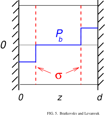
FIG. 5.: Schematic of a ferroelectric film with two charged planes inside. The charged planes lead to piece-wise built-in polarization $P_{b}$.

$$d_{1}<d_{1c}=\varepsilon_{1}\left(\frac{12\varepsilon_{0}\kappa}{\varepsilon_{\perp}}\right)^{1/2},$$ (74)

where $d_{1}$, $\varepsilon_{1}$ are the width and the dielectric constant of the ‘passive’ layer, $\varepsilon_{\perp}$ is the dielectric constant in the plane of the film (perpendicular to easy axis). In our case the value of $d_{1c}\sim d$ can be estimated as:

$$d_{1}\sim\frac{P_{{\rm at}}^{2}}{P_{0}^{2}}d_{{\rm at}}\sim(10^{4}-10^{6})\mathop{\rm\AA}.$$ (75)

This estimate is certainly crude but it seems likely that the phase transition in completely depleted films proceeds into a monodomain state. We have recently discussed a domain structure in a ferroelectric plate with ‘passive’ layers[16]. It was found that far from the phase transition a domain structure exists for however thin passive layer. Therefore, one can expect that a domain structure forms at some temperature below the phase transition in a short-circuited completely depleted ferroelectric film, but this question should to be studied in greater detail.

IV First order phase transition

It might be tempting to conclude, based on Eq. (26), that while the built-in polarization ‘hardens’ ferroelectrics with second order transition it ‘softens’ those with first order transitions, since the coefficient at $P^{4}$ in the LGD thermodynamic potential is negative in the latter case ($B<0$). However, such a hastily conclusion is almost certainly wrong.

The fact of the matter is that, while considering relatively ‘weak’ first order phase transition (otherwise the LGD theory is not applicable), one has to take into account explicitly the interaction of the order parameter with elastic deformations. Specific features of the elasticity in solids make the above statement about the sign of the coefficient $B$ before $P^{4}$ fairly vague. There are several different $P^{4}$ coefficients and some of them remain positive for weakly first order transitions[17]. To treat the problem, one has to start with the LGD potential in the form:

$$F = \frac{A}{2}P^{2}+\frac{B}{4}P^{4}+\frac{C}{6}P^{6}$$ (77)

$$+rP^{2}u_{ll}+\frac{K}{2}u_{ll}^{2}+\mu\left(u_{ik}-\frac{1}{3}\delta_{ik}u_{ll}\right)^{2},$$

where $u_{ik}$ is the strain tensor, $r$ is the electrostriction constant, $K$, $\mu$ are the bulk and the shear moduli. For a bulk sample the phase transition takes place usually in a free crystal and after minimization over the strain components one obtains:

$$F=\frac{A}{2}P^{2}+\frac{\widetilde{B}}{4}P^{4}+\frac{C}{6}P^{6},$$ (78)

where

$$\widetilde{B}=B-\frac{2r^{2}}{K}.$$ (79)

The first order of the phase transition means $\widetilde{B}<0,$ but the coefficient $B$ itself may be positive and it is indeed positive and large for not too ‘strong’ first order structural transitions, because $2r^{2}/K$ is of ‘atomic’ value in this case, and $\widetilde{B}$ is rather small.

But for a phase transition in an inhomogeneous system the above procedure does not work. One cannot minimize over the strain components because they are not independent there[18]. For our case, one can assume that all the displacements are perpendicular to the film plane so that the only relevant component of the strain tensor is $u_{zz}$. Putting all other strain components in Eq. (77) to zero and minimizing over $u_{zz}$ we obtain:

$$F=\frac{A}{2}P^{2}+\frac{\widehat{B}}{4}P^{4}+\frac{C}{6}P^{6},$$ (80)

where

$$\widehat{B}=B-\frac{2r^{2}}{K+\frac{4}{3}\mu}=\widetilde{B}+\frac{2r^{2}}{K}\frac{\frac{4}{3}\mu}{K+\frac{4}{3}\mu}.$$ (81)

It is worth mentioning that $K+\frac{4}{3}\mu$ is the modulus with respect to uniaxial extension without changing the lateral size[19]. The last factor in Eq. (81) is usually of the order of unity and if $\mid B\mid$ is not very large then $\widehat{B}>0$ and the results of Sec. II are applicable for the case considered there as well.

One might conclude that, because $\widehat{B}>0$, the first order phase transition in a bulk sample becomes second order in the film. Such a possibility is not excluded but several reservations are in order. Firstly, we have assumed that only one component of the strain tensor operates. It is a natural assumption for an infinite film but the real films are not infinite. Secondly, even for an infinite film there are various possibilities for the phase transition: it could, for instance, transform into a mixture of homogeneous and inhomogeneous (two phase) state. Which of these possibilities is realized in practice depends on the conditions that we have not specified here, e.g. on the elastic properties of the substrate. The nature of first order phase transitions in films is worth studying together with taking into account the actual experimental conditions.

In conclusion of this Section we would simply note that in materials with first order ferroelectric transition the paraelectric phase in thin depleted films becomes more ‘ferroelectrically rigid’, its dielectric constant decreases, in analogy with ferroelectrics with second order phase transition.

V Comments

We have found that the polarization in the present problem naturally separates into ‘switchable’ and ‘non-switchable’ parts in the presence of the built-in (space) charge. Obviously, only the switchable polarization may be used as an order parameter in the problem. In our example of a system with all the charge placed at the central plane the order parameter was $P-P_{0}(\vec{r})$ averaged over the sample, where $P_{0}(\vec{r})$ is the non-switchable part of the polarization. The case of a homogeneous charge in the ferroelectric proved to be too complicated and its consideration was omitted. What is the problem with selecting the order parameter in the present situation? We would like to clarify the question in this section.

One difficulty with selecting the order parameter in systems with depletion charge is that  these systems are inhomogeneous with respect to the phase transition, even when the depletion charge is homogeneous. The order parameter for a phase transition in the inhomogeneous medium is the amplitude of a function that has a space distribution of the quantity that plays a role of the order parameter in homogeneous medium. The function gives the form of the ‘most rapidly growing fluctuation’ or of the symmetry perturbation responsible for the loss of stability of a symmetric phase.

Another difficulty stems from the polarization being an electric quantity, intimately related to a distribution of the electric charge in a crystal. In defining the order parameter one has to recall that in theory the notions of the ‘order parameter’, ‘phase transition’, and so forth, implicitly refer to an infinite medium. It is ambiguous, or even meaningless, however, to consider the polarization of an infinite medium (see e.g. Ashcroft and Mermin’s book, Ch. 27). This is because the electric field in a sample is determined by the boundary conditions (shape of the sample, presence or absence of electrodes, bias voltage, etc.). One can avoid specifying the boundary conditions and still remain within rigorous definitions by considering the plane waves ${\bf P}_{k}$ of the order parameter in an infinite medium and then taking a long wave length limit ${\bf k}\rightarrow 0$. Those waves which stiffness constant goes to zero at the phase transition (for almost infinite wave lengths) belong to the order parameter, otherwise they do not. In most cases this procedure is not needed, since there is no singularity (discontinuity) at ${\bf k}=0$, so that the values of all quantities at ${\bf k}=0$ and at ${\bf k}\rightarrow 0$ are the same. This is not valid in the case of polarization. Only transversal polarization waves can loose stiffness at a critical point (i.e. the transversal mode softens to zero at $T_{c}$), whereas the longitudinal waves, unlike the transversal ones, create a macroscopic electric field and, therefore, remain hard at the phase transition. One can identify the order parameter of a (proper) ferroelectric transition with the transversal part of the polarization, but this is not convenient in practice. One usually considers finite size samples with well defined boundary conditions, and it might be quite difficult (if not impossible) to discriminate between transversal and longitudinal polarizations. The best we can advise at this moment is to remember that there may be a part of polarization that does not correspond to the ferroelectric order parameter. Direct solution of the ‘electric’ equation of state (11) together with Maxwell equations (2) with account to boundary conditions will do the job. The simultaneous solution of the equation of state and electrostatic equations makes it clear that, for instance, the effects of the external field and the space charge are qualitatively different.

Usually the complication about selecting the order parameter does not arise, but in the present case it is convenient to discriminate between the ferroelectric and non-ferroelectric part of polarization: what we call the ‘built-in polarization’ is clearly ‘non-ferroelectric’, it is longitudinal and practically does not change at the ferroelectric phase transition. What we call the ‘ferroelectric’ polarization is strictly ‘transversal’ (in the sense that it creates no field or, rather, this field is screened by the charges at the electrodes) only when this polarization is homogeneous. It is not exactly our case, so that the conceptual basis for such a division of the polarization may easily be questioned. Therefore, we would refer to Eqs. (1),(19) and our present comments. This division is very helpful for the present problem, with simplifications and complications resulting from the interaction between the two parts of the polarization, since for ferroelectrics the ‘electric’ equation of state is nonlinear. The effects of this interaction were focus of the present paper.

VI Conclusions

We have demonstrated a peculiar nature of the phase transition in ferroelectric films with depletion (space) charge, and specific properties of the ferroelectric phase. The charge leads to appearance of the built-in (frozen) polarization which is not sensitive to the ferroelectric phase transition, and it suppresses the ferroelectricity in the near-electrode regions. This is true of both second- and first-order phase transitions. The lowering of the critical temperature leads to very small reduction in the thermodynamic coercive field. The crux of the mater is that the system is strongly affected by long-range Coulomb field, accompanying the inhomogeneous polarization, which makes the local and, to some extent, the global dielectric response rigid (meaning the reduced dielectric susceptibility). The main effect is that it suppresses the critical temperature across the whole sample. The effects of the depolarizing field in this problem have been apparently neglected by previous authors [11, 12, 13], who also speculated about built-in field assisted switching in ferroelectric films. Since no actual nucleation processes have been considered in these works, we doubt those speculations have any justification.

The unusual feature of the present situation is that the value of the ferroelectric (switchable) part of the polarization is smaller when it is parallel to the built-in field, and larger when it is anti-parallel. This may facilitate a splitting of the film into domains at low temperatures, thus playing a detrimental role in the device performance (fatigue). This illustrates an important point that the switching behavior is defined by both the bulk properties of the sample (electronic, ferroelectric, and microstructural) and boundary conditions, which all should be taken into account. The observed, i.e. hysteretic, behavior of the device may change drastically depending on variations of any of these conditions and the ferroelectric material itself (like the growth of the ‘passive’ dielectric layer at the electrode-ferroelectric interface). We expect that the behavior discussed in the present paper is generic for systems of small size where screening of the impurity charge becomes ineffective and depletion effect becomes pronounced.

We appreciate useful discussions with G.A.D. Briggs, A. Gruverman, and R.S.Williams. Extensive help by Laura Wills-Mirkarimi regarding experimental situation was invaluable. We thank A.K. Tagantsev for conversations which helped us to tidy up the present arguments. APL would like to acknowledge a support and hospitality of Quantum Structures Research Initiative at Hewlett-Packard Labs (Palo Alto) during the course of this work.

REFERENCES

- [1] Email alexb@hpl.hp.com
- [2] Email levanyuk@uam.es
- [3] R. Waser and M. Klee, Integr. Ferroelectrics 2, 23 (1992).
- [4] I.I. Ivanchik, Fiz. Tverd. Tela 3, 3731 (1961) [Sov. Phys. Solid State 3, 2705 (1962)].
- [5] B.M.Vul, G.M.Guro, and I.I. Ivanchik, Fiz. Tekh. Poluprov. 4, 162 (1970) [Sov. Phys. Semicond. 4, 128 (1970)].
- [6] I.P. Batra, P. Wurfel, and B.D. Silverman, Phys. Rev. Lett. 30, 384 (1973).
- [7] V.B. Sandomirskii, Sh.S. Khalilov, and E.V. Chensky, Ferroelectrics 45, 107 (1982).
- [8] P.W.M. Blom, R.M.Wolf, J.F.M. Cillessen, and M.P.C.M. Krijn, Phys. Rev. Lett. 73, 2107 (1994).
- [9] W.Y. Shih, W.H. Shih, and I.A. Aksay, Phys. Rev. B 50, 15575 (1994).
- [10] Y. Watanabe, Phys. Rev. B 57, 789 (1998).
- [11] A.K. Tagantsev, Cz. Pawlaczyk, K. Brooks, M.Landivar, and N. Setter, Integr. Ferroelectrics 6, 309 (1995); A.K. Tagantsev, Cz. Pawlaczyk, K. Brooks, and N. Setter, Integr. Ferroelectrics 4, 1 (1994).
- [12] Cz. Pawlaczyk, A.K. Tagantsev, K. Brooks, I.M. Reaney, R. Klissurska, N. Setter, Integr. Ferroelectrics 8, 293 (1995).
- [13] A.K. Tagantsev, Integr. Ferroelectrics 16, 237 (1997).
- [14] B.A. Strukov and A.P. Levanyuk, Ferroelectric Phenomena in Crystals (Springer, Berlin, 1998).
- [15] E.V. Chensky and V.V. Tarasenko, JETP 56, 618 (1982) [Zh. Eksp. Teor. Fiz. 83, 1089 (1982)].
- [16] A.M. Bratkovsky and A.P. Levanyuk, Phys. Rev. Lett.84 (2000); cond-mat/9908181.
- [17] A.P. Levanyuk, Zh. Eksp. Teor. Fiz. 66, 2255 (1974).
- [18] L.D. Landau and E.M. Lifshitz, Theory of Elasticity, Sec. 7, problem 9.
- [19] Sec. 6 of Ref. [18]