Exact eigenstates and transmission for two interacting electrons
on quantum dots

Abstract

The eigenstates and the scattering transmission for two interacting electrons are found exactly for $I$ quantum dots, including the hybridization with the states on the leads. The results imply limitations on the validity of the Coulomb blockade picture. The ground states for $I=1,\ 2$ on a one–dimensional chain (modeling single and double quantum dots) exhibit quantum delocalization and magnetic transitions. The effective transmission $T$ of two interacting electrons through one impurity ($I=1$) is enhanced by a renormalization of the repulsive interaction, when one of the electrons is captured in a strongly localized state.

I Introduction

There has been much recent interest in the effects of interactions on the localization of electrons in disordered systems [1]. Following many recent papers, we address this issue for the simplest case of two electrons. Recent numerical work [2, 3, 4] found that interactions help to delocalize the electrons, yielding a metal–insulator transition. Instead of discussing a fully random system, we consider a dilute system with only $I$ (out of $N$) impurities. We then discuss the ‘static’ eigenstates and scattering situations. In Sec. 2 we show that the exact eigenenergies of the two electrons, in a tight binding model with on–site interactions, are found from the eigenvalues of a (small) $I\times I$ matrix, which involves the solutions of the 1e Hamiltonian. This yields a new calculational scheme, which should be very effective for numerical studies.

Using this scheme, we obtain consequences for quantum dots [5], and our discussion emphasizes the importance of the hybridization of the wave functions with the ‘band’ states of the ‘leads’. Quantum dots have potential applications as artificial atomic or molecular devices, and are very instrumental in studying strong correlations and their implications. Much of the discussion in the literature used the Coulomb blockade approach [6], which asigns a constant repulsive energy for each pair of electrons on the dot. In contrast, we find that the interacting eigenenergies are bounded between consecutive non–interacting two–electron (2e) energies, so that the energy cost due to the interactions is usually much smaller than the average on–site repulsion $\langle U\rangle$.

In Sec. 3 we apply our scheme to specific models of quantum dots. A single quantum dot coupled to electrodes is modeled by one impurity ($I=1$) on a one dimensional (1D), $N$–site chain [7]. This represents a special case of the Anderson model [8], with a specific momentum–dependent hybridization between the impurity and the conductance band. We find that the behavior of the two electrons on the “dot” has a rich phase diagram, as function of the “dot” site energy $\epsilon_{0}$ and the hybridization. These parameters can be tuned experimentally, by varying the voltage on a gate coupled capacitively to the dot and the barriers between the dot and the leads [9]. We also find a delocalization transition at large $U$, for sufficiently negative $\epsilon_{0}$, giving an analytic demonstration of the metal–insulator transition mentioned above. More complex examples include a cluster of $I$ impurities coupled to 1D leads, representing one large dot [10], two separate impurities, representing double quantum dots (or artificial “molecules”) [11], etc.

Section 4 generalized the above discussion to scattering situations. For a simple model, with $I=1$, we find a large enhancement of the transmission by the interactions, reflecting again delocalization by interaction. We find peaks in the transmission (or in the conductance) as function of the gate voltage on the dot. These peaks have nothing to do with those discussed in the Coulomb blockade literature.

II Scheme for $I$ impurities

We start with the 1e tight binding Hamiltonian

$${\cal H}_{0}=\sum_{\langle n,m\rangle}(t_{nm}|n\rangle\langle m|+h.c.)+\sum_{i=1}^{I}\epsilon_{i}|i\rangle\langle i|,$$ (1)

where $|i\rangle$ is a (spin–independent) state localized on site $i$, the first sum runs over all the site pairs in the system (including the impurities) and the second sum runs over the $I$ impurities. We first find the 1e eigenstates $|a\rangle\equiv\sum_{n}\phi_{a}(n)|n\rangle$ and eigenenergies $\epsilon_{a}$ of ${\cal H}_{0}$. For the interactions, we consider only on–site repulsive interactions, ${\cal H}_{\rm int}=\Sigma_{i=1}^{I}U_{i}\hat{n}_{i,\uparrow}\hat{n}_{i,\downarrow}$. This interaction has no effect on the triplet states, which vanish when both electrons are on the same impurity. Therefore, we discuss only singlet eigenstates, $\Psi(i,j)=\Psi(j,i)$, with electrons at sites $i$ and $j$.

Rewriting the eigenvalue equation $({\cal H}-E)\Psi(i,j)=0$ in the form $\Psi=(E-{\cal H}_{0})^{-1}{\cal H}_{\rm int}\Psi$, with ${\cal H}={\cal H}_{0}+{\cal H}{\rm int}$, we can now easily obtain the equations $A_{i}=\Sigma_{j=1}^{I}S_{ij}A_{j}$, where $A_{i}\equiv\sqrt{U_{i}}\Psi(i,i)$, and $S_{ij}/\sqrt{U_{i}U_{j}}=G^{0}_{E}(ii,jj)\equiv\langle ii|(E-{\cal H}_{0})^{-1}|jj\rangle$ is the non–interacting 2e Green’s function in which the two electrons are on the same site, cf. [3]. The new eigenvalues are thus found by requiring that the $I\times I$ determinant $D(E)\equiv||S_{ij}-\delta_{ij}||$ vanishes. Finding the $I$ eigenvalues ${\cal S}_{i}(E)$ of the matrix $S$, the new ($U_{i}$–dependent) exact eigenenergies $\{E\}$ solve the equations ${\cal S}_{i}(E)=1$. The $A_{i}$’s are then given by the eigenvectors related to ${\cal S}_{i}(E)$, and $\Psi(m,n)=\Sigma_{i}G_{E}^{0}(mn,ii)\sqrt{U_{i}}A_{i}$.

Using the non–interacting singlet basis, $\Psi^{ab}_{0}(i,j)=[\phi_{a}(i)\phi_{b}(j)+\phi_{a}(j)\phi_{b}(i)]/2^{(1+\delta_{ab})/2}$, with eigenenergies $\epsilon_{ab}=\epsilon_{a}+\epsilon_{b}$ and $\epsilon_{a}\leq\epsilon_{b}$, one has

$$G^{0}_{E}(ij,k\ell)=\sum_{ab}\phi_{a}(i)\phi_{b}(j)\phi_{a}^{\ast}(k)\phi_{b}^{\ast}(\ell)/(E-\epsilon_{ab}).$$ (2)

Since each $S_{ij}$ has poles at every $\epsilon_{ab}$, each ${\cal S}_{i}$ will generally also have such poles. Ignoring special symmetric cases, when the residues of some of these poles vanish, one has $S_{ij}\propto 1/(E-\epsilon_{ab})$ when $E\approx\epsilon_{ab}$. In this approximation, $D(E)\approx(-1)^{I}(1-{\rm Tr}S)\approx(-1)^{I}[1-\langle U\rangle_{ab}/(E-\epsilon_{ab})]$, with $\langle U\rangle_{ab}\equiv\sum_{i}U_{i}|\Psi_{0}^{ab}(i,i)|^{2}$. As $E$ crosses $\epsilon_{ab}$, $(-1)^{I+1}D(E)$ jumps from $-\infty$ to $\infty$. As $E$ increases between two consecutive non–interacting eigenvalues, $(-1)^{I+1}D(E)$ varies smoothly from $\infty$ to $-\infty$. Thus, $D(E)=0$ must have at least one (and up to $I$) solution(s) between every pair of such consecutive energies, and the new energies maintain the sequence of the non–interacting ones. For example, the cost of adding two electrons into the ground state, $\Delta_{gg}=E_{gg}-\epsilon_{gg}$, is thus bounded by the 1e distance to the first excited level, $\epsilon_{u}-\epsilon_{g}$, which may be much smaller than the Coulomb blockade value $\langle U\rangle$! It is interesting to note that small (and not evenly spaced) values of $\Delta$ were observed in a series of 2D quantum dots [12], apparently contradicting the simple Coulomb blockade picture. It is tempting to relate these observations to our result.

III One and two impurities: ground state and phase transitions

The simplest example concerns one impurity (or “dot”) on a 1D wire, closed with periodic boundary conditions. We place the impurity at site $i=0$, with energy $\epsilon_{0}$ and with real matrix elements $t_{0,1}=t_{0,N-1}\equiv t_{0}$. The other nearest neighbor matrix elements are set at $t_{n,n+1}=t$, for $n=1,2,...,N-2$. The 1e spectrum contains $N/2$ odd eigenstates, $\phi_{k}(n)\propto\sin(kn)$, which are not affected by the impurity, and $N/2$ even ones, whose energies are shifted. These even solutions exhibit a rich phase diagram in terms of $\epsilon_{0}$ (in units of $t$) and $\gamma\equiv(t_{0}/t)^{2}$, as shown in Fig. 1 [14]: In region A all the states are delocalized, with almost unshifted energies, in the ‘conduction band’. In region C (or D+F) there exists one bound state above (or below) the conduction band. Finally, both bound states exist in region B. An important detail concerns the normalization: except for the trivial case when $\gamma=1$ and $\epsilon_{0}=0$, the amplitude of the ‘band’ state $|\phi_{k}(0)|^{2}$ is found to be proportional to $\sin^{2}k$, vanishing at the band edges. This will turn out to be crucial below.

For $I=1$, adding the interaction $U_{1}\equiv U$, $D(E)=S_{11}(E)-1$. Indeed, $S_{11}(E)$ jumps from $-\infty$ to $\infty$ as $E$ crosses each non–interacting energy $\epsilon_{ab}$, and we find one new eigenvalue between every pair of non–interacting energies, as described above. In regions B, D and F, the non–interacting ground state has two bound electrons, with energy $\epsilon_{gg}=-2|\epsilon_{g}|$, and the new ground state energy is always bound between this energy and that of one bound and one ‘free’ electron, $\epsilon_{gu}=-|\epsilon_{g}|-2t$. For finite $N$, $S_{11}$ would diverge towards $-\infty$ as $\epsilon_{gu}$ is approached, implying a persistent doubly bound solution below the band for all $U$. However, when $N\rightarrow\infty$ we replace the sums over the band states by integrals. Since $|\phi_{k}(0)|^{2}$ vanishes at $\epsilon_{gu}$, $S_{11}(\epsilon_{gu})\equiv Us_{c}$ remains finite. In region D one has $s_{c}<0$, so that $D(E)=0$ has a discrete doubly bound state for all $U$. However, in region F one has $s_{c}>0$, implying a disappearance of this bound state for $U>U_{c}=1/s_{c}$; the ground state energy is now at the bottom of the band, implying an ‘ionization’ of one electron and an ‘insulator to metal’ transition from D to F. This transition occurs at a lower value of $U$ for larger negative values of $\epsilon_{0}$, when the localization length of the bound electrons is smaller, and they feel the interaction more strongly.

It should be noted that although the bound state is a singlet, with total spin zero, the new ground state in region F has one bound electron and one “free” electron. Such a state does not feel the e–e repulsion, and is thus practically degenerate with the slightly lower triplet state (for large $N$, the difference is of order $1/N$). Unlike the “insulator” singlet (or “antiferromagnetic”) ground state, which has no net magnetic moment, this “metallic” state in region F is paramagnetic. This difference should be measurable in an external magnetic field. Our model also exhibits interesting finite size effects for $N<\infty$, and interesting antibound 2e excitations above the band [14].

The analysis is somewhat more complicated for $I=2$, where the $2\times 2$ matrix $S$ has symmetric and antisymmetric eigenvalues, corresponding to products of even–even (and odd–odd) and of even–odd 1e states, respectively. The resulting phase diagram now also depends on the inter–impurity distance $R$, and the region equivalent to F in Fig. 1 shrinks to a small ‘bubble’ [14].

IV One impurity: transmission

So far we emphasized only the ground state, for a problem with periodic boundary conditions. In real ‘quantum dot’ experiments one is more interested in scattering situations, when electrons are sent from one side and one calculates the current or the transmission through the dot. For the simplest exact calculation of the transmission for two interacting electrons, we replace the above tight binding Hamiltonian by its continuum limit,

$${\cal H}(x_{1},\sigma_{1},x_{2},\sigma_{2}) = {\cal H}_{0}(x_{1},x_{2})+U\delta(x_{1})\delta(x_{2})\delta_{\sigma_{1},-\sigma_{2}},$$ (3)

$${\cal H}_{0}(x_{1},x_{2}) = {\cal H}_{\rm sp}(x_{1})+{\cal H}_{\rm sp}(x_{2}),$$ (4)

where $x_{i}$ and $\sigma_{i}$ are the coordinate and the spin component of the $i$th electron, and ${\cal H}_{\rm sp}$ is the single–particle Hamiltonian, independent of the spin components.

Again, we consider only the singlet spatially symmetric wave functions, $\Psi(x_{1},x_{2})=\Psi(x_{2},x_{1})$. At total energy $E$, we split $\Psi$ into $\Psi(x_{1},,x_{2})=\Psi_{0}(x_{1},x_{2})+\Psi_{\rm S}(x_{1},x_{2})$, where $\Psi_{0}$ is the solution of ${\cal H}_{0}(x_{1},x_{2})$, with the same energy $E^{+}\equiv(E+i\eta)$ (with $\eta\rightarrow 0$), $({\cal H}_{0}-E^{+})\Psi_{0}=0$. For the on–site interaction (4) it then follows that $\Psi_{\rm S}(x_{1},x_{2})=UG_{E}(x_{1},x_{2};0,0)\Psi_{0}(0,0)$, where $G_{E}$ is the two–particle Green’s function of the interacting Hamiltonian.

For the model Hamiltonian given by (4) one can express the Green’s function of the interacting system, $G_{E}$, in terms of $G_{E}^{0}$, discussed in the previous section. The definitions of these two Green’s functions yield the Bethe–Salpeter equation

$$G_{E}(x_{1},x_{2};x_{1}^{\prime},x_{2}^{\prime})=G_{E}^{0}(x_{1},x_{2};x_{1}^{\prime},x_{2}^{\prime})+UG_{E}^{0}(0,0;x_{1}^{\prime},x_{2}^{\prime})G_{E}(x_{1},x_{2};0,0),$$ (5)

and hence $G_{E}(x_{1},x_{2};0,0)=G_{E}^{0}(x_{1},x_{2},0,0)/[1-UG_{E}^{0}(0,0,0,0)]$. Thus, $\Psi(x_{1},x_{2})=\Psi_{0}(x_{1},x_{2})+F_{E}G_{E}^{0}(x_{1},x_{2},0,0)\Psi_{0}(0,0)$, where $F_{E}=U/[1-UG_{E}^{0}(0,0,0,0)]$. Thus, $\Psi_{S}$ is determined solely by the non–interacting Hamiltonian ${\cal H}_{0}$.

We next calculate the quantum average of the current density operator at $x=x_{0}$, in the exact singlet state $\Psi$,

$$j(x_{0})=\frac{2e\hbar}{m}\Im\int dx_{1}dx_{2}\delta(x_{1}-x_{0})\Psi^{\ast}(x_{1},x_{2})\frac{d}{dx_{1}}\Psi(x_{1},x_{2}).$$ (6)

The explicit calculation of $j$ now requires only integrals involving the non–interacting functions $\Psi_{0}(x_{1},x_{2})$ and non–interacting states $\phi_{p}(x)$. In what follows, we shall assume that $\Psi_{0}$ is given by the singlet combination $\Psi_{0}^{pq}$, as defined in the previous section, and that the total energy is given by $E=\epsilon_{p}+\epsilon_{q}$.

To proceed, we choose a simple $\delta$–function attractive potential,

$${\cal H}_{\rm sp}(x)=-\frac{\hbar^{2}}{2m}\frac{d^{2}}{dx^{2}}-V\delta(x),$$ (7)

which has one bound state, $\phi_{b}=\sqrt{\kappa}e^{-\kappa|x|}$ with the inverse localization length $\kappa=mV/\hbar^{2}$, with eigenenergy $-\epsilon_{b}=-\hbar^{2}\kappa^{2}/(2m)$, and “band” scattering wavefunctions $\phi_{p}=(e^{ipx}+r_{p}e^{ip|x|})/\sqrt{L}$, with the reflection and transmission amplitudes $r_{p}=i\kappa/(p-i\kappa),\ t_{p}=p/(p-i\kappa)$, and with eigenenergy $\epsilon_{p}=\hbar^{2}p^{2}/(2m)$.

There are two physical situations which are of interest for the non–interacting wave function $\Psi_{0}^{pq}$. The first corresponds to two propagating electrons, impinging from the left, when both $p=p_{1}$ and $q=p_{2}$ represent “band” states. In this case, the current density of a ‘macroscopic’ system (that is, for $L\rightarrow\infty$) is unaffected by the interaction $U$, and remains as in the non–interacting system, $j=e\hbar(p_{1}|t_{p_{1}}|^{2}+p_{2}|t_{p_{2}}|^{2})/(mL)+O(U/L^{2})$.

The second, more interesting, choice for $\Psi_{0}^{pq}$ arises when one electron is propagating, with $p$ representing its wave vector, and the other is captured in the bound state, i. e. $q=b$. Now the total energy is $E(p,b)=\epsilon_{p}-\epsilon_{b}\geq-\epsilon_{b}$. In this case, the terms coming from the interaction are of the same order as the non–interacting ones. A long but straightforward calculation now yields $j=e\hbar pT(p)/(mL)$, where the effective transmission is $T(p)=|t_{p}|^{2}-2m\Re(F_{E}r_{p}t_{p})/\hbar^{2}$. Remembering that $F_{E}=U/[1-UG_{E}^{0}(0,0;0,0)]$, the new term in $T$ will have a ‘resonance’ when $\Re F_{E}^{-1}=U^{-1}-\Re G_{E}^{0}(0,0;0,0)=0$. This equation is similar to the equation $S_{11}=1$ encountered in the previous section.

For an explicit calculation of $G_{E}^{0}(0,0;0,0)$, we introduce an upper cutoff $W=\hbar^{2}\omega^{2}/2m$ on the “band” states. We then found that $\Re G_{E}^{0}(0,0;0,0)<0$ for small $\kappa$, and $\Re G_{E}^{0}(0,0;0,0)>0$ for large $\kappa$. In the former region there is no ‘resonance’. In the latter region there can be a resonance for sufficiently large $U$. This yields a very interesting dependence of the effective transmission $T$ on the single–electron parameters and on $U$. Specifically, Fig. 2 shows the dependence of $T(p)$ on $\kappa$, for a finite value of $U$ and for two values of $p$. Clearly, $T(p)$ increases significantly as the result of the interaction, reflecting delocalization due to the interaction. At $\kappa=0$ one has $T=1$, independent of $U$. At small $\kappa$, $T$ always decreases, due to scattering by the single electron potential, following the non–interacting case. However, $U$ effectively screens this attractive potential, and at small $p$ this results in a double peak structure of $T$, as shown in the figure. Qualitatively, these peaks arise when the screening cancels the attractive potential. At larger $p$ the minimum between the peaks grows, the two peaks join into a relatively broad plateau which decays at large $p$.

This project is supported by the Israel Science Foundation and by a joint grant from the Israeli Ministry of Science and the French Ministry of Research and Technology. O. E-W also thanks the Albert Einstein Minerva Center for Theoretical Physics for partial support.

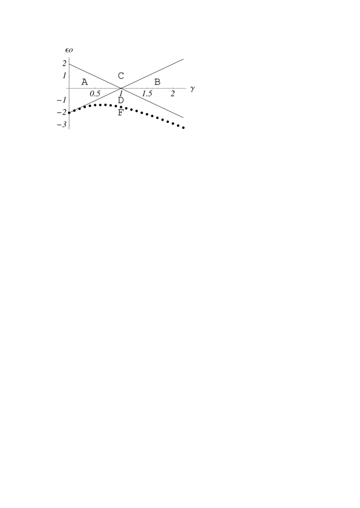
FIG. 1.: $\epsilon_{0}-\gamma$ phase diagram for the single impurity case.

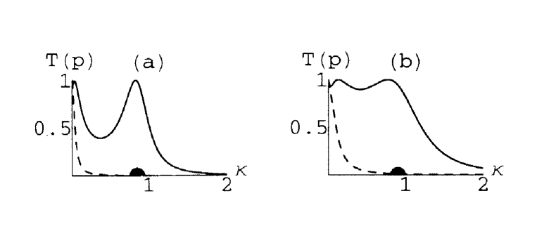
FIG. 2.: The transmission $T$ as function of $\kappa$ (in units of the cutoff $\omega$), for $U=5\hbar^{2}/(2m)$. The solid line is $T(p)$, the dashed line shows $|t_{p}|^{2}$. (a) $p=0.04\omega$, (b) $p=0.1\omega$.

REFERENCES

- [1] B. L. Altshuler and A. G. Aronov, in Electron-Electron Interactions in Disordered Systems, A.L. Efros and M. Pollak, eds. p. 1-154, North Holland, Amsterdam (1985); A. M. Finkelstein, Sov. Phys. JETP 67, 97 (1983).
- [2] D. L. Shepelyansky, Phys. Rev. Lett. 73, 2607 (1994).
- [3] F. von Oppen, T. Wettig and J. Müller, Phys. Rev. Lett. 76, 491 (1996).
- [4] M. Ortuño and E. Cuevas, Europhys. Lett. 46, 224 (1999).
- [5] L. P. Kouwenhoven et al., Mesoscopic Electron Transport, Proceedings of the NATO Advanced Study Institute, edited by L. L. Sohn, L. P. Kouwenhoven and G. Schön (Kluwer 1997); M. A. Kastner, Comm. Cond. Mat. 17, 349 (1996); R. Ashoori, Nature 379, 413 (1996); L. P. Kouwenhoven et al., Phys. Rev. Lett. 65, 361 (1990).
- [6] G. Grabert and M.H. Devoret (eds) Single Charge Tunneling, Coulomb Blockade Phenomena in Nanostructures, Nato ASI, Series B: Physics, vol 294. Plenum, NY (1992).
- [7] T. K. Ng and P. A. Lee, Phys. Rev. Lett. 61, 1768 (1988).
- [8] P. W. Anderson, Phys. Rev. 124, 41 (1961).
- [9] A. Yacoby et al., Phys. Rev. Lett., 74, 4047 (1995).
- [10] R. Berkowits, Phys. Rev. Lett. 73, 2067 (1994).
- [11] e. g. R. H. Blick et al., Phys. Rev. Lett. 80, 4032 (1998); G. Schedelbeck et al., Science 278, 1792 (1997).
- [12] N. B. Zhitenev, R. C. Ashoori, L. N. Pfeiffer and K. W. West, Phys. Rev. Lett. 79, 2308 (1997).
- [13] For a recent discussion, see, e.g., H. Ness and A. J. Fisher, cond-mat/9903320.
- [14] A. Aharony, O. Entin-Wohlman, and Y. Imry, cond-mat/9904182.