[

The spectral weight of the Hubbard model through cluster perturbation theory

Abstract

We calculate the spectral weight of the one- and two-dimensional Hubbard models, by performing exact diagonalizations of finite clusters and treating inter-cluster hopping with perturbation theory. Even with relatively modest clusters (e.g. 12 sites), the spectra thus obtained give an accurate description of the exact results. Thus, spin-charge separation (i.e. an extended spectral weight bounded by singularities) is clearly recognized in the one-dimensional Hubbard model, and so is extended spectral weight in the two-dimensional Hubbard model.

]

One of the central issues in the theory of strongly correlated electrons is the existence or not of well-defined quasiparticles. This question is best addressed by studying the spectral weight (SW) $A({\bf k},\omega)$, i.e., the probability distribution for the energy $\hbar\omega$ of an electron of wavevector ${\bf k}$ added to, or removed from the system. In a Fermi liquid, the SW is dominated by a single quasiparticle peak centered at $\omega=\varepsilon({\bf k})$, whose width decreases as $\varepsilon({\bf k})$ approaches the Fermi energy. In a Luttinger liquid, the SW is distributed between two singularities associated respectively to spin and charge excitations (spinons and holons)[1]. The hole (i.e., electron-removal) part of the SW can be measured by angle-resolved photoemission spectroscopy (ARPES), a technique which has improved steadily in recent years[2, 3, 4]. On the theoretical side, the SW is obtained from the one-particle Green function:

$$A({\bf k},\omega)=\lim_{\eta\to 0^{+}}-2\>{\rm Im}\>{\cal G}({\bf k},\omega+i\eta),$$ (1)

and the latter may be approximately evaluated by various analytical and numerical methods.

In this letter we explain a new method for calculating $A({\bf k},\omega)$ in Hubbard-type models, based on a combination of exact diagonalizations (ED) of finite clusters with strong-coupling perturbation theory[5, 6], and apply it to the one- and two-dimensional Hubbard models. Exact diagonalizations based on the Lanczos algorithm are commonly used to evaluate $A({\bf k},\omega)$[7, 8, 9, 10]. Unfortunately, computer memory requirements grow exponentially with system size and restrict the analysis to small clusters (e.g. 16 sites for the Hubbard model). The SW thus obtained is the sum of a relatively small number of poles and its extended character in the thermodynamic limit is difficult to assess. The SW may also be evaluated by quantum Monte Carlo (QMC)[11, 12, 13, 14]: larger systems may thus be studied (e.g. 64 sites) but the maximum entropy method (MEM) used for approximate analytic continuation tends to produce smooth SW and may miss weak features; moreover, computation time increases as the temperature is lowered. The new method we propose consists in (i) dividing the lattice into identical $N$-site clusters; (ii) evaluating – by ED – the one-particle Green function $G_{a,b}(z)$ within a cluster ($a,b$ are lattice sites and $z$ a complex frequency) with open boundary conditions; (iii) treating the inter-cluster hopping $t_{0}$ in perturbation theory and recovering the Green function ${\cal G}({\bf k},\omega)$. Thus, short-distance effects are treated exactly, while long-distance propagation is treated at the RPA level.

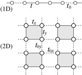
FIG. 1.: Dividing the lattice into identical four-site clusters for the 1D and 2D Hubbard models. The in-cluster hopping amplitude is $t$ and the inter-cluster hopping is $t_{0}$.

Step (i) is illustrated on Fig. 1. We denote by $t$ and $t_{0}$ the hopping amplitudes within and between clusters, respectively ($t$ and $t_{0}$ may be different a priori, but will be identical in practice). Clusters of up to $N=12$ sites have been treated, with various aspect ratios in the 2D case. Open (free) boundary conditions must be used. Step (ii) proceeds according to the usual Lanczos method[7]. The cluster Green function $G_{a,b}(z)$ is defined as

$$G_{a,b}(z)=\L\Omega|c_{a}{1\over z-H}c^{\dagger}_{b}|\Omega\rangle+\L\Omega|c^{\dagger}_{b}{1\over z+H}c_{a}|\Omega\rangle$$ (2)

where $|\Omega\rangle$ is the ground state obtained by ED, $c_{a}$ is the electron destruction operator at site $a$ (we drop the spin index) and $H$ is the Hamiltonian (including chemical potential). The two terms in $G_{a,b}$ correspond respectively to electron ($G_{a,b}^{\rm e}$) and hole ($G_{a,b}^{\rm h}$) propagation, and are calculated separately. In the subspace containing one additional electron (with respect to the ground state), an accurate tridiagonal representation of $H$ is obtained (typically of dimension ranging from 50 to 250). Efficient routines for inverting tridiagonal matrices are used to evaluate $G_{a,b}^{\rm e}(z)$ at any desired complex value, and likewise for $G_{a,b}^{\rm h}(z)$. In usual Lanczos calculations, this inversion takes the form of a continued-fraction representation.

Step (iii) demands more explanations. Let $c_{m,a}$ be the electron destruction operator on site $a$ of cluster $m$ ($a=1,\dots,N$). The full system is treated as a superlattice of clusters, each cluster being made of $N$ ordinary lattice sites; we will work in one dimension for simplicity, but a suitable generalization to higher-dimensional lattices is readily obtained. The complete Hamiltonian of the system may be written as $H=H_{0}+V$:

$$H_{0}=\sum_{m\in{\mathbb{Z}}}H^{0}_{m}\quad,\quad V=\sum_{\scriptstyle m,n\atop\scriptstyle a,b}V^{m,n}_{a,b}c_{m,a}^{\dagger}c_{n,b}$$ (3)

where $H^{0}_{m}$ is, say, the Hubbard Hamiltonian of the $m^{\rm th}$ cluster

$$H^{0}_{m} = -t\sum_{\L a,b\rangle}\sum_{\sigma}\l(c^{\dagger}_{m,a,\sigma}c_{m,b,\sigma}+{\rm H.c.}\right)$$ (5)

$$\qquad+U\sum_{a}n_{m,a,\uparrow}n_{m,a,\downarrow}$$

and $V$ is the nearest-neighbor hopping between adjacent clusters:

$$V^{m,n}_{a,b}=-t_{0}(\delta_{m,n-1}\delta_{a,N}\delta_{b,1}+\delta_{m,n+1}\delta_{a,1}\delta_{b,N})$$ (6)

Of interest is the electron Green function ${\cal G}_{a,b}(Q,z)$, where $Q$ is a superlattice wavevector, and $a,b$ are site indices within a cluster. The perturbation $V$ being a one-body operator, it may be treated in the formalism of Refs [5, 6], wherein a systematic perturbation expansion was constructed for such terms. The lowest-order contribution to this expansion has the RPA form:

$${\cal G}_{a,b}(Q,z)=\l({{\hat{G}}(z)\over 1-{\hat{V}}(Q){\hat{G}}(z)}\right)_{a,b}$$ (7)

where ${\hat{G}}(z)$ is the generalization of the “atomic” Green function, now a $N\times N$ matrix in the space of site indices. Likewise, ${\hat{V}}(Q)$ is the reciprocal superlattice representation of the hopping (6):

$$V_{a,b}(Q)=-t_{0}\l({\rm e}^{iQ}\delta_{a,N}\delta_{b,1}+{\rm e}^{-iQ}\delta_{a,1}\delta_{b,N}\right)$$ (8)

Relation (7) may be regarded as a cluster generalization of the Hubbard-I approximation[15].

The Green function ${\cal G}_{a,b}(Q)$ of Eq. (7) is in a mixed representation: real space within a cluster and Fourier space between clusters. A true Fourier representation in terms of the original reciprocal lattice is preferred. Since the cluster decomposition breaks translation invariance, ${\cal G}$ will depend on two continuous momenta $k$ and $k^{\prime}$, identical modulo a reciprocal superlattice vector:

$${\cal G}(k,k^{\prime};z) = {1\over N}\sum_{s=0}^{N-1}\delta\l(k-k^{\prime}+{2\pi s\over N}\right)$$ (10)

$$\quad\times\sum_{a,b=1}^{N}{\rm e}^{-ik(a-b)}{\rm e}^{2\pi isb/N}{\cal G}_{a,b}(Nk,z)$$

If we set $t=t_{0}$, the $s=0$ component ($k=k^{\prime}$) is the RPA approximation to the full Green function:

$${\cal G}_{\rm RPA}(k,z)={1\over N}\sum_{a,b}{\rm e}^{-ik(a-b)}{\cal G}_{a,b}(Nk,z)$$ (11)

Eqs (7,11) are then used to calculate the SW.

The approximation (7) turns out to be exact in the absence of interactions ($U=0$). In that case, Wick’s theorem applies and the RPA form is the exact resummation of the perturbation series, ${\hat{V}}(Q)$ being the exact self-energy. If we set $t=t_{0}$, Eq. (11) then yields the exact Green function for an infinite system at arbitrary wavevector, from the exact Green function $G$ of an finite, open cluster. When $U\neq 0$, Expression (11) is no longer exact, but strong interactions tend to cause short-range correlations that are incorporated with good accuracy in modest-size clusters. Thus short-distance effects are well served by the ED within a cluster, and long-distance effects by the RPA approximation, making our method adequate at intermediate coupling.

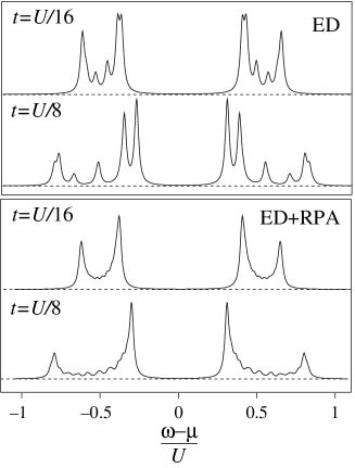
FIG. 2.: Above: $A(\pi/2,\omega)$ for the 1D Hubbard model at half-filling on a 12-site ring with ordinary ED. Below: the same, but with applying RPA with 12-site clusters. The extended character of the SW is manifest. Note: the parameter $\eta$ of Eq. (1) has been set to 0.03 in order to give delta peaks a finite width.

We have applied the method just described to the 1D Hubbard model. Fig. 2 compares the result of an ordinary ED on a 12-site ring with the present approach: Whereas the extended character of $A(k,\omega)$ – here a signature of spin-charge separation – is not clear form the ED data alone, it is clearly revealed by the RPA spectra. In fact, the two branches of the SW can already be seen with a two-site cluster (not shown), but more and more poles appear in between when the cluster size is increased: the actual separation of spin and charge excitations needs a fair cluster size to occur, and propagation between clusters at the RPA level requires the holon and spinon to recombine.

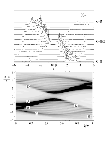
FIG. 3.: Spectral weight of the 1D Hubbard model at half-filling, for $U=4t$, calculated from Eqs. (7) and (11) with $N=12$. Below, density plot of the same data.

Fig. 3 illustrates the SW of the 1D Hubbard model at half-filling with $U/t=4$. Most noteworthy are: (i) The extended character of the SW, with six branches having a clear dispersion, even though most of the weight lies near the “quasiparticle band” following approximately the $-2t\cos k$ free-particle dispersion; (ii) the gap opening at $k=\pi/2$; (iii) the spinon (A) and holon (B) branches, characteristic of a Luttinger liquid with a charge gap (Branch D is the mirror of the holon branch with opposite frequency)[16]; (iv) the weak, higher-frequency band (C), absent from low-energy Luttinger liquid predictions; (v) the high-frequency tail (E) near the zone boundary. Band C, as well as Bands B and D together, disperse with period $\pi$ instead of $2\pi$, a signature of local AF correlations. A comparison with Fig. 1c of Ref. [10] – which illustrates the SW in the $U\to\infty$ limit – is revealing of the changes brought about by a finite value of $U$: in the $U\to\infty$ limit, just the hole part of the SW is present, but the same branches can be found, however with comparable relative intensity: Branches D and E are the mirror images of branches B and A, respectively. The finite value of $U$ weakens considerably the intensity of branches C, D, and E. It is also interesting to compare Fig. 3 with Fig. 2 of Ref. [12] and Fig. 3 of Ref. [5], where the same parameters were used. In particular, it is clear that the Maximum Entropy Method of Ref. [12] lumps the spinon and holon peaks near $k=0$ into one broad peak.

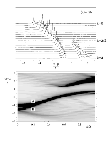
FIG. 4.: Spectral weight of the 1D Hubbard model at $\L n\rangle={5\over 6}$ and $U=4t$, calculated from Eqs. (7) and (11) with $N=12$. Below: density plot of the same data.

Fig. 4 shows the SW of the 1D Hubbard model for the same value of $U/t$, but away from half-filling, at $\L n\rangle={5\over 6}$. The chemical potential $\mu=0.64$ was inferred from the integrated density of states. The Fermi level crosses the main band, causing metallic behavior, but again the SW is clearly extended, with a clear weakening of the upper Hubbard band: there is a significant transfer of SW from high to low frequencies[17]. Again, the spinon (A) and holon (B) branches are clearly identified, this time in a gapless Luttinger liquid. This may be compared with Fig. 3 of Ref. [14], which corresponds to the same $U/t$ ratio, but with $\L n\rangle={3\over 4}$.

We have also applied our method to the 2D Hubbard model, with various cluster shapes ($2\times 6$, $3\times 4$, $4\times 3$ and $6\times 2$). The spectra obtained from these different shapes are very similar, and this reinforces our confidence in them, even though the linear dimensions of the clusters are modest. Fig. 5 illustrates the SW of the 2D Hubbard model at half-filling for $U=8t$, with a $3\times 4$ cluster. This is to be compared with Fig. 1 of Ref. [13] and Fig. 6 of Ref. [6]. In contrast to the 1D case, the SW is much more concentrated around one peak, but its extended character is still undeniable. Indeed, one is tempted to draw an analogy with 1D spinon and holon branches: the momentum scan $\rm\Gamma-X-M$ shares features with the $[0,\pi]$ scan in the 1D case, except that the “spinon” (A) is much weaker than the “holon” (B). The same can be said of the diagonal scan $\rm\Gamma-M$ (from right to left on Fig. 5). Likewise, a high-frequency band (C) is visible. Most obvious is the gap opening at the Fermi surface, constant along the XY line, a feature that would certainly be modified by including a diagonal hopping $t^{\prime}$, and which demonstrates anyway that nearest-neighbor hopping alone cannot account for the ARPES data of insulating cuprates[4] (this was already known for the $t-J$ model). Note, that whereas Refs. [13] and[6] both resolve two peaks near Point M, the present approach suggests an extended SW at that point. The expected antiferromagnetic order of the half-filled 2D Hubbard model is not seen here, because of finite cluster size. This order would imply a folding of the Brillouin zone, with a corresponding symmetry of the SW following the SDW fit illustrated on Fig. 5.

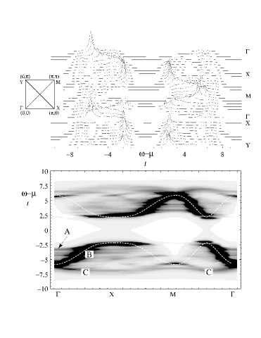
FIG. 5.: Spectral weight of the 2D Hubbard model at half-filling, for $U=8t$, calculated from Eqs. (7,11) with a $3\times 4$ cluster. Inset: The wavevector scans. Below: density plot of the same data (except for the scan from X to Y) to be compared directly with Fig. 1 of Ref. [13]. The dashed curve is the best SDW dispersion, with $t=1.36$ and gap $\Delta=2.21$.

Some general remarks are in order. Formulas (7,11) are but the first order result of a systematic $t_{0}$ expansion (See Ref. [6] for details). It is difficult to assess the convergence of this perturbative expansion, since it depends certainly on the ratio $t/U$ and on cluster size $N$. We expect nonetheless the method to give better results at strong coupling, where short-range effects dominate and are thus well accounted for by modest clusters. Indeed, the effect of antiferromagnetic correlations are already seen with two-site clusters. Going to order $t_{0}^{2}$ in strong-coupling perturbation is a way of improving the results presented here, but appears quite difficult in practice, because of the need to compute numerically exact two-particle Green functions on a cluster. The spectra presented here are all normalized, up to 1 or 2%. The general form (7) guarantees that the continued fraction form of the SW will have the correct first coefficient, thus ensuring its normalization.

In summary, we have shown how strong-coupling perturbation theory can be used to incorporate long-distance effects into ED data which already contain short-distance effects exactly. This method allows for a clear recognition of spin-charge separation in the 1D Hubbard model, and of extended SW in the 2D Hubbard model. Further applications of this method (NNN hopping, three-band Hubbard model, etc.) are under way.

We thank S. Pairault and A.-M. S. Tremblay for numerous enlightening discussions. This work was partially supported by NSERC (Canada) and FCAR (Québec).

REFERENCES

- [1] J. Voit, Rep. Prog. Phys. 57, 977 (1994).
- [2] C. Kim et al., Phys. Rev. Lett. 77, 4054 (1996).
- [3] C. Kim et al., Phys. Rev. Lett. 80, 4245 (1998).
- [4] F. Ronning et al., Science 282, 2067 (1998).
- [5] S. Pairault, D. Sénéchal, and A.-M. S. Tremblay, Phys. Rev. Lett. 80, 5389 (1998).
- [6] S. Pairault, D. Sénéchal, and A.-M. S. Tremblay, cond-mat/9905242 (unpublished).
- [7] E. Dagotto, Rev. Mod. Phys. 66, 763 (1994).
- [8] P. Leung et al., Phys. Rev. B 46, 11779 (1992).
- [9] Y. Otha et al., Phys. Rev. B 46, 14022 (1992).
- [10] J. Favand et al., Phys. Rev. B 55, R4859 (1997).
- [11] N. Bulut, D. Scalapino, and S. White, Phys. Rev. B 72, 705 (1994).
- [12] R. Preuss et al., Phys. Rev. Lett. 73, 732 (1994).
- [13] R. Preuss, W. Hanke, and W. von der Linden, Phys. Rev. Lett. 75, 1344 (1995).
- [14] M. Zacher, E. Arrigoni, W. Hanke, and J. Schrieffer, Phys. Rev. B 57, 6370 (1998).
- [15] J. Hubbard, Proc. Royal. Soc. London 276, 238 (1963).
- [16] J. Voit, in Proceedings of The Ninth International Conference on Recent Progress in Many-Body Theories, Sydney, edited by D. Neilson (World Scientific, Singapore, 1998).
- [17] M. Meinders, H. Eskes, and G. Sawatzky, Phys. Rev. B 48, 3916 (1993).