Spin Chains in an External Magnetic Field.Closure of the Haldane Gap and Effective Field Theories.

Abstract

We investigate both numerically and analytically the behaviour of a spin-1 antiferromagnetic (AFM) isotropic Heisenberg chain in an external magnetic field. Extensive DMRG studies of chains up to $N=80$ sites extend previous analyses and exhibit the well known phenomenon of the closure of the Haldane gap at a lower critical field $H_{c_{1}}.$ We obtain an estimate of the gap below $H_{c_{1}}$. Above the lower critical field, when the correlation functions exhibit algebraic decay, we obtain the critical exponent as a function of the net magnetization as well as the magnetization curve up to the saturation (upper critical) field $H_{c_{2}}.$ We argue that, despite the fact that the $SO(3)$ symmetry of the model is explicitly broken by the field, the Haldane phase of the model is still well described by an $SO(3)$ nonlinear $\sigma$-model. A mean-field theory is developed for the latter and its predictions are compared with those of the numerical analysis and with the existing literature.

]

I Introduction.

Spin chains, ladders and, more generally, low-dimensional quantum spin systems have become a subject of considerable theoretical and (more recently) experimental interest [1]. This has been due in the recent past to the connection that 2D AFM Heisenberg models have with the $Cu-O$ planes in the new ceramic superconducting materials [2], but spin chains and ladders have become rapidly a subject of autonomous interest in their own.

Back in the early $80$’s Haldane [3] put forward his by now famous “conjecture” according to which half-odd-integer AFM Heisenberg spin chains should have a gapless spectrum, and hence be critical at $T=0$ with algebraic decay of correlations while integer spin chains should be gapped with exponential decay of correlations. The conjecture is based on the presence, in the effective action that, in the continuum limit, maps the chain onto a ($1+1$) nonlinear Sigma model [$NL\sigma M$] [4], of a topological term (basically a Pontrjagin index [4, 5, 6, 7]), that is effective only when the spin is half-odd-integer (for details see, e.g. [1]). It was later proved rigorously [8] that a ($1+1$) $NL\sigma M$ without topological terms has a unique ground state and is gapped with an excitation spectrum consisting of a triplet of massive bosons, as well as that the topological term makes the model gapless [9]. This implies of course that all half-odd-integer spin chains fall into the same universality class of the spin-$1/2$ chain, whose exact solution is well established by the Bethe-Ansatz [10, 11], and that is known to be gapless. Were it not for the presence of the topological term, the description of half-odd-integer spin chains in terms of effective nonlinear $\sigma$ model [NL$\sigma$M] actions would lead then to predictions in blatant disagreement with the results of the Lieb-Schultz-Mattis [LSM] theorem [12], which predicts a (non Goldstone) gapless sector in the excitation spectrum in the presence of a unique ground state. All this applies to systems with translationally- (and parity)-invariant couplings. Gapfull half-odd-integer spin chains can occur when these invariances are explicitly broken [1].

The conclusions of LSM do not apply to integer-spin chains, though, and there a unique ground state and a gap (the “Haldane gap”) may well coexist. Indeed, neutron-scattering measurements on quasi one-dimensional compounds [13] have established the presence of the Haldane gap in a class of integer-spin systems. Also, a rigorous example of an $S=1$ model with a gapped unique ground state has been exhibited (among other rigorous results) in a seminal paper by Affleck et al. [14].

In more recent years there has arisen a growing interest in the behaviour of spin chains and/or ladders in an external (uniform and/or staggered [15]) static magnetic field. Actually, the magnetization curve of the spin one-half AFM Heisenberg chain had been studied already by Griffiths back in the early Sixties [16]. The main result of Ref.[16] was that the magnetization $m$ per site, as a function of the external field $H$, grows steadily from $H=0$ (with a finite slope corresponding to a finite initial susceptibility, as expected) to the saturation value of $m=$ $S=1/2$. The latter is reached at an upper critical field $H_{c_{2}}$ given by (absorbing the Bohr magneton and the spin $g$-factor in the definition of the field): $H_{c_{2}}=4SJ=2J$ for $S=1/2$ ($J$ being the AFM exchange constant) with infinite slope: $S-m\propto(H_{c_{2}}-H)^{1/2}$. A continuous (in the thermodynamic limit) change of the magnetization as a function of the applied field implies of course that there are no gaps in the spectrum towards excitations from a value of the spin to a neighboring one. The $S=1/2$ model remains therefore gapless from $H=0$ up to $H=H_{c_{2}}$, where the ground state becomes fully polarized. In this connection, it should be mentioned that the opposite phenomenon, namely a field-induced gap has been observed [17] in neutron-scattering experiments on what can be considered as a (quasi) one-dimensional $S=1/2$ spin system, namely $Cu$ benzoate. It has however been argued convincingly [18] that this is possible only in the presence of various types of anisotropies, leading to an effective internal staggered field (see [18] for more details).

As already stated, integer-spin (isotropic) AFM chains are in a gapped “Haldane” phase at zero field. This appears to be true [19] also for XXZ models, i.e. for more general model Hamiltonians of the form:

$${\cal H=}J\sum_{i=1}^{N}\left\{\lambda S_{i}^{z}S_{i+1}^{z}+\frac{1}{2}(S_{i}^{+}S_{i+1}^{-}+S_{i}^{-}S_{i+1}^{+})\right\}$$ (1)

for a chain of $N$ sites (we don’t specify here boundary conditions (see [19] for details)), where $\lambda\geq 0$ is an anisotropy parameter in a range that includes the (exactly soluble, $\lambda=0$) $XY$ model, the (isotropic, $\lambda=1$) Haldane phase as well as, for $\lambda>1$, uniaxial Ising-like phases.

Sticking for the time being to the isotropic, $\lambda=1$ case, and according to the analysis of [8], the lowest excited state is a triplet of massive, $S=1$ bosons. In the absence of an external magnetic field the latter are degenerate and separated from the ground state by a finite energy gap $\Delta_{0}.$ The addition to the model of an interaction with an external field leads to new and interesting phenomena.

As observed by Affleck [20], the Zeeman splitting due to the field will cause one of the branches of the spectrum to lower its energy. The gap will remain “robust” (and the magnetization will remain zero) up to a lower critical field: $H_{c_{1}}=\Delta_{0}$, when the lower branch of the spectrum will cross the ground state. At this point, a “Bose condensation of magnons” [21] should take place, and the spectrum should become gapless. This implies of course that the magnetization should remain zero for fields up to the lower critical field, while it should rise to the saturation value at some upper critical field $H_{c_{2}}\geq H_{c_{1}}$. The value $H=H_{c_{1}}$ of the field is then the one that leads to the closure of the Haldane gap in the excitation spectrum. Parenthetically, it should be remembered that the existence, for integer spins, of a lower critical field leading to the closure of the Haldane gap had already been predicted previously by Schulz [22].

The Lieb-Schultz-Mattis Theorem [12], originally formulated in zero external field, has been generalized to both spin chains [23, 21] and ladders [24] in the presence of a field. The main results of [21] for spin chains (but see also [24] for a generalization) are that, in the presence of a field:

i) If translational symmetry is not broken, then the ground state for a spin-$S$ chain is gapless unless the magnetization per site $m$ obeys the “quantization condition”:

$$S-m\in Z,\text{ an integer}$$ (2)

This implies that gaps in the spectrum, and hence plateaus in the magnetization curve can (but in principle need not, of course) be present when the above “integer quantization” condition is met. Moreover:

ii) “Fractional quantization” (completing an overall scenario that resembles closely [21] that of the (integer and fractional) Quantum Hall Effect), i.e.: $S-m=$ half-odd-integer, may lead to additional “fractional” plateaus accompanied, however, by spontaneous breaking of the translational symmetry of the ground state.

Although plateaus (both integer and fractional) are not forbidden at quantized values of the magnetization, whether or not they do actually occur depends very much on the details of the model. For $S=1$ the only admissible gaps are at $m=0$ (with a width: $H_{c_{1}}\approx\Delta_{0}$, the Haldane gap) and (trivially) at $m=S=1$ for $H\geq H_{c_{2}}$, corresponding to the fully polarized state. In order to have gaps at intermediate values one needs therefore $S\geq 3/2$. The existence of a gap at $m=1/2$ has been proved by Tasaki [25] and numerically found [21, 26] only in the presence of a strong single-ion anisotropy. Some numerical [24] and experimental [27] evidence of magnetization plateaus has been reported for $S=1/2$ (even-legged) spin ladders.

We will restrict ourselves from now on to the case of $S=1$ AFM isotropic Heisenberg chains. For these systems the magnetization is supposed to rise continuosly for $H_{c_{1}}\leq H\leq H_{c_{2}}$ from zero to saturation. The model being gapless in this range of fields, the transverse spin-spin correlation function (e.g.: $\langle S_{0}^{x}S_{r}^{x}\rangle$ if the external field $H$ is in the $z$-direction) is expected to decay algebraically: $\langle S_{0}^{x}S_{r}^{x}\rangle\propto(-1)^{r}r^{-\eta}$ with some critical exponent $\eta$. Affleck [20] has suggested that the ground state above $H_{c_{1}}$ should be regarded as a Bose condensate of low-energy bosons and has proposed an effective Ginzburg-Landau-type field theory to describe the system near the transition. His predictions are that $\eta$ should exhibit the universal behaviour: $\eta\simeq 1/2$ near $H_{c_{1}}$ and that the induced magnetization should vanish in a nonanalytic way at $H_{c_{1}}$, namely: $m\propto\sqrt{H-H_{c_{1}}\text{ }}$for $H\gtrsim H_{c_{1}}$. This prediction seems to be reasonably well supported by numerical findings [28]. In the same reference it was also inferred from the numerical data that $\eta\approx 1/2$  as well when $H\rightarrow H_{c_{2}}$. It is unclear whether such a prediction can be actually extracted firmly from the available numerical data.

The motivations of the present paper are twofold: we wanted to extend and to put on firmer bases the existing numerical analyses of the model, which has proven to be possible by a systematic use of the DMRG that has allowed us to analyze samples with an higher number of sites (up to $N=80$) than down hitherto, and to try and understand the Haldane phase in terms of an appropriate effective field theory.

The plan of the paper is as follows: In Sect. II we give the details of the numerical procedure followed in the study (at $T=0$) of finite samples and report the results for the Haldane gap, the critical fields, the magnetization curve and the critical exponent for the (transverse) spin-spin correlation function. In Sect. III we discuss, at the mean field level, the predictions of an effective field theory based on the $O(3)$ nonlinear $\sigma$ model (NL$\sigma$M) for the Haldane phase of the chain, comparing the predictions of the theory with the numerical results. Sect. IV is devoted to a brief discussion and to the conclusions.

II Numerical Results

The Hamiltonian we consider here is:

$${\cal H}=J\sum\limits_{\langle ij\rangle}{\bf S}_{i}\cdot{\bf S}_{j}-H\sum\limits_{i}S_{i}^{z}$$ (3)

where: S${}_{i}^{2}=S(S+1)$, $S=1$ (we set $\hbar=1$ from now on), the sums run over a chain of $\ N=L/a$ spins, $L$ being the length of the chain and $a$ the lattice spacing. $J$ is the AFM coupling between nearest-neighboring spins and $H$ (which includes factors such as Bohr magneton, gyromagnetic factor and the like) is a static and uniform external magnetic field pointing in the $z$-direction. Here and in the rest of the paper we shall assume periodic boundary conditions (PBC’s).

We have employed the standard DMRG algorithm [29, 30, 31, 32] to calculate the magnetization curve and the static transverse spin-spin correlation function:

$$G^{xx}(r)=\langle S_{r}^{x}S_{0}^{x}\rangle$$ (4)

($r=j$, in units of $a$ with $j$ an integer, $0\leq j\leq N$). From the latter one can extract both the value of the correlation length (and hence of the spin gap) in the Haldane phase and, as a function of, e.g., the magnetization, the critical exponent governing the algebraic decay of correlations in the gapless phase. We have adopted a finite-chain “zip” algorithm which increases considerably the precision of the resulting data, though of course at the price of an increase in computer time. In the whole of this Section we measure energies in units of $J$, i.e. we set $J=1$.

FIG. 1.: a) The hystogram of the magnetization curve for $N=32$ spins. b) Continuous interpolation of the data in Fig. 1-a. See text for details.

The hystogram of the magnetization for $N=32$ spins is reported in Fig. 1-a, while Fig. 1-b represents a continuous interpolation of the data. The curve in Fig. 1-b passes through the midpoints of the plateaus of the hystogram and is an indication of what the magnetization curve should look like in the thermodynamic limit $N\to\infty.$

The magnetization remains zero up to a lower critical field of $H_{c_{1}}=0.412232$ (in our units). Identifying $H_{c_{1}}$ with $\Delta_{0}$, $\Delta_{0}$ being the spin gap, this is a close upper limit to the $N\to\infty$ extrapolations [29] that give: $\Delta_{0}/J$=$0.40450(2).$ Similar results have been reported also by Golinelli et al. [33]. Above the lower critical field the magnetization increases steadily until it saturates at the upper critical field $H_{c_{2}}/J=4$ (equal to $4S$ for $S=1$). From the data of Fig.$1$, it emerges that the numerical analysis reproduces in a completely nonambiguous way the singular square-root behaviour of the magnetization near the upper critical field. The data are also consistent with a similar square-root vanishing [20] of the magnetization when the lower critical field is approached from above, but seem to indicate that the low-field singular behaviour sets in in a much narrower range of fields than the one near $H_{c_{2}}$. The values of $(-1)^{r}G^{xx}(r)$ are plotted in Fig. 2 for a chain of $N=64$ spins and $H<H_{c_{1}}$. PBC’s make of course the curve symmetric around $N/2=32$. The data are well fitted, taking PBC’s into account, by a curve of the form:

$$(-1)^{r}G^{xx}(r)=A\left\{\frac{e^{-r/\xi_{0}}}{\sqrt{r}}+\frac{e^{-(N-r)/\xi_{0}}}{\sqrt{N-r}}\right\}$$ (5)

with:

$$A=1.07508,\text{ \ }\xi_{0}=6.08304$$ (6)

both independent of the field up to $H=H_{c_{1}}$. The form of $G^{xx}(r)$ reported here corresponds to the (symmetrized) asymptotic behaviour of the modified Bessel function [34] $K_{0}(r/\xi),$ which is the form of the spin-spin static correlation function predicted by the continuum theory to be discussed in the next Section. Also, defining the spin-wave velocity $c$ as: $c=\Delta_{0}\xi$ ($\Delta_{0}\xi/\hbar$ if we reinstate Planck’s constant into its proper place) we find $c\simeq 2.4$ in units of $Ja$ (or $Ja/\hbar$). The continuum theory (see below) predicts instead $c=2$ (for $S=1$ and in the same units). The discrepancy may be attributed both to the approximations involved in performing the continuum limit and to finite-size effects that may affect the numerical estimates.

FIG. 2.: A plot of $(-1)^{r}G^{xx}(r)$ ($r=j$, in units of $a$, where $j$ is an integer) for a chain of $N=64$ spins and $H<H_{c_{1}}$. The points are the numerical data and the continuous curve is the interpolation with the analytic form of Eq.(5).

For $H_{c_{1}}\leq H\leq H_{c_{2}}$ the correlation function is expected to exhibit an asymptotic algebraic decay, i.e. to behave asymptotically as:

$$(-1)^{r}G^{xx}(r)\approx\frac{1}{r^{\eta}}+\frac{1}{(N-r)^{\eta}}$$ (7)

Here too the second term accounts for the PBC’s and $\eta=\eta(m).$ According to Moreo[35] and to Sakai and Takahashi[28] the most efficient way to calculate $\eta$ goes through the evaluation of the (staggered) structure factor:

$$S_{N}=\sum\limits_{r=1}^{N-1}\exp\{ikr\}G^{xx}(r)|_{k=\pi}$$ (8)

A power-law behaviour as in Eq.(7) implies: $S_{N}\approx N^{1-\eta}$ for large $N,$ and one obtains the critical exponent as:

$$\eta(m)=1-\frac{\ln\left(S_{N}/S_{M}\right)}{\ln\left(N/M\right)}$$ (9)

with the most reliable values being obtained for the highest $M,N$ available.

In Fig.$3$ we report our numerical results for $\eta$ together with some interpolations. The data have been obtained by employing about eight runs for each value always using the “zip ” algorithm twice and keeping between $190$ and $234$ states in the reduced density matrix. The longest chains studied here have up to $N=80$ spins.

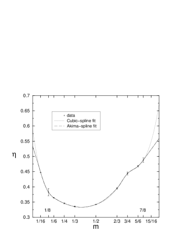
FIG. 3.: The crtitical exponent $\eta$ (see Eq.(7)) as a function of the magnetization for chains up to $N=80$ spins. The interpolating curves should be taken mainly as guides for the eye.

For $m\to 0$ we obtain extrapolated values of $\eta$ slightly above the theoretical prediction [20] of $\eta=1/2$. This may be due to uncertainties in the interpolation scheme and again to finite-size effects. For $m\to 1$, i.e. near saturation, our data seem to be consistent with a finite limiting value of $\eta$ at saturation.

Our numerical results indicate that the system remains in the Haldane phase for fields up to $H_{c_{1}}$, while it becomes (quantum) critical for higher fields when a nonzero magnetization develops. In the next Section we will try to set up a consistent field-theoretical description of the Haldane phase.

III Effective Field Theory for the Haldane Phase

That AFM Heisenberg spin chains can be mapped, in the continuum limit, into O(3) NL$\sigma$ models was shown for the first time by Haldane [3] and such “Haldane maps” have been widely used since. As the procedure is by now well known, we summarize here only its main points.

In order to use the partition function as a generating functional for (Euclidean) Greeen functions, we will replace for the time being the Hamiltonian of Eq.(3) with:

$${\cal H}=J\sum\limits_{\langle ij\rangle}{\bf S}_{i}\cdot{\bf S}_{j}-\sum_{i}{\bf B}_{i}\cdot{\bf S}_{i},\text{ }J>0$$ (10)

where ${\bf B}_{i}$ is an external site- and possibly time-dependent magnetic field. Here too PBC’s will be assumed throughout.

The (canonical) partition function can be written in a standard manner as a path integral over spin coherent states as:

$${\cal Z}=\int[{\cal D}{\bf\Omega}]\delta({\bf\Omega}^{2}-1)\exp\{-{\cal S}_{E}\}$$ (11)

where the (Euclidean) action is given by:

$${\cal S}_{E}={\cal S}_{WZ}+\int\limits_{0}^{\beta}{\cal H}[{\bf\Omega}(\tau)]d\tau$$ (12)

${\bf\Omega}$ is a classical vector field of unit magnitude,

$${\cal H}[{\bf\Omega}(\tau)]=JS^{2}\sum\limits_{\langle ij\rangle}{\bf\Omega}_{i}(\tau)\cdot{\bf\Omega}_{j}(\tau)-S\sum_{i}{\bf B}_{i}(\tau)\cdot{\bf\Omega}_{i}(\tau)$$ (13)

and ${\cal S}_{WZ}$ is the Wess-Zumino part of the action given by:

$$S_{WZ}=is\sum_{i}\int_{0}^{\beta}\,d\tau[1-\cos\theta_{i}(\tau)]\,{\dot{\phi}}_{i}(\tau)$$ (14)

where $\theta_{i}$ and $\phi_{i}$ are the polar coordinates of the parametrization of ${\bf\Omega}_{i}$. Following Haldane, we decompose ${\bf\Omega}_{i}$ into a staggered Néel field ${\bf n}_{i}$ and a fluctuation field ${\bf l}_{i}$ as:

$${\bf\Omega}_{i}=(-1)^{i}{\bf n}_{i}\sqrt{1-a^{2}{\bf l}_{i}^{2}}+a{\bf l}_{i}$$ (15)

and the constraint ${\bf\Omega}_{i}^{2}=1$ is enforced by: ${\bf n}_{i}^{2}=1$ and ${\bf n}_{i}\cdot{\bf l}_{i}=0.$

Performing then the continuum limit followed by a gradient expansion and integrating out the fluctuation field, one ends up with the following expression for the partition function expressed as a path integral over the Néel field alone:

$${\cal Z}=\int[{\cal D}{\bf n}]\delta[{\bf n}^{2}-1]\exp[-{\cal S}_{E}]$$ (16)

with the Euclidean action:

$${\cal S}_{E}=\int\limits_{0}^{L}dx\int\limits_{0}^{\beta}d\tau{\cal L}_{E}(x,\tau)$$ (17)

and

$${\cal L}_{E}(x,\tau) = \frac{1}{2g}\left\{\frac{1}{c}|\partial_{\tau}{\bf n}|^{2}+c|\partial_{x}{\bf n}|^{2}\right\}-\frac{1}{2gc}\left({\bf B}^{2}-({\bf B\cdot n})^{2}\right)$$ (19)

$$+\;\frac{i}{gc}{\bf B\cdot n\times}\partial_{\tau}{\bf n}$$

where $g=2/S$ and $c=2JSa$ are the bare coupling and spin-wave velocity, respectively. This form of the Euclidean Lagrangian has already been derived by other authors [36, 37, 38]. The last term in ${\cal L}_{E}(x,\tau)$ is basically geometric in nature, being linear in time derivatives, and comes from the variation of the Wess-Zumino part of the action. The Berry phase instead, that comes also from the Wess-Zumino action, can be safely neglected as we are dealing here with integer spins.

An additional term that is present, e.g., in the derivation of the effective action in Ref.[38] gives rise, in the continuum limit, to an integrated total (space) derivative that, as a consequence of the assumed PBC’s, does not contribute to the overall Euclidean action. However, it can affect in a crucial way the evaluation of the spin Green functions. Indeed, using Eq.(15), the spin Green functions are given in the exact (lattice) version of the theory by [39]:

$$G_{ij}^{\alpha\beta}(\tau) = \left\langle T_{\tau}\{S_{i}^{\alpha}(\tau)S_{j}^{\beta}(0)\}\right\rangle$$ (20)

$$= S^{2}(-1)^{i-j}\left\langle T_{\tau}\{n_{i}^{\alpha}(\tau)n_{j}^{\beta}(0)\}\right\rangle$$ (21)

$$+ S^{2}a^{2}\left\langle T_{\tau}\{l_{i}^{\alpha}(\tau)l_{j}^{\beta}(0)\}\right\rangle$$ (22)

to leading order in $\mathbf{l}$ and with the expectation values of the cross terms vanishing by symmetry. According to the analysis of the first of Refs.[39] the second term in Eq.(22) (a two-magnon contribution) costitutes a minor correction to the dominant, staggered part and, in the static (i.e. equal-time) limit it decays asymptotically faster than the staggered part. So, we will approximate the spin Green functions as:

$$G_{ij}^{\alpha\beta}(\tau)\simeq S^{2}(-1)^{i-j}\left\langle T_{\tau}\{n_{i}^{\alpha}(\tau)n_{j}^{\beta}(0)\}\right\rangle$$ (23)

having in mind that, due to the staggering prefactor, the small-$q$ behaviour in Fourier space of the Green functions for the $\mathbf{n}$-field will correspond to that of the spin Green functions near $q=\pi$.

One may wish also, for reasons of internal consistency, to derive the Green functions (actually the truncated ones) directly from the partition function via functional differentiation, i.e. as:

$$G_{ij}^{\alpha\beta}(\tau)=\frac{\delta^{2}\mathcal{Z}}{\delta B_{i}^{\alpha}(\tau)\delta B_{j}^{\beta}(0)}$$ (24)

This can be done safely, however, only before the continuum limit is taken, as can be seen easily from a careful analysis of the Zeeman term in the Hamiltonian (13). With the substitution (15) the latter becomes:

$$S\sum\limits_{i}\mathbf{B}_{i}(\tau)\cdot\mathbf{\Omega}_{i}(\tau) = S\sum\limits_{i}\left\{(-1)^{i}\mathbf{B}_{i}(\tau)\cdot\mathbf{n}_{i}(\tau)\right.$$ (25)

$$+ \left.a\mathbf{B}_{i}(\tau)\cdot\mathbf{l}_{i}(\tau)\right\}$$ (26)

and it is pretty obvious that the double functional differentiation of Eq.(24) will reproduce the r.h.s. of Eq.(22). The first term in Eq.(26) is however precisely the one that maps, in the continuum limit, into the already-mentioned irrelevant (in that limit) total derivative term. So, if functional differentiations were performed (erroneously) after taking the continuum limit they would only reproduce the nonstaggered part (with the site indices $i,j$ replaced by continuos variables, of course) of the Green functions (22). This we have checked also by direct calculation, performing the functional differentiation both before and after having done the Gaussian integration over the fluctuation field.

Returning now to the evaluation (in the continuum limit now) of the partition function, the NL$\sigma$M constraint can be implemented by re-expressing the partition function as:

$${\cal Z}=\int[{\cal D}{\bf n}]\left[\frac{{\cal D}\lambda}{2\pi}\right]\exp[-{\cal S}_{eff}]$$ (27)

where now:

$${\cal S}_{eff}=\int\limits_{0}^{L}dx\int\limits_{0}^{\beta}d\tau{\cal L}_{eff}(x,\tau)$$ (28)

and

$${\cal L}_{eff}(x,\tau)={\cal L}_{E}(x,\tau)-i\lambda(x,\tau)({\bf n}^{2}(x,\tau)-1)$$ (29)

with $\lambda(x,\tau)$ an auxiliary (real) Lagrange multiplier field. The total effective action is now quadratic in the field ${\bf n}$ and is given by:

$$S_{eff} = \int\limits_{0}^{L}dx\int\limits_{0}^{\beta}d\tau\int\limits_{0}^{L}dx^{\prime}\int\limits_{0}^{\beta}d\tau^{\prime}$$ (31)

$$\left\{n^{\alpha}(x,\tau)(K^{-1})^{\alpha\gamma}(x\tau;x^{\prime}\tau^{\prime})n^{\gamma}(x^{\prime},\tau^{\prime})\right\}$$

$$+ \int\limits_{0}^{L}dx\int\limits_{0}^{\beta}d\tau\left\{-\frac{1}{2gc}{\bf B}^{2}(x,\tau)+i\lambda(x,\tau)\right\}$$ (32)

where:

$$(K^{-1})^{\alpha\gamma}(x\tau;x^{\prime}\tau^{\prime})=$$ (33)

$$\left\{-\frac{1}{2g}[\frac{1}{c}\partial_{\tau}^{2}+c\partial_{x}^{2}]\delta^{\alpha\gamma}+\frac{1}{2gc}B^{\alpha}(x,\tau)B^{\gamma}(x^{\prime}\tau^{\prime})\right.$$ (34)

$$\left.+\frac{i}{gc}\epsilon^{\alpha\gamma\delta}B^{\delta}(x,\tau)\partial_{\tau}-i\lambda(x,\tau)\delta^{\alpha\gamma}\right\}\delta(x-x^{\prime})\delta(\tau-\tau^{\prime})$$ (35)

and we can proceed to integrating out ${\bf n}$, leaving a resulting effective action depending only on ${\bf B}$ and the auxiliary field $\lambda.$ The integration involves the evaluation of the functional determinant of $K$, and this is most easily done in Fourier space.

Fourier transforms  will be defined according to:

$$B^{\alpha}(x,\tau) = \frac{1}{\beta L}\sum\limits_{q,n}\exp[i(qx-\Omega_{n}\tau)]\widetilde{B}^{\alpha}(q,n)$$ (36)

$$\widetilde{B}^{\alpha}(q,n) = \int\limits_{0}^{L}dx\int\limits_{0}^{\beta}d\tau\exp[-i(qx-\Omega_{n}\tau)]B^{\alpha}(x,\tau)$$ (37)

and similarly for the components of ${\bf n}$ and for the field $\lambda.$ The frequencies here are Matsubara-Bose frequencies: $\Omega_{n}=2n\pi/\beta.$ Note that reality of ${\bf B}$, ${\bf n}$ and $\lambda$ implies:

$$\widetilde{B}^{\alpha}(-q,-n)=\{\widetilde{B}^{\alpha}(q,n)\}^{\ast}$$ (38)

as well as:

$$\widetilde{n}^{\alpha}(-q,-n)=\{\widetilde{n}^{\alpha}(q,n)\}^{\ast}$$ (39)

and

$$\widetilde{\lambda}(-q,-n)=\{\widetilde{\lambda}(q,n)\}^{\ast}$$ (40)

Some long algebra leads then to:

$${\cal S}_{eff} = \sum\limits_{q,q^{\prime}}\sum\limits_{n,n^{\prime}}\widetilde{n}^{\alpha}(q,n)^{\ast}(K^{-1})^{\alpha\gamma}(q,n;q^{\prime}n^{\prime})\widetilde{n}^{\gamma}(q^{\prime},n^{\prime})$$ (42)

$$-\frac{1}{2gc}\frac{1}{\beta L}\sum_{q,n,\alpha}\big{|}\widetilde{B}^{\alpha}(q,n)\big{|}^{2}+i\widetilde{\lambda}(0,0)$$

where

$$(K^{-1})^{\alpha\gamma}(q,n;q^{\prime},n^{\prime})=\delta_{nn^{\prime}}\delta_{qq^{\prime}}\delta^{\alpha\gamma}\frac{1}{2gc}[\Omega_{n}^{2}+c^{2}q^{2}]$$ (43)

$$+\frac{1}{2gc}\frac{1}{(\beta L)^{3}}\sum\limits_{km}\widetilde{B}^{\alpha}(k+q,m+n)\widetilde{B}^{\gamma}(k+q^{\prime},m+n^{\prime})$$ (44)

$$+\frac{1}{gc}\frac{1}{(\beta L)^{2}}\Omega_{n^{\prime}}\epsilon^{\alpha\gamma\delta}\widetilde{B}^{\delta}(q-q^{\prime},n-n^{\prime})$$ (45)

$$-i\delta^{\alpha\gamma}\frac{1}{(\beta L)^{2}}\widetilde{\lambda}(q-q^{\prime},n-n^{\prime})$$ (46)

It is clear that the Fourier transforms of the (nonlocal in the presence of a general external field and/or Lagrange multiplier $\lambda)$ Green functions of the n field are given by:

$$\langle n^{\alpha}(q,n)n^{\gamma}(q^{\prime},n^{\prime})\rangle=K^{\alpha\gamma}(q,n;q^{\prime},n^{\prime})$$ (47)

We can perform now the Gaussian integration over the field ${\bf n}$ with the result:

$${\cal Z=}\int[{\cal D}\lambda]\exp\{-S[\lambda;{\bf B}]\}$$ (48)

where

$$S[\lambda;{\bf B}]={\rm Tr}\ln(K^{-1})-\frac{1}{2gc}\frac{1}{\beta L}\sum_{q,n,\alpha}|\widetilde{B}^{\alpha}(q,n)|^{2}+i\widetilde{\lambda}(0,0);$$ (49)

$${\rm Tr}\ln(K^{-1})\equiv\sum_{q,n,\alpha}\{\ln(K^{-1})\}^{\alpha\alpha}(q,n;q,n)$$ (50)

From now on we will limit ourselves to the case of a static and uniform magnetic field, i.e. we will set:

$$\widetilde{B}^{\alpha}(q,n)=\beta L\delta_{q,0}\delta_{n,0}H^{\alpha}$$ (51)

In that case:

$$(K^{-1})^{\alpha\gamma}(q,n;q^{\prime},n^{\prime}) = (K_{d}^{-1})^{\alpha\gamma}(q,n;q^{\prime},n^{\prime})$$ (52)

$$- i\delta^{\alpha\gamma}\frac{1}{(\beta L)^{2}}\widetilde{\lambda}(q-q^{\prime},n-n^{\prime})$$ (53)

where $K_{d}$ is the diagonal (in Fourier space) kernel given by:

$$K_{d}^{-1}(q,n;q^{\prime},n^{\prime})=\frac{1}{\beta L}\delta_{nn`}\delta_{qq`}{\cal G}_{0}^{-1}(q,n)$$ (54)

with:

$$({\cal G}_{0}^{-1})^{\alpha\gamma}(q,n) = \delta^{\alpha\gamma}\frac{1}{2gc}[\Omega_{n}^{2}+c^{2}q^{2}]$$ (55)

$$+ \frac{1}{2gc}H^{\alpha}H^{\gamma}+\frac{1}{gc}\Omega_{n}\epsilon^{\alpha\gamma\delta}H^{\delta}$$ (56)

Looking for the saddle point(s) of the effective action, we find that there exist static and uniform ones of the form:

$$\widetilde{\lambda}(q,n)=\lambda\beta L\delta_{q,0}\delta_{n,0}$$ (57)

implying:

$$(K^{-1})^{\alpha\gamma}(q,n;q^{\prime},n^{\prime})=\frac{1}{\beta L}\delta_{nn`}\delta_{qq`}{\cal G}^{-1}(q,n)$$ (58)

and:

$$({\cal G}^{-1})^{\alpha\gamma}(q,n)=({\cal G}_{0}^{-1})^{\alpha\gamma}(q,n)-i\lambda\delta^{\alpha\gamma}$$ (59)

At the saddle point the Green functions are diagonal (in Fourier space) and given by:

$$\langle n^{\alpha}(q,n)n^{\gamma}(-q,-n)\rangle={\cal G}^{\alpha\gamma}(q,n)$$ (60)

The saddle-point equation reads then:

$$1=\frac{1}{\beta L}\sum_{q,n}{\rm Sp}\{{\cal G}(q,n)\}$$ (61)

where “Sp” stands for a trace over the vector indices only. Frequency summations of the form:

$$\frac{1}{\beta}\sum\limits_{n}F(\Omega_{n})$$ (62)

are performed according to a standard recipe as:

$$\frac{1}{\beta}\sum\limits_{n}F(\Omega_{n})=\oint\limits_{\Gamma}F(z)\rho(z)\frac{dz}{2\pi}$$ (63)

where the contour $\Gamma$ goes from $-\infty-i0^{+}$ to $+\infty-i0^{+}$ and backwards from $+\infty+i0^{+}$ to $-\infty+i0^{+}$and:

$$\rho(z)=\left\{\exp[i\beta z]-1\right\}^{-1}$$ (64)

is a meromorphic function having simple poles at: $z=\Omega_{n}=2\pi n/\beta$ with residue $(i\beta)^{-1}$. Closing the first integral in the lower half-plane and the second  one in the upper half-plane the resulting integrals can be evaluated with the aid of the residue theorem.

Let’s begin by examining the zero-field case: $H^{\alpha}=0.$ Then:

$$({\cal G}^{-1})^{\alpha\gamma}(q,n)=\delta^{\alpha\gamma}\left\{\frac{1}{2gc}\{\Omega_{n}^{2}+c^{2}q^{2}\}-i\lambda\right\}$$ (65)

and the saddle-point equation becomes:

$$1=\frac{1}{L}\sum\limits_{q}\frac{1}{\beta}\sum\limits_{n}\frac{6gc}{\Omega_{n}^{2}+c^{2}(q^{2}+\xi^{-2})};\text{ }\xi^{-2}\equiv\frac{-2i\lambda g}{c}$$ (66)

Under the assumption that $\xi^{-2}$ be positive (i.e. that the saddle point be actually purely imaginary and in the upper half-plane), the integrand has simple poles at $z=\pm ic\sqrt{q^{2}+\xi^{-2}}$. Hence:

$$\frac{1}{\beta} \sum\limits_{n}\frac{6gc}{\Omega_{n}^{2}+c^{2}(q^{2}+\xi^{-2})}=$$ (68)

$$\qquad\frac{3g}{\sqrt{q^{2}+\xi^{-2}}}\coth\left\{\frac{1}{2}\beta c\sqrt{q^{2}+\xi^{-2}}\right\}$$

In the (thermodynamic) limit $L\to\infty$ the momentum integral requires the introduction of  an ultraviolet cutoff in momentum space and we obtain:

$$1=\frac{3g}{2\pi}\int\limits_{0}^{\Lambda}\frac{dq}{\sqrt{q^{2}+\xi^{-2}}}\coth\left\{\frac{1}{2}\beta c\sqrt{q^{2}+\xi^{-2}}\right\}$$ (69)

and, in the zero-temperature limit $\beta\to\infty$:

$$1=\frac{3g}{2\pi}\int\limits_{0}^{\Lambda}\frac{dq}{\sqrt{q^{2}+\xi^{-2}}}=\frac{3g}{2\pi}\ln\left\{\Lambda\xi+\sqrt{1+(\Lambda\xi)^{2}}\right\}$$ (70)

($3g/2\pi=3/\pi S$ in our case) leading to:

$$\xi_{0}\equiv\xi(H=0)=\frac{1}{\Lambda}\sinh(2\pi/3g)$$ (71)

and to the diagonal propagator:

$${\cal G}^{\alpha\gamma}(q,n) = \delta^{\alpha\gamma}{\cal G}(q,n);$$ (72)

$${\cal G}(q,n) = \frac{2gc}{\Omega_{n}^{2}+c^{2}(q^{2}+\xi_{0}^{-2})}$$ (73)

The ultraviolet cutoff will be taken here as a free parameter to be determined by fitting the results to the existing data for the spin gap. At the saddle point the poles of the Green functions (that are all equal and diagonal) are a degenerate triplet of massive excitations with energy:

$$\epsilon=\epsilon_{0}(q)=c\sqrt{q^{2}+\xi_{0}^{-2}}$$ (74)

and a zero-field gap:

$$\Delta_{0}=c\xi_{0}^{-1}\approx\Lambda\exp\{-\pi S/3\}$$ (75)

in the large $S$ limit. This is in agreement with the known exact results on the model [8] and with established estimates of the behaviour of the gap for large $S$ [1]. Explicitly, performing the frequency summation, the static propagator is given by:

$${\cal G}(q)=\frac{1}{\beta}\sum\limits_{n}{\cal G}(q,n)=\frac{g}{\sqrt{q^{2}+\xi_{0}^{-2}}}$$ (76)

and, in real space:

$${\cal G}(x) = \int\frac{dq}{2\pi}\exp\{iqx\}{\cal G}(q)=$$ (78)

$$\sqrt{\frac{2}{\pi}}K_{0}(|x|/\xi_{0})\approx\exp\{-|x|/\xi_{0}\}/\sqrt{|x|}$$

for $|x|\gg\xi_{0}$, in agreement with the results of Sect. II and with previous predictions [20]. Therefore $\xi_{0}$ can be identified with the zero-field correlation length.

In the general case, fixing the direction of the field along the $z$-axis: $H^{\alpha}=H\delta^{\alpha 3}$, the matrix of the inverse propagators has the form:

$${\cal G}^{-1}=\left(\begin{array}[]{ccc}A&C&0\\ -C&A&0\\ 0&0&B\end{array}\right)$$ (79)

where:

$$A = A(q,\Omega_{n})=\frac{1}{2gc}\{\Omega_{n}^{2}+c^{2}q^{2}\}-i\lambda$$ (80)

$$B = B(q,\Omega_{n})=A+\frac{H^{2}}{2gc}$$ (81)

$$C = C(q,\Omega_{n})=\frac{1}{gc}H\Omega_{n}$$ (82)

Hence:

$${\cal G}=\left(\begin{array}[]{ccc}\frac{A}{A^{2}+C^{2}}\phantom{\Bigl{(}}&-\frac{C}{A^{2}+C^{2}}&0\\ \frac{C}{A^{2}+C^{2}}\phantom{\Bigl{(}}&\frac{A}{A^{2}+C^{2}}&0\\ 0&0&\frac{1}{B}\phantom{\Bigl{(}}\end{array}\right)$$ (83)

and:

$${\rm Sp}({\cal G})=\frac{2A}{A^{2}+C^{2}}+\frac{1}{B}$$ (84)

Proceeding as before in the evaluation of the frequency sums, we find:

$$\frac{1}{\beta}\sum\limits_{n}B^{-1}(q,\Omega_{n})=$$ (85)

$$\frac{g}{\sqrt{q^{2}+\xi^{-2}+(H/c)^{2}}}\coth\left\{\frac{\beta c}{2}\sqrt{q^{2}+\xi^{-2}+(H/c)^{2}}\right\}$$ (86)

and:

$$\frac{1}{\beta}\sum\limits_{n}\frac{2A}{A^{2}+C^{2}}=$$ (87)

$$\frac{g}{\sqrt{q^{2}+\xi^{-2}+(H/c)^{2}}}\left\{\coth\left[\frac{\beta}{2}(c\sqrt{q^{2}+\xi^{-2}+(H/c)^{2}}+H)\right]\right.$$ (88)

$$\left.+\coth\left[\frac{\beta}{2}(c\sqrt{q^{2}+\xi^{-2}+(H/c)^{2}}-H)\right]\right\}$$ (89)

For $H\to 0$ we recover the previous case. In the zero-temperature limit the self-consistency equation reduces to:

$$1=3g\frac{1}{L}\sum\limits_{q}\frac{1}{\sqrt{q^{2}+\xi^{-2}+(H/c)^{2}}}$$ (90)

Letting $L\to\infty$ and introducing the same ultraviolet cutoff $\Lambda$ as before we find:

$$1=\frac{3g}{2\pi}\int\limits_{0}^{\Lambda}\frac{dq}{\sqrt{q^{2}+\xi^{-2}+(H/c)^{2}}}$$ (91)

Comparison with Eq.(70) tells us immediately that the value of $\xi^{-2}$  for $H\neq 0$ is connected with that at $H=0$ by:

$$\xi^{-2}(H)+(H/c)^{2}=\xi_{0}^{-2}$$ (92)

which means that $\xi^{-1}$ will vanish at a lower critical field $H_{c_{1}}$ given by:

$$H_{c_{1}}=c\,\xi_{0}^{-1}=\Delta_{0}$$ (93)

Therefore $H_{c_{1}}$ will be equal to the zero-field gap, and the divergence of $\xi$ for $H\to H_{c_{1}}$ will  be the signal of a phase transition at $H=H_{c_{1}}$.Explicitly:

$$\xi(H)=\frac{c}{\sqrt{H_{c_{1}}^{2}-H^{2}}}$$ (94)

Notice, however, that at $T>0$ $\xi$ can never diverge, since for $\xi^{-2}=0$ one of the hyperbolic cotangents would develop an infrared singularity which is not present at $T=0$ (strictly).

We turn now to the Green functions. When evaluated at the saddle point, besides the diagonal ones, there appear also Green functions correlating the $x$ and $y$ components of the $NL\sigma M$ field ${\bf n}$. We have:

$$\langle n^{x}(q,n)n^{x}(-q,-n)\rangle = \langle n^{y}(q,n)n^{y}(-q,-n)\rangle=\frac{A}{A^{2}+C^{2}}$$

$$\langle n^{x}(q,n)n^{y}(-q,-n)\rangle = -\langle n^{y}(q,n)n^{x}(-q,-n)\rangle=-\frac{C}{A^{2}+C^{2}}$$

while:

$$\langle n^{z}(q,n)n^{z}(-q,-n)\rangle=\frac{1}{B}$$ (95)

Interchange of the $x$ and $y$ directions in the internal space can be achieved by a rotation of $\pi$ around, say, the $x=y$ axis. This will result in a symmetry only if one sends simultaneously $h\rightarrow-h$, and this explains the way the off-diagonal Green functions coupling $n^{x}$ and $n^{y}$ are related and can be deduced from one another.

Notice that, being odd in frequency, the static (i.e., equal-time) off-diagonal correlation functions: $\langle n^{x}(q,\tau)n^{y}(-q,\tau)\rangle=1/\beta\sum\nolimits_{n}\langle n^{x}(q,n)n^{y}(-q,-n)\rangle=-\langle n^{y}(q,\tau)n^{x}(-q,\tau)\rangle$ will vanish identically, as they should. There are therefore dynamical but not static off-diagonal correlations.

Turning now to the elementary excitation spectrum, we observe that the degenerate triplet of excitations at $H=0$ gets splitted into a longitudinal branch with energy $\epsilon=\epsilon_{0}(q)$ and two transverse branches with energies:

$$\epsilon=\epsilon_{\pm}(q)=\sqrt{c^{2}\xi_{0}^{-2}+c^{2}q^{2}}\pm H$$ (96)

and gaps $\Delta_{0}=c\xi_{0}^{-1}$ and $\Delta_{\pm}=c\xi_{0}^{-1}\pm H$, which seems to be appropriate [20] for a triplet of $S=1$ magnons in an external field. The gap of the lower branch will vanish linearly as $H$ approaches $H_{c_{1}}$. Thus one mode will go “soft” at $H_{c_{1}}$, and this is again a signal of instability. This result seems to be in complete agreement with the picture put forward some time ago by Affleck [20] according to which the transition at $H_{c_{1}}$ is due to a 1D Bose condensation of (soft) magnons. As it stands, however, the present mean-field theory cannot be extended in a straightforward way beyond the lower critical field $H_{c_{1}}$. The static correlation functions (to be compared with those calculated numerically in Sect. II) can be derived immediately from the Green functions. In particular, for the $n^{x}-n^{x}$ correlation function we obtain:

$$\langle n^{x}(q,\tau)n^{x}(-q,\tau)\rangle=\frac{g}{\sqrt{q^{2}+\xi^{-2}+(h/c)^{2}}}\equiv\frac{g}{\sqrt{q^{2}+\xi_{0}^{-2}}}$$ (97)

i.e. the static correlation function will be the same as in the zero-field limit, with the same correlation length. Therefore, at $H\neq 0$ the physical gaps and the “gaps” in the static correlation function will have to be treated as related but distinct objects, coinciding only in the zero-field limit.

We turn now to the calculation of the magnetization. The Gibbs free energy $G$ is given by: $G=\beta^{-1}S$ where, at the saddle point:

$$S=Tr\ln\{K^{-1}\}-\frac{1}{2gc}\beta L\Delta^{2}$$ (98)

and:

$$\Delta^{2}=c^{2}\xi^{-2}+H^{2}$$ (99)

Notice that (cfr.Eq.(92)) at $T=0$: $\Delta^{2}\equiv\Delta_{0}^{2}$ and is field-independent, but it need not be so at finite temperatures. Explicitly, and again at the saddle point:

$$(K^{-1})_{s.p.}^{\alpha\gamma}(qn,q^{\prime}n^{\prime})=\frac{1}{\beta L}\delta_{n,n^{\prime}}\delta_{q,q^{\prime}}({\cal G}^{-1})^{\alpha\gamma}(q,n)$$ (100)

$$({\cal G}^{-1})^{\alpha\gamma}(q,n) = \delta^{\alpha\gamma}\frac{1}{2gc}\left\{\Omega_{n}^{2}+c^{2}(q^{2}+\xi^{-2})\right\}$$ (102)

$$\qquad\frac{1}{2gc}\delta^{\alpha\gamma}\delta^{\alpha,3}H^{2}+\frac{H}{gc}\Omega_{n}\epsilon^{\alpha\gamma 3}$$

$$= \delta^{\alpha\gamma}\frac{1}{2gc}\left\{\Omega_{n}^{2}+c^{2}q^{2}+\Delta^{2}-H^{2}(1-\delta^{\alpha 3})\right\}$$ (104)

$$\qquad+\frac{H}{gc}\Omega_{n}\epsilon^{\alpha\gamma 3}$$

It follows then that the total magnetization is given by:

$$M=-\left(\frac{\partial G}{\partial H}\right)_{\beta}=-\frac{1}{\beta}\sum\limits_{q,n}{\rm Sp}\left\{{\cal G}\frac{\partial{\cal G}^{-1}}{\partial H}\right\}+\frac{L}{2gc}\frac{\partial\Delta^{2}}{\partial H}$$ (105)

Now:

$$\frac{\partial({\cal G}^{-1})^{\alpha\gamma}}{\partial H}=-\frac{\delta^{\alpha\gamma}}{gc}H(1-\delta^{\alpha 3})+\frac{\Omega_{n}}{gc}\epsilon^{\alpha\gamma 3}+\frac{\delta^{\alpha\gamma}}{2gc}\frac{\partial\Delta^{2}}{\partial H}$$ (106)

It turns out therefore that the overall coefficient multiplying $\frac{\partial\Delta^{2}}{\partial H}$ vanishes identically at the saddle point. The average magnetization per site: $m\equiv M/L$ is then given by:

$$m = -\frac{2H}{\beta Lgc}\sum\limits_{q,n}\frac{\Omega_{n}^{2}/gc-A}{A^{2}+C^{2}}$$ (107)

$$= -\frac{1}{\beta L}\frac{H}{(gc)^{2}}\sum\limits_{q,n}\frac{\Omega_{n}^{2}-c^{2}(q^{2}+\xi^{-2})}{A^{2}+C^{2}}$$ (108)

$$= -\frac{4H}{L}\sum\limits_{q}\frac{1}{\beta}\sum\limits_{n}\frac{\Omega_{n}^{2}+z_{+}z_{-}}{(\Omega_{n}^{2}-z_{+}^{2})(\Omega_{n}^{2}-z_{-}^{2})}$$ (109)

where $z_{\pm}=i\epsilon_{\pm}(q)$ and we have used $c^{2}(q^{2}+\xi^{-2})=-z_{+}z_{-}$. The frequency sum is easily evaluated as:

$$\frac{1}{\beta}\sum\limits_{n}\frac{\Omega_{n}^{2}+z_{+}z_{-}}{(\Omega_{n}^{2}-z_{+}^{2})(\Omega_{n}^{2}-z_{-}^{2})}=$$ (110)

$$\qquad-\frac{1}{2H}\left\{\coth\left\{\frac{1}{2}\beta\left[\sqrt{c^{2}q^{2}+\Delta^{2}}-H\right]\right\}\right.$$ (111)

$$\qquad-\coth\left.\left\{\frac{1}{2}\beta\left[\sqrt{c^{2}q^{2}+\Delta^{2}}+H\right]\right\}\right\}$$ (112)

Hence we obtain the cutoff-independent result:

$$m = \frac{2}{L}\sum\limits_{q}\left\{\coth\left\{\frac{1}{2}\beta\left[\sqrt{c^{2}q^{2}+\Delta^{2}}-H\right]\right\}\right.$$ (114)

$$-\coth\left.\left\{\frac{1}{2}\beta\left[\sqrt{c^{2}q^{2}+\Delta^{2}}+H\right]\right\}\right\}$$

which has to be considered together with Eq.(61) and Eqs.(84)-(89) that determine $\xi$ and hence $\Delta$ as a function of field and temperature. As a function of $H$, $m$ is odd, nondecreasing and vanishing linearly for $H\to 0$ as long as $T>0$. However, the two terms in curly brackets cancel exponentially against each other when $\beta\to\infty,$ and we obtain the result that, as long as: $H\leq H_{c_{1}}$ holds, i.e. in the whole Haldane phase $0\leq H\leq H_{c_{1}}$ and at $T=0$ the magnetization vanishes identically, as it should. This completes the discussion of the mean-field theory for the O(3) NL$\sigma$M in the Haldane phase.

IV Discussion and Conclusions

In Sect. II we have presented numerical results for finite chains. Our results show in a nonambiguous way the persistence of a Haldane (gapped) phase up to a lower critical field that can be identified with the spin gap as well as critical behaviour, with algebraic decay of correlations, for higher fields up to a saturation field. The shape of the magnetization curve and the values obtained there for the spin gap and the critical exponent above the lower critical field are in good agreement with previous work, both numerical [28, 29, 33, 35] and analytical [20].

In Sect. III we have developed an effective continuum field theory for the Haldane phase. The results obtained there can be commented as follows:

i) At $T=0$ we obtain a spin gap and a vanishing magnetization up to the lower critical field $H_{c_{1}}$. At the mean-field level the elementary excitation spectrum consists in a triplet of magnons, and one magnon branch goes soft at $H=H_{c_{1}}$, thus signalling an instability and the transition to a gapless regime. Parenthetically, in a recent paper Loss and Normand [37] have developed an approach quite similar to ours. They claim however that the magnetization does not vanish in the spin-gap phase at the mean-field level. On the light of the results of Sect. III such a claim seems to be incorrect, and a completely consistent picture for the Haldane phase appears to emerge already at the simplest mean-field level. In its present form and with an appropriate redefinition of the coupling constant and of the spin-wave velocity [40], the theory could apply also to the description of spin ladders in an external field [37] in the regime in which the correlation lenght is much larger than the width of the ladder

ii) It is interesting to remark that no singularities can develop at finite temperatures. Indeed, as already remarked immediately after Eq.(94), setting $\xi^{-2}=0$ the last term in (89) would develop a severe infrared divergence for any $\beta<\infty$ (strictly) which is altogether absent at $T=0.$ Therefore at $T>0$ $\xi$ remains finite and the system is in a disordered (gapped) phase, for all values of the applied field, as it should. To be more precise, finiteness of $\xi$ implies $\Delta>H$ (strictly) for all values of $H$, with the following consequences: a) no magnon mode will go soft at any $T>0$ as, in that case (see Eqs.(96) and (99)), the spectrum of elementary excitations will be given by: $\epsilon=\epsilon_{0},\epsilon_{\pm}$ with: $\epsilon_{\pm}=\sqrt{\Delta^{2}+c^{2}q^{2}}\pm H$ and hence: $\epsilon_{-}(q=0)=\Delta-H>0$ (although exponentially small), and: b)the magnetization (see Eq.(114)) remains smooth all the way up to saturation, although exponentially small at low temperatures.

What we have presented in Sect. III is a field-theoretic approach possibly at its simplest level. At least for fields $H\lesssim H_{c_{1}}$, however, the role of quantum fluctuations cannot be underestimated and should be taken into account. On this direction, as well as in that of obtaining a consistent field-theoretic description of the gapless phase, work is presently in progress and we hope to report on it in the near future.

REFERENCES

- [1] For comprehensive reviews, see, e.g.: i) I.Affleck, in: Fields, Strings and Critical Phenomena, E. Brezin and J. Zinn-Justin Eds., North-Holland, Amsterdam, 1990; ii) E. Manousakis, Rev. Mod. Phys. 63, 1 (1991); iii) S.Sachdev, in: Low Dimensional Quantum Field Theories for Condensed Matter Physicists, S. Lundqvist, G. Morandi and Yu Lu Eds., World Scientific, Singapore, 1994.
- [2] A.P. Balachandran, E. Ercolessi, G. Morandi, A.M. Srivastava: Hubbard Model and Anyon Superconductivity. Lect. Notes in Physics Vol.38. World Scientific, 1990.
- [3] F.D.M. Haldane, Phys. Rev. Lett. 50, 1153 (1983).
- [4] R. Rajaraman: Solitons and Instantons. North-Holland, 1987.
- [5] A. Auerbach: Interacting Electrons and Quantum Magnetism. Springer-Verlag, 1994.
- [6] E. Fradkin: Field Theories of Condensed Matter Systems. Addison-Wesley, 1991.
- [7] G. Morandi: The Role of Topology in Classical and Quantum Physics. Springer, 1992.
- [8] A.B. Zamolodchikov and A.B. Zamolodchikov, Ann. Phys. (N.Y.) 120, 253 (1979).
- [9] R. Shankar and N. Read, Nucl. Phys. B336, 457 (1990).
- [10] H. Bethe, Z.Phys. 71, 205 (1931).
- [11] D.C. Mattis: The Theory of Magnetism I, Springer-Verlag, 1988.
- [12] E. Lieb, T.D. Schultz, D.C. Mattis, Ann.Phys. 16, 407 (1961).
- [13] L.P. Regnault, I. Zaliznyak, J.P. Renard and C. Vettier, Phys.Rev. B50, 9174 (1994).
- [14] I. Affleck, T. Kennedy, E. Lieb and H. Tasaki, Comm. Math. Phys.115, 477 (1988).
- [15] J. Lou, X. Dai, S. Qin, Z. Su and Lu Yu, Cond-Mat/9904035.
- [16] R.B. Griffiths, Phys. Rev.133A, 768 (1964).
- [17] D.C. Dender et al., Phys. Rev. Letters 79, 1750 (1997).
- [18] M. Oshikawa, I. Affleck, Phys. Rev. Lett. 79, 2883 (1997).
- [19] J.B. Parkinson, J.C. Bonner, Phys.Rev. B32, 4703 (1985).
- [20] I. Affleck, Phys.Rev. B43, 3215 (1991).
- [21] M. Oshikawa, M. Yamanaka, I. Affleck, Phys. Rev. Lett. 78, 1984 (1997).
- [22] H.J. Schulz, Phys.Rev. B34, 6372 (1986).
- [23] I. Affleck, Phys.Rev. B37, 5186 (1988).
- [24] D.C. Cabra, A. Honecker and P. Pujol, Phys. Rev. Lett. 79, 5126 (1997) and: Cond-Mat/9802035, Feb., 1998.
- [25] H. Tasaki, quoted as ”Private Communication” in [21].
- [26] T. Sakai, M. Takahashi, Cond-Mat/9710327.
- [27] G. Chaboussant et al., Phys. Rev. B55, 3046 (1997).
- [28] T. Sakai, M. Takahashi, Phys.Rev. B43, 13383 (1991).
- [29] S.R. White, D.A. Huse, Phys. Rev. B48, 3844 (1993)
- [30] S.R. White, R.M. Noack, Phys. Rev. Lett. 69, 2863 (1992).
- [31] S.R. White, Phys. Rev. B48, 10345, 1993.
- [32] M.A. Martin-Delgado and G. Sierra in “Density Matrix Renormalization”, eds. I. Peschel et al. Springer-Verlag, 1999.
- [33] O. Golinelli, Th. Jolicoeur, R. Lacaze, Phys. Rev. B50, 3037, 1994.
- [34] I.A. Gradshteyn and I.M. Ryzhik Tables of Integrals, Series and Products, Academic Press, 1994.
- [35] A. Moreo, Phys.Rev. B35, 8562 (1987).
- [36] H.J. Mikeska, J.Phys. C13, 2913 (1980). A.F. Andreev, V.I. Marchenko, Sov. Phys Usp. 23, 21 (1980)
- [37] D.Loss, B.Normand, Cond-Mat/9902104.
- [38] S.Allen, D.Loss, Physica A239, 47 (1997).
- [39] E.S. Sorensen, I. Affleck, Phys. Rev. B49, 15771 (1994). See also: I. Affleck,R.A. Weston, Phys.Rev.B45, 4667 (1992); I. Affleck, G.F. Wellmann, Phys. Rev. B46, 8934 (1992) and: E.S. Sorensen, I. Affleck, Phys. Rev. B49, 13235 (1994).
- [40] S. Dell’Aringa, E. Ercolessi, G. Morandi, P. Pieri, M. Roncaglia, Phys. Rev. Lett. 78, 2457 (1997).