Similarity of percolation thresholds on the hcp and fcc lattices

Abstract

Extensive Monte-Carlo simulations were performed in order to determine the precise values of the critical thresholds for site ($p^{hcp}_{c,S}=0.199\,255\,5\pm 0.000\,001\,0$) and bond ($p^{hcp}_{c,B}=0.120\,164\,0\pm 0.000\,001\,0$) percolation on the hcp lattice to compare with previous precise measuremens on the fcc lattice. Also, exact enumeration of the hcp and fcc lattices was performed and yielded generating functions and series for the zeroth, first, and second moments of both lattices. When these series and the values of $p_{c}$ are compared to those for the fcc lattice, it is apparent that the site percolation thresholds are different; however, the bond percolation thresholds are equal within error bars, and the series only differ slightly in the higher order terms, suggesting the actual values are very close to each other, if not identical.

1 Introduction

The percolation model is used to describe many problems that include a connectivity probabilty, particularly flow through porous media [1, 2]. The three-dimensional lattices that are often used to model porous media, include simple cubic, body-centered cubic, face-centered cubic (fcc) and hexagonal close-packed (hcp).

In a recent paper, Tarasevich and van der Marck [3] pointed out that the critical thresholds for site and bond percolation on the hcp lattice were equal within the known error bars to the thresholds for the fcc lattice. However, the values for the hcp lattice ($p^{hcp}_{c,S}=0.1199\,24\pm 0.000\,05$ [4], $p^{hcp}_{c,B}=0.120\,15\pm 0.000\,05$ [4]) are not as precise as those found for the fcc lattice ($p^{fcc}_{c,S}=0.199\,236\,5\pm 0.000\,001\,0$ [5], $p^{fcc}_{c,B}=0.120\,163\,5\pm 0.000\,001\,0$ [6]). This raises the very interesting question of whether or not the thresholds of these two lattices might in fact be identical, or at least the same to a very high precision.

The similarity of the critical thresholds for the hcp and fcc lattices could be explained by the relative similarity of the hcp and fcc structures. In Figure 1, the hcp and fcc structures are shown in relation to one another. The two structures share the same first two layers (labeled $A$ and $B$ in Fig. 1). The difference between the two structures occurs in the third layer. The third layer of the fcc is a unique layer which fills the holes in the first layer which were not filled by the second layer (labeled $C$ in Fig. 1), but the third layer of the hcp is the same as layer $A$ [7]. The structure of the hcp crystal can then be summarized as $A,B,A,B,A,B,\ldots$ and the fcc crystal is $A,B,C,A,B,C,\ldots$. Therefore, we pondered whether it took higher precision to see this strucutral difference or if that difference had no impact on the percolation thresholds of the two lattices.

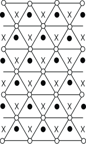
Figure 1: Comparison of the layers that form the hcp and fcc structures. Both of the structures have the empty circles (A) as one layer. However, the hcp lattice has a layer of the darkened circles (B) above and below that layer; whereas, the fcc lattice has a layer of the darkened circles (B) above and a layer of the X’s (C) below.

In order to extend this study to higher precision we used a growth or epidemic analysis to determine precise values of the critical thresholds of the hcp lattice, which were then compared to those of the fcc lattice. We also carried out an exact enumeration study, because we couldn’t find any such series expansions for the hcp and fcc lattices in literature; we could only find an exact enumeration study of a modified fcc lattice [8].

In the following sections, we report on the determination of the new values of $p_{c}$ for the hcp lattice and the details of the exact enumeration. The results are summarized and discussed in the conclusion section.

2 Percolation thresholds

Precise values of the thresholds for bond and site percolation on the hcp lattice were found using procedures similar to those outlined for site percolation in [5] and for bond percolation in [6]. A virtual lattice of $2048^{3}$ sites was simulated, using the block-data method first described in [9]. We distorted both lattices so that all sites fell on a simple cubic lattice. On these lattices, we grew individual clusters by a Leath-type algorithm which used the unit vectors shown in Table 1 for the hcp and fcc lattices. For the hcp lattice, the unit vectors in the plane will always be the same, but the unit vectors needed to check the nearest neighbors above or below a certain site depends on which level the site is located ($A$ or $B$). In Table 1, the unit vectors required to check the nearest neighbors in the plane and when going from layer $A$ to $B$ and from $B$ to $A$ are shown for the hcp lattice. The critical thresholds were identified using an epidemic scaling analysis. In order to determine the critical thresholds at the reported precision, about $2\times 10^{7}$ clusters were generated utilizing about $10^{13}$ random numbers, which required a few weeks worth of computer time on ten workstations.

Table 1: Unit vectors used to describe the neighbors in the fcc and hcp lattices.

Lattice Vectors fcc $(1,1,0)$, $(1,-1,0)$, $(-1,-1,0)$, $(-1,1,0)$, $(1,0,1)$, $(-1,0,1)$, $(1,0,-1)$, $(-1,0,-1)$,$(0,1,1)$, $(0,-1,1)$, $(0,1,-1)$, $(0,-1,-1)$ hcp (in the plane) $(1,0,0)$, $(1,1,0)$, $(0,1,0)$, $(-1,0,0)$, $(-1,-1,0)$, $(0,-1,0)$, (A to B) $(0,0,1)$, $(0,0,-1)$, $(0,-1,1)$, $(0,-1,-1)$, $(1,0,1)$, $(1,0,-1)$ (B to A) $(0,0,1)$, $(0,0,-1)$, $(-1,0,1)$, $(-1,0,-1)$, $(0,1,1)$, $(0,1,-1)$

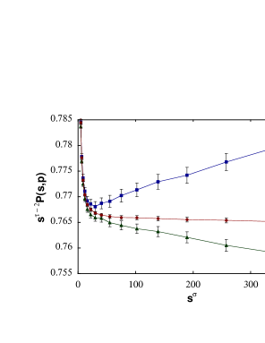
Figure 2: Plot of $s^{\tau-2}P(s,p)$ versus $s^{\sigma}$ for bond percolation on the hcp lattice. The curves plotted here represent $p=0.120\,170\,0$, $p=0.120\,163\,5$, and $p=0.120\,160\,0$ (from top to bottom) respectively.

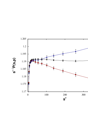
Figure 3: Plot of $s^{\tau-2}P(s,p)$ versus $s^{\sigma}$ for site percolation on the hcp lattice. The curves plotted here represent $p=0.199\,260\,0$, $p=0.199\,255\,5$, and $p=0.199\,250\,0$ (from top to bottom) respectively.

The simulation was used to find the fraction of clusters $P(s,p)$ that grew to a size greater than or equal to $s$ sites. When $p$ is near $p_{c}$, one expects $P(s,p)$ to behave as

$$P(s,p)\sim As^{2-\tau}f((p-p_{c})s^{\sigma})\approx As^{2-\tau}[1+C(p-p_{c})s^{\sigma}+\ldots]$$ (1)

where $\tau$ and $\sigma$ are universal exponents [1, 10]. We assumed the values $\tau=2.189$ and $\sigma=0.445$, which are consistent with other three-dimensional percolation studies [5, 6, 11, 12]. Plots of $s^{\tau-2}P(s,p)$ versus $s^{\sigma}$ for site and bond percolation on the hcp lattice were used to find the value of the percolation threshold which corresponds to horizontal behavior for large $s$. The results are plotted in Figures 2 and 3 and imply the following values for the critical thresholds for site (S) and bond (B) percolation:

$$p^{hcp}_{c,S}=0.199\,255\,5\pm 0.000\,001\,0$$

$$p^{hcp}_{c,B}=0.120\,164\,0\pm 0.000\,001\,0.$$ (2)

For the fcc lattice, we previously found the values [5, 6]:

$$p^{fcc}_{c,S}=0.199\,236\,5\pm 0.000\,001\,0$$

$$p^{fcc}_{c,B}=0.120\,163\,5\pm 0.000\,001\,0.$$ (3)

The site thresholds for these two lattices differ by only $0.000\,019$, which is statistically significant being nearly 10 combined error bars apart. The bond thresholds, on the other hand, are identical within the error bars.

3 Exact enumeration studies of the hcp and fcc lattices

The similarity of the thresholds for the hcp and fcc lattices led us to also carry out an exact enumeration calculation, to see how the series of the two lattices compare. In exact enumeration, the problem is to find $g_{st}$, the number of clusters containing $s$ occupied sites and $t$ vacant neighboring sites or bonds. Knowing $g_{st}$, one can find the number of clusters (per site) containing $s$ occupied sites by

$$n_{s}(p)=\sum_{t}g_{st}p^{s}q^{t}\ ,$$ (4)

the total number of clusters per site,

$$N=M_{0}(p)=\sum_{s}n_{s}=\sum_{s,t}g_{st}p^{s}q^{t}\ ,$$ (5)

the percolation probability,

$$P(q)=p-M_{1}(p)=p-\sum_{s}sn_{s}=p-\sum_{s,t}sg_{st}p^{s}q^{t}\ ,$$ (6)

(for small $q$), and the susceptibility,

$$S(p)=M_{2}(p)=\sum_{s}s^{2}n_{s}=\sum_{s,t}s^{2}g_{st}p^{s}q^{t}\ ,$$ (7)

where $q=1-p$. To calculate all these quantities, it is useful to construct the generating function

$$G(p,q)=\sum_{s,t}g_{st}p^{s}q^{t}\ .$$ (8)

To find $g_{st}$, we developed a rather simple enumeration method based upon the cluster-growth algorithm, but using a deterministic sequence to decide whether each successive site (or bond) is occupied or vacant. After a cluster was finished, we stepped back to the last vacant site and made it occupied (if $s$ was below the cutoff), or stepped back through the last group of occupied sites to first vacant one before it, and made that site occupied (if $s$ was at the cutoff), and then returned to the growth algorithm again. In this way we went through a binary search of all possible growth scenarios. This method is similar to the algorithm described by Redner [13]. We tested our algorithm with published results [14] in 2- and 3-dimensions, and found agreement. Although slower than Merten’s Fortran code [14], our program was easy to code and generalize for the different lattices and both site and bond percolation. We found the various series to $s=9$ in a few days of computer time.

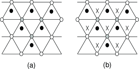
Figure 4: A triangular cluster of three sites (gray colored circles) on the (a) hcp and (b) fcc lattice. In (a), the empty circles represent vacant sites in the plane of the cluster, the black circles represent vacant sites above and below the plane. Neighboring this cluster, there are 9 perimeter sites in the plane, 6 perimeter sites in the plane above and 6 in the plane below, yielding $t=9+6+6=21$ total perimeter sites. In (b), the black circles represent the sites above the plane, and the X’s represent the sites below the plane. This lattice has 9 perimeter sites in the plane, 6 in the plane above, and 7 in the plane below, yielding $t=9+6+7=22$ total perimeter sites.

For bond percolation, we consider that $s$ represents the number of occupied sites in a cluster, irrespective of the number of bonds that are needed to connect them, and $t$ represents the number of vacant bonds. We thus define $g_{st}$ as the number of clusters containing $s$ occupied sites and $t$ vacant perimeter bonds. Note that no bond is placed in internal, redundant locations. A cluster containing $s$ occupied sites and $t$ vacant perimeter bonds has a weight $g_{st}p^{s-1}q^{t}$, because only $s-1$ occupied bonds are needed to connect the $s$ sites. Therefore, in bond percolation, all definitions (4)-(7) should actually be divided by $p$ on the right-hand-side, or equivalently those definitions actually give $pM_{n}(p)$.

First consider the $g_{st}$ itself, which we represent by the generating function (8), where the coefficients of $p^{s}$ are the perimeter polynomials. Up to order $s=5$, the results are:

$G^{fcc}_{S}=p{q}^{12}+6{p}^{2}{q}^{18}+{p}^{3}(8{q}^{22}+12{q}^{23}+30{q}^{24})+{p}^{4}(2{q}^{24}+27{q}^{26}+48{q}^{27}+96{q}^{28}+144{q}^{29}+158{q}^{30})$ $+{p}^{5}(24{q}^{28}+6{q}^{29}+132{q}^{30}+264{q}^{31}+423{q}^{32}$ $+780{q}^{33}+1194{q}^{34}+1212{q}^{35}+846{q}^{36})+\ldots$

$G^{hcp}_{S}=p{q}^{12}+6{p}^{2}{q}^{18}+{p}^{3}({q}^{21}+6{q}^{22}+13{q}^{23}+30{q}^{24})+{p}^{4}(8{q}^{25}+21{q}^{26}+48{q}^{27}+90{q}^{28}+150{q}^{29}+158{q}^{30})$ $+{p}^{5}({q}^{27}+12{q}^{28}+36{q}^{29}+114{q}^{30}+303{q}^{31}+357{q}^{32}+801{q}^{33}+1140{q}^{34}+1278{q}^{35}+840{q}^{36})+\ldots$

$G^{fcc}_{B}=p{q}^{12}+6{p}^{2}{q}^{22}+{p}^{3}(8{q}^{30}+16{q}^{31}+42{q}^{32})$ $+{p}^{4}(2{q}^{36}+6{q}^{37}+36{q}^{38}+84{q}^{39}+219{q}^{40}+249{q}^{41}+326{q}^{42})$ $+{p}^{5}(30{q}^{44}+120{q}^{45}+372{q}^{46}+792{q}^{47}+1596{q}^{48}+2328{q}^{49}+3576{q}^{50}+3072{q}^{51}+2739{q}^{52})+\ldots$

$G^{hcp}_{B}=pq^{12}+6p^{2}{q}^{22}+p^{3}(8{q}^{30}+16{q}^{31}+42{q}^{32})$ $+p^{4}(2{q}^{36}+6{q}^{37}+36{q}^{38}+84{q}^{39}+219{q}^{40}+249{q}^{41}+326{q}^{42})$ $+p^{5}({q}^{42}+4{q}^{43}+34{q}^{44}+114{q}^{45}+357{q}^{46}+780{q}^{47}+1611{q}^{48}+2382{q}^{49}+3513{q}^{50}+3090{q}^{51}+2739{q}^{52})+\ldots$

For site percolation, the differences between the two lattices start to show up with $s=3$. For example, the term for $s=3$ and $t=21$ occurs for the hcp but not the fcc lattice. This corresponds to the cluster of three sites in a triangle on the plane, as shown in Fig. 4.  For bond percolation, the first difference does not occur until $s=5$.

First we compare the moments for site percolation, writing each moment for the two different lattices adjacent to each other for easy comparison:

$$M_{0,S}^{fcc}=p-6p^{2}+8p^{3}+p^{4}-6p^{5}+30p^{6}-4p^{7}+105p^{8}+79p^{9}\dots$$

$$M_{0,S}^{hcp}=p-6p^{2}+8p^{3}+p^{4}-6p^{5}+30p^{6}+2p^{7}+33p^{8}+513p^{9}\dots$$

$$M_{1,S}^{fcc}/p=q^{12}+12q^{18}-12q^{19}+24q^{22}-12q^{23}+50q^{24}-168q^{25}+222q^{26}-140q^{27}+252q^{28}+\dots$$

$$M_{1,S}^{hcp}/p=q^{12}+12q^{18}-12q^{19}+3q^{21}+12q^{22}+6q^{23}+30q^{24}-109q^{25}+78q^{26}+41q^{27}+44q^{28}+\dots$$

$$M_{2,S}^{fcc}=p+12p^{2}+84p^{3}+504p^{4}+3012p^{5}+17142p^{6}+96228p^{7}+532028p^{8}+2918388p^{9}+\ldots$$

$$M_{2,S}^{hcp}=p+12p^{2}+84p^{3}+504p^{4}+3014p^{5}+17148p^{6}+96072p^{7}+533286p^{8}+2911166p^{9}+\ldots$$

For the first moment, we report $M_{1}/p$, which gives somewhat simpler expressions for the $q$ series than $M_{1}$. Note that the series are identical up to order $p^{6}$ for $M_{0}$, $q^{19}$ (three terms) for $M_{1}/p$, and $p^{4}$ for $M_{2}$. The coefficients for $M_{2}$ differ a small amount between the two lattices for higher order. Note that the series for $M_{1}(q)$ is actually given up to order 38 by the enumerations for $s\leq 9$.

For bond percolation, the corresponding series are:

$$pM_{0,B}^{fcc}=p-6{p}^{2}+8{p}^{4}+33{p}^{5}+132{p}^{6}+554{p}^{7}+2514{p}^{8}+13152{p}^{9}+\ldots$$

$$pM_{0,B}^{hcp}=p-6p^{2}+8p^{4}+33p^{5}+132p^{6}+553p^{7}+2526p^{8}+13116p^{9}+\dots$$

$M_{1,B}^{fcc}={q}^{12}+12{q}^{22}-12{q}^{23}+24{q}^{30}+54{q}^{32}-204{q}^{33}+126{q}^{34}+8{q}^{36}+96{q}^{38}-32{q}^{39}+276{q}^{40}-768{q}^{41}+608{q}^{42}-1800{q}^{43}+3066{q}^{44}-1304{q}^{45}+360{q}^{46}-480{q}^{47}+1056{q}^{48}-3360{q}^{49}+\ldots$

$M_{1,B}^{hcp}=q^{12}+12q^{22}-12q^{23}+24q^{30}+54q^{32}-204q^{33}+126q^{34}+8q^{36}+96q^{38}-32q^{39}+276q^{40}-768q^{41}+613q^{42}-1800q^{43}+3036q^{44}-1314q^{45}+450q^{46}-480q^{47}+1061q^{48}-3480q^{49}+\ldots$

$$pM_{2,B}^{fcc}=p+12{p}^{2}+132{p}^{3}+1356{p}^{4}+13344{p}^{5}+127548{p}^{6}+1194864{p}^{7}+11033256{p}^{8}+100692522{p}^{9}+\ldots$$

$$pM_{2,B}^{hcp}=p+12p^{2}+132p^{3}+1356p^{4}+13344p^{5}+127548p^{6}+1194944p^{7}+11033544p^{8}+100697070p^{9}+\ldots$$

Here we find an even closer agreement between the series of the two lattices than we found for site percolation. The series for both $pM_{0}$ and $pM_{2}$ agree between the two lattices up to order 6 and then differ by a very small amount for the three orders beyond that, while the series for $M_{1}$ agree up to order $q^{41}$ (first 12 terms). While it is impossible to prove or disprove that the thresholds for the fcc and hcp lattices are identical from these results, they clearly suggest that if the thresholds are indeed different, then they should be much closer for bond percolation than site percolation, as indeed we have found numerically.

4 Conclusions

As a result of this work, we have shown that the critical thresholds for site percolation on the two lattices are definitely different. The value of $p_{c}$ on the hcp lattice ($0.199\,255\,5\pm 0.000\,001\,0$) is nearly ten combined error bars away from the previously reported value [5] for the fcc lattice ($0.199\,236\,5\pm 0.000\,001\,0$). Also, the exact enumeration series for the two lattices begin to differ at relatively low order terms for site percolation.

On the other hand, even at high precision, the critical thresholds for bond percolation on the hcp and fcc lattices have the same value, within the error bars ($0.120\,164\,0\pm 0.000\,001\,0$). Although the series for bond percolation on the two lattices do differ, the difference is incredibly small and does not occur until higher order terms. While this difference does not rigorously rule out equaltiy of the thresholds, we guess that the thresholds are in fact slightly different, but by an amount too small to be seen in our numerical simulations.

References

[1] D. Stauffer and A. Aharony, An
Introduction to
Percolation Theory, Revised 2nd. Ed. (Taylor and Francis, London, 1994).
[2] M. Sahimi, Applications of Percolation Theory, (Taylor and Francis, London,
1992).
[3] Y. Y. Tarasevich and S. C. van der Marck, cond-mat/9906078.
[4] S. C. van der Marck, Phys. Rev. E 55, 1514 (1997); Erratum 56,
3732 (1997).
[5] C. D. Lorenz and R. M. Ziff, J. Phys. A 31, 8147, (1998).
[6] C. D. Lorenz and R. M. Ziff, Phys. Rev. E 57, 230
(1998).
[7] see, for example, C. Kittel, Introduction to Solid State Physics, 7th. Ed.
(John Wiley
& Sons, Inc., New York, 1996).
[8] J. L. Bocquet, Phys. Rev. B 50, 16386 (1994).
[9] R. M. Ziff, P. T. Cummings, and G. Stell,
J. Phys. A 17, 3009 (1984).
[10] M. E. Fisher, Ann. Phys., NY 3, 255 (1967).
[11] R. M. Ziff and G. Stell, University of Michigan Report No. 88-4, (1988).
[12] H. G. Ballesteros, L. A. Fernandez, V. Martin-Mayor, A. M. Sudupe, G. Parisi,
J. J. Ruiz-Lorenzo, J Phys. A 32, 1 (1999).