Interactions and Weak Localization: Perturbation Theory and Beyond

Abstract

We establish an explicit correspondence between perturbative and nonperturbative results in the problem of quantum decoherence in disordered conductors. We demonstrate that the dephasing time $\tau_{\varphi}$ cannot be unambiguously extracted from a perturbative calculation. We show that the effect of the electron-electron interaction on the magnetoconductance is described by the function $A_{d}(t)\exp(-f_{d}(t))$. The dephasing time is determined by $f_{d}(t)$, i.e. in order to evaluate $\tau_{\varphi}$ it is sufficient to perform a nonperturbative analysis with an exponential accuracy. The effect of interaction on the pre-exponent $A_{d}(t)$ is important if one calculates the interaction-dependent part of the weak localization correction for strong magnetic fields. The zero temperature dephasing time drops out of this correction in the first order due to the exact cancellation of the linear in time $T$-independent contributions from the exponent and the pre-exponent. Nonlinear in time $T$-independent contributions do not cancel out already in the first order of the perturbation theory and yield an additional contribution to dephasing at all temperatures including $T=0$.

I Introduction

Recent experiments by Mohanty, Jariwala and Webb [1] strongly indicate an intrinsic nature of a low temperature saturation of the electron decoherence time $\tau_{\varphi}$ in disordered conductors [2, 3]. It was argued in Refs. [1, 4] that zero point fluctuations of electrons could be responsible for a finite dephasing at low temperatures. These as well as various other recent experimental results attract a lot of attention to the fundamental role of interactions in disordered mesoscopic systems.

A theory of the above phenomenon [1] was proposed in our papers [5, 6]. We demonstrated that electron-electron interactions in disordered systems can indeed be responsible for a nonzero electron decoherence rate down to $T=0$. Our results [5, 6] are in a good agreement with experimental findings [1]. We also argued [7] that this interaction-induced decoherence has the same physical nature as in the case of a quantum particle interacting with a bath of harmonic oscillators [8, 9].

The low temperature saturation of the decoherence rate $1/\tau_{\varphi}$ on a level predicted in Refs. [5, 6] has serious theoretical consequences. Therefore it is not surprising that these predictions initiated intensive theoretical debates [10, 11, 12, 13, 14, 15, 16, 17, 18]. In contrast to Refs. [1, 4, 5, 6, 7], various authors [10, 11, 13, 15, 17, 18] argued that interaction-induced electron dephasing at $T\to 0$ is not possible. Vavilov and Ambegaokar (VA) [16] argued the quantum correction to the classical result [2, 3] should be small at least in the limit $T\tau_{\varphi}\gg 1$.

It should be emphasized that the above discussion goes far beyond the problem of electron dephasing only. This discussion is important for a general understanding of the role of the electron-electron interactions in mesoscopic systems at low temperatures. According e.g. to Aleiner, Altshuler and Gershenzon (AAG) [13] this role is merely to provide a (temperature dependent) renormalization of a disordered potential of impurities. Within this picture, at sufficiently low $T$ (when the effect of thermal fluctuations is small and can be neglected) electrons propagate in an effective inhomogeneous static potential which should be determined self-consistently in the presence of Coulomb interaction. If so, electron scattering on such a static potential is not any different from that on static impurities and, hence, cannot lead to dephasing. Our results [5, 6] suggest a different picture, according to which dynamical effects are important at all temperatures down to $T=0$ and the high frequency “quantum” modes with $\omega>T$ do contribute to dephasing.

Two main arguments supporting the first (“static”) picture are usually discussed [10, 11, 13, 15, 16, 17, 18]. The first argument is quite general and is not necessarily related to electrons in a disordered metal. One can argue [10, 13, 17] that a particle with energy $\sim T$ cannot excite harmonic oscillators with frequencies $\omega>T$ and, hence the latter will at most lead to renormalization effects. It is easy to observe, however, that this argument explicitly contradicts to the exact results obtained e.g. within the Caldeira-Leggett model [8]. There even at $T=0$ the off-diagonal elements of the particle density matrix decay at a finite length set by interaction. This effect is due to all high frequency modes of the effective environment, i.e. the picture is by no means “static” (see also Refs. [7, 12, 14] for further discussion).

One can also modify the above argument and conjecture [16] that the system of electrons can behave differently from a bosonic one [8] because of the Pauli principle which restricts scattering space for electrons at low $T$ and, hence, their ability to exchange energy. Again, this argument contradicts to the well known results obtained for fermionic systems. E.g. it is well established [19, 20] that tunneling electrons exchange energy with the effective environment (formed by other electrons in the leads) even at $T=0$. This exchange results in the temperature independent broadening of the effective energy distribution $P(E)$ for tunneling electrons [19]. This so-called “P(E)-theory” was verified in many experiments [21]. A close formal and physical similarity between the theory [19] and our analysis [6] is discussed in Ref. [22].

The second argument against the possibility of the interaction-induced saturation of $\tau_{\varphi}$ is purely formal. It is based on a perturbative calculation by AAG [13]. These authors claimed [11, 13] that the results of this calculation explicitly contradict to our results [5, 6] and, hence, the latter are incorrect. However, a convincing comparison between the two calculations was not presented. Furthermore, it our Reply [12, 14] we pointed out that the origin of the above controversy lies deeper, and the AAG’s suggestion that our calculation is “profoundly incorrect” can not be taken seriously. We argued that both approaches do agree on a perturbative level and the key difference between them is that our calculation [6] is nonperturbative while the analysis by AAG does not go beyond the first order in the interaction and, on top of that, involves additional approximations not contained in our paper [6]. For instance, for the exactly solvable Caldeira-Leggett model we demonstrated [12, 14] that within the perturbative approach involving analogous approximations one arrives at incorrect results and misses the effect of quantum decoherence at low temperatures.

Motivated by this discussion as well as by the fundamental importance of the problem we have undertaken an additional analysis of the effect of interaction-induced decoherence in disordered metals. This analysis will help us to demonstrate the actual relation between our approach [6] and that of AAG [13]. Since it is hardly possible to settle a calculational dispute without presenting sufficiently many details, in this paper we made an effort to provide the reader with such details of our calculation.

The structure of the paper is as follows. In section 2 we will demonstrate a principal insufficiency of the perturbation theory in the interaction for the problem of quantum dephasing. We will argue that $\tau_{\varphi}$ cannot be unambiguously extracted even from a correct perturbative calculation. In section 3 we extend our nonperturbative calculation [6]. We will carry out a complete analysis of the problem with the exponential accuracy. We will also present semi-quantitative arguments which, however, will be sufficient in order to understand the effect of interaction on the pre-exponent. In section 4 we perform a detailed perturbative calculation and demonstrate that at low $T$ some previous perturbative results are based on several insufficient approximations, the main of which is the golden rule approximation. We also establish an explicit relation between nonperturbative [6] and perturbative [13] calculations. A close formal similarity between the problem in question and the exactly solvable Caldeira-Leggett model is analyzed in section 5. In section 6 we briefly summarize our main observations. For the sake of convenience we will briefly announce the main steps of our calculation in the beginning of each section. Some further technical details are presented in Appendices A, B, C and D. In Appendix E we discuss the results [15, 16, 17].

II Insufficiency of the perturbation theory

In this section we will demonstrate a principal insufficiency of a perturbative (in the interaction) approach to the problem of quantum dephasing. In the subsection A we will present some general remarks concerning the role of the perturbation theory for the problem of a quantum mechanical particle interacting with other quantum degrees of freedom. In the subsection B we discuss the relation between perturbative and nonperturbative calculations of the magnetoconductance and the decoherence time $\tau_{\varphi}$ in disordered conductors.

A General remarks

The time evolution of the density matrix of such a particle is defined by the following equation:

$$\rho(t,x_{1f},x_{2f})=\int dx_{1i}dx_{2i}\;\;J(t,x_{1f},x_{2f},x_{1i},x_{2i})\rho(0,x_{1i},x_{2i}),$$ (1)

where $x$ is the particle coordinate. The kernel $J$ depends on the Feynman-Vernon influence functional [23, 24] and contains the full information about the effect of interaction. This kernel can formally be expanded in powers of the interaction strength

$$J(t)=\sum_{n=0}^{\infty}J^{(n)}(t).$$ (2)

The “noninteracting” kernel $J^{(0)}$ does not change the state of the system (provided its initial state is an eigenstate of the noninteracting Hamiltonian) and in this sense it is equivalent to the unity operator. All other terms of this expansion grow with time the faster the larger the number $n$ is. As a result in general all these terms (2) become important for sufficiently long times. Hence, the perturbation theory in the interaction (which amounts to keeping only several first terms of the expansion (2)) is equivalent to the short time expansion of the exact density matrix. Thus in general this perturbation theory cannot correctly describe the long time behavior of the interacting system no matter how weak the interaction is.

Keeping only the term $J^{(1)}$ in (2) under some additional assumptions one can express the probability $W_{ii}$ for the particle $x$ to remain in its initial state as

$$W_{ii}(t)=1-\int_{0}^{t}dt_{1}\int_{0}^{t_{1}}dt_{2}K(t_{1},t_{2}),$$ (3)

where the kernel $K(t_{1},t_{2})$ can be derived from the influence functional [24] and will not be specified here. In equilibrium one usually has $K(t_{1},t_{2})\equiv K(t_{1}-t_{2})$. Eq. (3) applies at short times, when the second term is still much smaller than unity. But even in this limit the correct information can be missed by insufficient approximations. For instance, the frequently used approximation amounts to retaining only the $\omega=0$ term in the kernel $K_{\omega}=\int(d\tau/2\pi)K(\tau)\exp(i\omega\tau)$. Within this so-called golden rule approximation one finds

$$W_{ii}(t)=1-\Gamma t,\;\;\;\;\;\;\Gamma=\pi K_{\omega=0}.$$ (4)

Furthermore, assuming that the effect of higher order terms in the expansion (2) can be accounted for by exponentiating the last term in (4) one immediately arrives at $W_{ii}(t)=\exp(-\Gamma t)$.

Obviously the above set of approximations is justified only in special cases. For instance, the golden rule approximation can work only provided the kernel $K(\tau)$ decays rapidly as compared to other relevant time scales in the problem. This could be the case e.g. at sufficiently high temperatures. In general, and especially in the low temperature limit, the golden rule approximation (4) fails. And it is particularly dangerous to combine the short time perturbative expansion with the long time golden rule approximation. E.g. if $K_{\omega=0}$ happens to be zero, it would follow from (4) that the particle will stay in its initial state forever even in the presence of interaction. Obviously this cannot be the case. The exponential decay of the probability $W_{ii}$ in time is also an artifact of the golden rule approximation. In general the time dynamics of an interacting system is much more complicated, and it should be determined from eq. (1).

In eq. (1) is usually implied that the initial density matrix $\rho(0)$ does not coincide with the exact reduced equilibrium density matrix for the interacting system. The standard approach is simply to factorize the initial density matrix [23, 24], i.e. to represent it as a product of the particle density matrix $\rho(0,x_{1i},x_{2i})$ and the equilibrium density matrix of all other degrees of freedom. In this case, even if initially both the particle and the environment were in their noninteracting ground states at $T=0$, the relaxation process occurs because the factorized density matrix does not describe the ground state of the interacting system. One could question the relevance of such initial conditions e.g. to the problem of electron transport in disordered conductors in the presence of interaction. Indeed, in this case the density matrix is never factorized and no time evolution can be expected for the equilibrium density matrix of the whole interacting system. Hence, at $T=0$ in equilibrium no relaxation should occur.

In order to clarify the situation let recall the formal expression for the conductivity (see the eq. (A36))

$$\sigma\propto\int\limits_{-\infty}^{t}dt^{\prime}\int d\mathchoice{{\hbox{\boldmath$\displaystyle r$}}}{{\hbox{\boldmath$\textstyle r$}}}{{\hbox{\boldmath$\scriptstyle r$}}}{{\hbox{\boldmath$\scriptscriptstyle r$}}}_{1i}d\mathchoice{{\hbox{\boldmath$\displaystyle r$}}}{{\hbox{\boldmath$\textstyle r$}}}{{\hbox{\boldmath$\scriptstyle r$}}}{{\hbox{\boldmath$\scriptscriptstyle r$}}}_{2i}J(t-t^{\prime},d\mathchoice{{\hbox{\boldmath$\displaystyle r$}}}{{\hbox{\boldmath$\textstyle r$}}}{{\hbox{\boldmath$\scriptstyle r$}}}{{\hbox{\boldmath$\scriptscriptstyle r$}}}_{1f},d\mathchoice{{\hbox{\boldmath$\displaystyle r$}}}{{\hbox{\boldmath$\textstyle r$}}}{{\hbox{\boldmath$\scriptstyle r$}}}{{\hbox{\boldmath$\scriptscriptstyle r$}}}_{2f},d\mathchoice{{\hbox{\boldmath$\displaystyle r$}}}{{\hbox{\boldmath$\textstyle r$}}}{{\hbox{\boldmath$\scriptstyle r$}}}{{\hbox{\boldmath$\scriptscriptstyle r$}}}_{1i},d\mathchoice{{\hbox{\boldmath$\displaystyle r$}}}{{\hbox{\boldmath$\textstyle r$}}}{{\hbox{\boldmath$\scriptstyle r$}}}{{\hbox{\boldmath$\scriptscriptstyle r$}}}_{2i})\rho_{\rm eff}(\mathchoice{{\hbox{\boldmath$\displaystyle r$}}}{{\hbox{\boldmath$\textstyle r$}}}{{\hbox{\boldmath$\scriptstyle r$}}}{{\hbox{\boldmath$\scriptscriptstyle r$}}}_{1i},\mathchoice{{\hbox{\boldmath$\displaystyle r$}}}{{\hbox{\boldmath$\textstyle r$}}}{{\hbox{\boldmath$\scriptstyle r$}}}{{\hbox{\boldmath$\scriptscriptstyle r$}}}_{2i}),$$ (5)

where $\rho_{\rm eff}(\mathchoice{{\hbox{\boldmath$\displaystyle r$}}}{{\hbox{\boldmath$\textstyle r$}}}{{\hbox{\boldmath$\scriptstyle r$}}}{{\hbox{\boldmath$\scriptscriptstyle r$}}}_{1i},\mathchoice{{\hbox{\boldmath$\displaystyle r$}}}{{\hbox{\boldmath$\textstyle r$}}}{{\hbox{\boldmath$\scriptstyle r$}}}{{\hbox{\boldmath$\scriptscriptstyle r$}}}_{2i})=(\mathchoice{{\hbox{\boldmath$\displaystyle r$}}}{{\hbox{\boldmath$\textstyle r$}}}{{\hbox{\boldmath$\scriptstyle r$}}}{{\hbox{\boldmath$\scriptscriptstyle r$}}}_{1i}-\mathchoice{{\hbox{\boldmath$\displaystyle r$}}}{{\hbox{\boldmath$\textstyle r$}}}{{\hbox{\boldmath$\scriptstyle r$}}}{{\hbox{\boldmath$\scriptscriptstyle r$}}}_{2i})\rho_{0}(\mathchoice{{\hbox{\boldmath$\displaystyle r$}}}{{\hbox{\boldmath$\textstyle r$}}}{{\hbox{\boldmath$\scriptstyle r$}}}{{\hbox{\boldmath$\scriptscriptstyle r$}}}_{1i},\mathchoice{{\hbox{\boldmath$\displaystyle r$}}}{{\hbox{\boldmath$\textstyle r$}}}{{\hbox{\boldmath$\scriptstyle r$}}}{{\hbox{\boldmath$\scriptscriptstyle r$}}}_{2i})$ and $\rho_{0}$ is the equilibrium electron density matrix. We observe that the effective initial density matrix $\rho_{\rm eff}$ in this expression is strongly perturbed at all $T$ as compared to $\rho_{0}$ due to the factor $(\mathchoice{{\hbox{\boldmath$\displaystyle r$}}}{{\hbox{\boldmath$\textstyle r$}}}{{\hbox{\boldmath$\scriptstyle r$}}}{{\hbox{\boldmath$\scriptscriptstyle r$}}}_{1i}-\mathchoice{{\hbox{\boldmath$\displaystyle r$}}}{{\hbox{\boldmath$\textstyle r$}}}{{\hbox{\boldmath$\scriptstyle r$}}}{{\hbox{\boldmath$\scriptscriptstyle r$}}}_{2i})$. Therefore relaxation always takes place in our problem. Since for a dissipative system relaxation times do not depend on the initial conditions, one can safely assume the initial density matrix to be, for instance, factorized. Actually the same assumption is used within the diagrammatic approach: a complete equivalence between eq. (A36) (factorized density matrix) and the diagrammatic expression for the conductance [13] was demonstrated in Appendix A in the first order in the interaction.

B Magnetoconductance

The weak localization correction to the conductivity of a disordered metal can be expressed in the following form

$$\delta\sigma_{d}(H)=-\frac{2e^{2}D}{\pi}\int\limits_{\tau_{e}}^{\infty}dtA_{d}(t)\exp\left(-t/\tau_{H}-f_{d}(t)\right),$$ (6)

$\tau_{e}=l/v_{F}$ is the elastic electron mean free time. The function $f_{d}(t)$ increases with time and describes the Cooperon decay due to interaction ($f_{d}(t)$ equals to zero without interaction). The presence of the magnetic field $H$ causes an additional decay on a time scale $\sim\tau_{H}$. By varying the magnetic field and thus $\tau_{H}$ (which decreases with increasing $H$) one can extract information about the interaction-induced decoherence directly from the magnetoconductance measurements.

The pre-exponential function $A_{d}(t)$ without interaction is $A_{d}^{(0)}(t)=1/(4\pi Dt)^{d/2}$. In the presence of interaction the function $A_{d}(t)$ will, of course, depend on the interaction as well. As it is demonstrated below, this dependence is can be ignored while calculating the decoherence time $\tau_{\varphi}$ which should only be extracted from the function $f_{d}(t)$ in the exponent of (6). This is the procedure of Ref. [6]. However, the dependence of the pre-exponent $A_{d}(t)$ on the interaction is important if one wants to recover the subleading in $\tau_{H}/\tau_{\varphi}$ term in the expression for $\delta\sigma_{d}(H)$ in the limit of a strong magnetic field $\tau_{H}\ll\tau_{\varphi}$. In this case only short times $t\lesssim\tau_{H}$ contribute to the integral (6) and it is sufficient to perform a short time expansion of both $\exp(-f_{d}(t))$ and $A_{d}(t)$. This expansion mixes terms important and unimportant for dephasing and in general makes it impossible to extract correct information about the dephasing time $\tau_{\varphi}$ from the perturbation theory even in the limit of strong magnetic fields $\tau_{H}\ll\tau_{\varphi}$.

In order to illustrate this conclusion let us restrict ourselves to a quasi-1d case. The expression (6) may then be rewritten as follows

$$\delta\sigma_{1}(H)=-\frac{e^{2}\sqrt{D}}{\pi^{3/2}}\int\limits_{0}^{+\infty}\frac{dt}{\sqrt{t}}e^{-t/\tau_{H}}F(t/\tau_{\varphi}),$$ (7)

where the function $F(t/\tau_{\varphi})$ accounts for the interaction. Note, that the function $F$ can (and in general does) depend not only on one but on several parameters $F=F(t/\tau_{1},t/\tau_{2},...,t/\tau_{n})$. In this section we will assume that $F$ depends on only one parameter $\tau_{\varphi}$. This is sufficient for our purposes.

In the absence of interaction $F\equiv 1$ and the divergence in the integral (7) is cut at times $t\sim\tau_{H}$. In this case from (7) we reproduce the well known result

$$\delta\sigma^{(0)}_{1}=-\frac{e^{2}}{\pi}\sqrt{D\tau_{H}}.$$ (8)

For large $\tau_{H}$ (i.e. for $H\to 0$) the result (8) diverges and the effect of interaction should be taken into account. Provided in the long time limit the function $F$ decays faster than $1/\sqrt{t}$ the integral (7) converges even for $1/\tau_{H}=0$ and we get

$$\delta\sigma_{1}=-a\frac{e^{2}}{\pi}\sqrt{D\tau_{\varphi}},$$ (9)

where the prefactor $a\sim 1$ which depends on the function $F$. The precise definition of $a$ is of little practical interest since this prefactor can always be removed by rescaling of $\tau_{\varphi}$. Of importance, however, is to describe the behavior of the function $F(t/\tau_{\varphi})$ at $t\sim\tau_{\varphi}$. This allows to determine the magnitude of the dephasing time $\tau_{\varphi}$. Clearly, a nonperturbative analysis in the interaction is needed in order to determine the function $F$ at times $t\sim\tau_{\varphi}$ simply because there exists no small parameter in the problem. E.g. if one would formally decrease the interaction strength, the magnitude of the dephasing time $\tau_{\varphi}$ would increase, but one would never avoid the necessity to determine the function $F$ at $t\sim\tau_{\varphi}$. Thus the problem of finding the decoherence time in disordered conductors is nonperturbative for any interaction strength. In this respect the statement of Ref. [17] that “since $\tau_{\varphi}$ is much longer than the elastic scattering time, the dephasing is weak and there is no need to invoke nonperturbative ideas” remains puzzling to us. Indeed, at times of order $\tau_{\varphi}$ the dephasing is strong by definition, and it is not clear how the condition $\tau_{\varphi}\gg\tau_{e}$ might help to avoid “nonperturbative ideas”.

Observing this problem AAG [13] suggested to consider the limit of strong magnetic fields $\tau_{H}\ll\tau_{\varphi}$, for which the integral (7) converges already at times $t\sim\tau_{H}$ much shorter than $\tau_{\varphi}$. In this case the weak localization correction can be calculated perturbatively in the interaction or, equivalently, by means a short time expansion of the function $F$. The recipe to evaluate the dephasing time from the perturbation theory suggested by AAG can be summarized as follows.

In the zero order in the interaction we have $F=1$ and the magnitude of the weak localization correction (8) increases as $\sqrt{\tau_{H}}$ with increasing $\tau_{H}$. If, expanding in the interaction, one would recover the term $\propto\sqrt{\tau_{H}}$, this term could just be added to (8) and interpreted as an interaction-induced renormalization effect of the bare parameters. The presence of such a term would imply that $F$ is not anymore equal to one but acquires some interaction correction. Nevertheless no time dependence of $F$ and, hence, no dephasing occurs in this case and therefore the terms $\propto\sqrt{\tau_{H}}$ are not “dangerous”. If, however, the first order conductance correction is found to increase with $\tau_{H}$ faster than $\sqrt{\tau_{H}}$ and to have an opposite with respect to $\delta\sigma^{(0)}_{1}$ (8) (i.e. positive) sign, this would already mean that the function $F$ depends on time (decays with increasing $t$) due to interaction and, hence, nonzero dephasing occurs. Then, if such “dephasing” terms are recovered within this perturbative procedure, one should look at a temperature dependence of such terms. If these terms are present at a finite $T$, but decrease and vanish as temperature approaches zero this would imply that interaction does not cause any dephasing at $T=0$. If $T$-independent positive terms growing faster than $\sqrt{\tau_{H}}$ are recovered one would be able to conclude that nonzero dephasing occurs at $T=0$ already within the first order perturbation theory in the interaction.

We are going to demonstrate that the above perturbative strategy in principle cannot be used to correctly obtain the dephasing time $\tau_{\varphi}$ for any magnetic field even though the correction $\delta\sigma_{H}$ can be evaluated perturbatively in the limit $\tau_{H}\ll\tau_{\varphi}$.

To begin with, we note that already the terms $\propto\sqrt{\tau_{H}}$ can easily cause troubles provided they give a (positive) contribution to $\delta\sigma_{1}(H)$ large as compared to the magnitude of the zero order term (8). In fact, the presence of terms $\propto\sqrt{\tau_{H}}$ just implies that their time dependence saturates already at short times $t\lesssim\tau_{H}$. If this saturated value turns out to exceed the zero order term, this would only indicate the breakdown of the perturbation expansion in the interaction and, hence, no definite conclusion from this expansion can be drawn.

An even much more important problem is that the form of the function $F(t)$ in (7) cannot be recovered from the perturbation theory at all. It is quite obvious that the first order perturbative terms will depend only on the derivative $F^{\prime}(0)$. Although in the limit $\tau_{H}\ll\tau_{\varphi}$ the value $\delta\sigma_{1}(H)$ can be calculated perturbatively in the interaction, this would yield no information about the dephasing time $\tau_{\varphi}$. Such information can be extracted only if one assumes some particular form of the function $F(t/\tau_{\varphi})$. But this form should be found rather than assumed. This task can be accomplished only if one goes beyond the perturbation theory.

Let us consider several different functions $F(t/\tau_{\varphi})$. Perhaps the most frequent choice of this function is based on the assumption about purely exponential decay of the phase correlations, in which case one has

$$F(t/\tau_{\varphi})=\exp(-t/\tau_{\varphi}).$$ (10)

As it was already discussed above, this form of the function $F$ follows directly from the golden rule approximation. Substituting (10) into (7) in the limit of weak magnetic fields $\tau_{H}\gg\tau_{\varphi}$ one immediately arrives at the result for the weak localization correction of the form (8) with $\tau_{H}$ substituted by $(1/\tau_{H}+1/\tau_{\varphi})^{-1}$. In the limit of weak magnetic fields $\tau_{H}\gg\tau_{\varphi}$ the result (9) with $a=1$ is recovered. In the opposite limit $\tau_{H}\ll\tau_{\varphi}$ eqs. (7) and (10) yield

$$\delta\sigma_{1}-\delta\sigma^{(0)}_{1}\simeq\frac{e^{2}}{2\pi}\frac{\sqrt{D}\tau_{H}^{3/2}}{\tau_{\varphi}},$$ (11)

where $\delta\sigma^{(0)}_{1}$ is defined in (8). Another possible choice of the function $F$ can be

$$F(t/\tau_{\varphi})=\exp(-(t/\tau_{\varphi})^{3/2}).$$ (12)

The reason for such a choice will become clear later. The substitution of (12) into (7) again yields the result (9) (with $a=2\Gamma(1/3)/3\sqrt{\pi}\simeq 1.0076$, $\Gamma(x)$ is the Euler gamma-function) in the limit $\tau_{H}\gg\tau_{\varphi}$, while in the opposite limit $\tau_{H}\ll\tau_{\varphi}$ from (7) and (12) one obtains

$$\delta\sigma_{1}-\delta\sigma^{(0)}_{1}\simeq\frac{e^{2}\sqrt{D\tau_{H}}}{\pi^{3/2}}\left(\frac{\tau_{H}}{\tau_{\varphi}}\right)^{3/2}.$$ (13)

Comparing (11) and (13) we observe that for strong magnetic fields the interaction corrections to the leading order term (8) are different depending on the choice of the function $F$, even though for weak magnetic fields both choices (10) and (12) yield the same result (9) with only slightly different values of a numerical prefactor $a$.

The magnetoresistance data are frequently fitted to the formula [3]

$$\delta\sigma_{1}(H)=\frac{e^{2}}{\pi}\sqrt{D\tau_{\varphi}}\frac{{\rm Ai}(\tau_{\varphi}/\tau_{H})}{{\rm Ai}^{\prime}(\tau_{\varphi}/\tau_{H})},$$ (14)

where Ai$(x)$ is the Airy function. In the limit $\tau_{H}\gg\tau_{\varphi}$ this equation again reduces to (9) with the factor $a=-{\rm Ai}(0)/{\rm Ai}^{\prime}(0)\simeq 1.372$. In the opposite limit $\tau_{H}\ll\tau_{\varphi}$ one finds

$$\delta\sigma_{1}-\delta\sigma_{1}^{(0)}\simeq\frac{e^{2}\sqrt{D\tau_{H}}}{4\pi}\left(\frac{\tau_{H}}{\tau_{\varphi}}\right)^{3/2}.$$ (15)

We observe the equivalence between (13) and (15) up to a numerical prefactor of order one.

Finally, let choose the trial function $F$ in the following form:

$$F(t/\tau_{\varphi})=\frac{e^{-t/\tau_{\varphi}}\sqrt{bt}}{\sqrt{\tau_{\varphi}(1-e^{-bt/\tau_{\varphi}})}},$$ (16)

where $b$ is a numerical coefficient of order one. Combining (7) and (16) we find

$$\delta\sigma_{1}(H)=-\frac{e^{2}}{\pi}\sqrt{D\tau_{\varphi}}\frac{1}{\sqrt{b}}\frac{\Gamma\left(\frac{1}{b}\left(1+\frac{\tau_{\varphi}}{\tau_{H}}\right)\right)}{\Gamma\left(\frac{1}{2}+\frac{1}{b}\left(1+\frac{\tau_{\varphi}}{\tau_{H}}\right)\right)}.$$ (17)

In the limit $\tau_{H}\ll\tau_{\varphi}$ one can expand this equation in powers of $\tau_{H}/\tau_{\varphi}$ and get

$$\delta\sigma_{1}-\delta\sigma^{(0)}_{1}\simeq\frac{4-b}{4}\frac{e^{2}\sqrt{D\tau_{H}}}{2\pi}\frac{\tau_{H}}{\tau_{\varphi}},$$ (18)

while in the limit $\tau_{H}\gg\tau_{\varphi}$ from (7), (16) one again recovers eq. (9) with a slightly modified numerical prefactor $a$ (which now also depends on the value $b$). Absorbing $a$ by a proper redefinition of $\tau_{\varphi}$ one can plot the result (7) for the trial functions (10), (16) (for different values of $b$) and eq. (14) depending on the magnetic field (or $\tau_{H}$). These plots are presented in Fig. 1. We observe that all four plotted functions are very close to each other (e.g. the maximum deviation between (14) and $\delta\sigma_{1}(H)$ obtained from (16) with $b=4$ does not exceed 0.01). If one would fit the experimental data for the magnetoconductance with any of these four functions one (i) would not be able to distinguish between them within typical error bars and (ii) would obtain the same value $\tau_{\varphi}$ for all these functions (up to a prefactor $a\sim 1$ absorbed in $\tau_{\varphi}$ anyway). In other words, the results for $\tau_{\varphi}$ extracted from fitting the experimental data to several different functions $F(t/\tau_{\varphi})$ will be practically insensitive to the particular form of $F$ as long as its decay at long times is sufficiently fast to provide an effective cutoff for the integral (7) at $t\sim\tau_{\varphi}$.

At the same time if one tries to extract $\tau_{\varphi}$ from the perturbation theory in the interaction one immediately arrives at ambiguous and contradictory results. Let us, for example, consider the perturbative result of AAG

$$\delta\sigma_{1}-\delta\sigma^{(0)}_{1}\propto T\tau_{H}^{2}$$ (19)

(see e.g. eq. (4.8b) of Ref. [13]) and, following the above paper, assume an exponential decay of correlations (10). In this case the dephasing time $\tau_{\varphi}$ is obtained from a direct comparison of eq. (11) (equivalent to eq. (4.3b) of Ref. [13] or eq. (3) of Ref. [11]) with eq. (19) (or eq. (4.8b) in Ref. [13]). One obtains

$$1/\tau_{\varphi}^{AAG}\propto T\sqrt{\tau_{H}}$$ (20)

(cf. eq. (4.9b) of Ref. [13]). The result (20) is essentially based on the assumption about a purely exponential decay (10). Note, however, that a-priori there is no reason to assume such a decay. [Just on the contrary, it will be demonstrated below that this is not the case for the problem in question.] The cutoff functions (12), (16) (and many others) yield the same result (9) as the function (10) and one can hardly make a distinction between them from the magnetoconductance measurements (Fig. 1).

For instance, if one sticks to the choice (12), one should extract $\tau_{\varphi}$ by comparing eqs. (13) and (19). This comparison yields $\tau_{\varphi}$ independent of $\tau_{H}$ and $1/\tau_{\varphi}\propto T^{2/3}$. The latter form coincides with the well known result by Altshuler, Aronov and Khmelnitskii (AAK) [2] but is in an obvious disagreement with (20). If, instead of (12), one uses the trial function (16) and compares (18) and (20), one finds $\tau_{\varphi}\propto(4-b)/(T\tau_{H}^{1/2})$, i.e. positive, zero and even negative (!) dephasing times respectively for $b<4$, $b=4$ and $b>4$. However, all these dramatic differences in the first order results have no effect both on the form of the magnetoconductance $\delta\sigma_{d}(H)$ (Fig. 1) and on the value $\tau_{\varphi}$ extracted from it.

Thus, whatever result is obtained in the first order perturbation theory in the interaction, it is yet insufficient to draw any definite conclusion about the dephasing time $\tau_{\varphi}$. The problem is essentially nonperturbative and should be treated as such. The corresponding analysis was developed in our paper [6] and will be extended further in the next section.

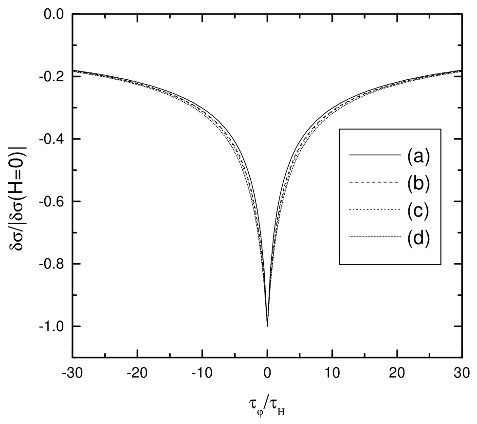
FIG. 1.: Magnetoconductance curves corresponding to different cutoff procedures: (a) purely exponential cutoff (10); (b) Airy function of eq. (14)); (c) the cutoff function $F$ is given by the eq. (16) with $b=4$ ($a\simeq 1.479$) corresponding to “zero dephasing” in the first order perturbation theory; (d) the cutoff function (16) with $b=5$ ($a\simeq 1.582$) which yields “negative dephasing” in the first order perturbation theory. Here $\tau_{\varphi}$ is rescaled to absorb the factor $a$ in eq. (9).

III Weak Localization Correction: Nonperturbative Results

In order to provide a complete description of the electron-electron interaction effect on the weak localization correction (6) it is in general necessary to calculate both the function $f_{d}(t)$ in the exponent of (6) and the pre-exponential function $A_{d}(t)$. An important observation is, however, that information about the effect of interaction on $A_{d}(t)$ is not needed to correctly evaluate the dephasing time $\tau_{\varphi}$. It suffices to find only the function $f_{d}(t)$ which describes the decay of correlations in time and provides an effective cutoff for the integral (6) at $t\sim\tau_{\varphi}$. The role of the pre-exponent is merely to establish an exact numerical prefactor. Since $\tau_{\varphi}$ is defined up to a numerical prefactor of order one anyway, it is clear that only the function $f_{d}(t)$ – and not $A_{d}(t)$ – is really important.

In the subsection A we extend our previous analysis [6] and evaluate of the function $f_{d}(t)$ keeping all the subleading terms. This procedure is important in at least two aspects: (i) it allows to unambiguously settle the issue of unphysical divergences which was argued by VA [16] to be a problem in our previous calculation [6] and (ii) it is necessary to establish a direct relation between our nonperturbative approach and the perturbation theory in the interaction. In the subsection B we will perform a semi-quantitative analysis of the effect of interactions on the pre-exponential function $A_{d}(t)$. In the subsection C we will demonstrate that the short time perturbative expansion of both the exponent and the pre-exponent at low $T$ not only can (section 2B) but does lead to missing an important information about $\tau_{\varphi}$ in disordered conductors.

A Exponent

The function $f_{d}(t)$ can be evaluated by means of the path integral formalism [6]. This procedure amounts to calculating the path integral for the kernel of the evolution operator

$$J\sim\int{\cal D}\mathchoice{{\hbox{\boldmath$\displaystyle r$}}}{{\hbox{\boldmath$\textstyle r$}}}{{\hbox{\boldmath$\scriptstyle r$}}}{{\hbox{\boldmath$\scriptscriptstyle r$}}}\int{\cal D}\mathchoice{{\hbox{\boldmath$\displaystyle p$}}}{{\hbox{\boldmath$\textstyle p$}}}{{\hbox{\boldmath$\scriptstyle p$}}}{{\hbox{\boldmath$\scriptscriptstyle p$}}}\,\exp(iS_{0}-iS_{0}^{\prime}-iS_{R}-S_{I})$$ (21)

within the saddle point approximation on pairs of time reversed paths and to averaging over diffusive trajectories. Here $S_{0}$ and $S_{0}^{\prime}$ represent the electron action on the two parts of the Keldysh contour, while $iS_{R}+S_{I}$ accounts for the interaction. The effective action (21) was derived in our Ref. [6], for the sake of convenience we reproduce the explicit expressions in Appendix A (eqs. (A38-A45)) together with the expression for the conductance of a disordered metal in terms of the kernel of the evolution operator $J$ and the electron density matrix (A36).

The saddle point approximation procedure was described in details in Ref. [6]. One can demonstrate that the contribution of the real part $S_{R}$ of the action (A43) vanishes on any pair of time reversed diffusive paths. By no means this cancellation occurs by chance, rather it is a generic property of a wide class of influence functionals describing dissipative environments. E.g. similar cancellation is observed in the Caldeira-Leggett model [8], the relation to which will be discussed in Section 5. Also we would like to point out that for any pair of paths $S_{R}$ contributes only to the real part of the effective action and, hence, can never cancel an imaginary contribution from the term $S_{I}$ (A45). Anyway, the function $f_{d}(t)$ in the exponent is determined solely by the imaginary part of the action $S_{I}$ (A45) and it is given by the following expression [6]:

$$f_{d}(t)=e^{2}\int\limits_{0}^{t}dt_{1}\int\limits_{0}^{t}dt_{2}\left\langle I(t_{1}-t_{2},\mathchoice{{\hbox{\boldmath$\displaystyle r$}}}{{\hbox{\boldmath$\textstyle r$}}}{{\hbox{\boldmath$\scriptstyle r$}}}{{\hbox{\boldmath$\scriptscriptstyle r$}}}(t_{1})-\mathchoice{{\hbox{\boldmath$\displaystyle r$}}}{{\hbox{\boldmath$\textstyle r$}}}{{\hbox{\boldmath$\scriptstyle r$}}}{{\hbox{\boldmath$\scriptscriptstyle r$}}}(t_{2}))-I(t_{1}+t_{2}-t,\mathchoice{{\hbox{\boldmath$\displaystyle r$}}}{{\hbox{\boldmath$\textstyle r$}}}{{\hbox{\boldmath$\scriptstyle r$}}}{{\hbox{\boldmath$\scriptscriptstyle r$}}}(t_{1})-\mathchoice{{\hbox{\boldmath$\displaystyle r$}}}{{\hbox{\boldmath$\textstyle r$}}}{{\hbox{\boldmath$\scriptstyle r$}}}{{\hbox{\boldmath$\scriptscriptstyle r$}}}(t_{2}))\right\rangle_{\rm diff},$$ (22)

where the function $I$ is defined in (A35). In equilibrium it is expressed in terms of an imaginary part of the inverse effective dielectric susceptibility $1/\epsilon(\omega,k)$ multiplied by $\coth(\omega/2T)$. The first term (22) describes the contribution of the self energy diagrams (diagrams (a) and (b) in Fig. 2), while the second term is due to the vertex diagrams ((c) and (d) in Fig. 2). In order to evaluate the function $f_{d}(t)$ (22) we introduce the Fourier transform of the function $I$ and then average over the diffusive trajectories with the aid of a standard replacement [25] $\langle\exp[i\mathchoice{{\hbox{\boldmath$\displaystyle k$}}}{{\hbox{\boldmath$\textstyle k$}}}{{\hbox{\boldmath$\scriptstyle k$}}}{{\hbox{\boldmath$\scriptscriptstyle k$}}}(\mathchoice{{\hbox{\boldmath$\displaystyle r$}}}{{\hbox{\boldmath$\textstyle r$}}}{{\hbox{\boldmath$\scriptstyle r$}}}{{\hbox{\boldmath$\scriptscriptstyle r$}}}(t_{1})-\mathchoice{{\hbox{\boldmath$\displaystyle r$}}}{{\hbox{\boldmath$\textstyle r$}}}{{\hbox{\boldmath$\scriptstyle r$}}}{{\hbox{\boldmath$\scriptscriptstyle r$}}}(t_{2}))]\rangle_{\rm diff}=\exp(-Dk^{2}|t_{1}-t_{2}|)$. After the integration over $\textstyle k$ we obtain

$$f_{d}(t) = \frac{4e^{2}D^{1-d/2}}{\sigma_{d}(2\pi)^{d}}\left(\int\frac{d^{d}x}{1+x^{4}}\right)\int\frac{d\omega\;d\omega^{\prime}}{(2\pi)^{2}}\left[|\omega^{\prime}|^{d/2-2}(\omega-\omega^{\prime})\coth\frac{\omega-\omega^{\prime}}{2T}\;\frac{1-\cos\omega t}{\omega^{2}}\right.$$ (24)

$$\left.-|\omega^{\prime}|^{d/2-2}\omega\coth\frac{\omega}{2T}\;\frac{\cos\omega t-\cos\omega^{\prime}t}{\omega^{\prime 2}-\omega^{2}}\right].$$

Here again the first and the second terms in the square brackets are respectively from the self energy (Fig. 2a,b) and the vertex (Fig. 2c,d) diagrams. For 1d and 2d cases the integral of the first term over $\omega^{\prime}$ diverges at $\omega^{\prime}\to 0$. However, it is easy to check that this divergence is exactly canceled by the second term, the whole integral is finite in any dimension and does not require artificial infrared cutoffs. Various divergences are rather inherent to the perturbation theory in the interaction and – at least in part – are due to insufficiency of the perturbative expansion in our problem, especially at low temperatures. It is also useful to note that at $T\to 0$ the leading contribution to $f_{d}(t)$ in the long time limit is insensitive to a divergence contained in the first term in the square brackets (24) and can be derived only from this term [6].

The integrals in (24) can be handled in a straightforward manner. Technically it is sometimes more convenient to perform calculations in the real time rather than in the frequency representation. Here we will present the calculation for the 1d case.

First we find the explicit expression for $I(t,x)$ (A35):

$$I(t,x)=\frac{1}{\sigma_{1}}\int\frac{d\omega dk}{(2\pi)^{2}}\;\;\frac{\omega}{k^{2}}\coth\frac{\omega}{2T}\;\;e^{-i\omega t+ikx}=\frac{|x|}{2\pi\sigma_{1}}\left(-\frac{d}{dt}{\cal P}[\pi T\coth(\pi Tt)]\right).$$ (25)

Here ${\cal P}$ stands for the principal value, i.e. ${\cal P}[\pi T\coth(\pi Tt)]$ is a distribution rather than an ordinary function divergent at $t\to 0$. For a given diffusive trajectory (and on sufficiently long time scales) this function can be replaced by the following function of time

$$\langle I(t-0,x(t)-x(0))\rangle_{\rm diff} = \int dx\;I(t,x){\cal D}(|t|,x)=\frac{1}{2\pi\sigma_{1}}\left(-\frac{d}{dt}{\cal P}[\pi T\coth(\pi Tt)]\right)\int dx\;\frac{|x|\exp\left[-\frac{x^{2}}{4D|t|}\right]}{\sqrt{4\pi D|t|}}$$ (26)

$$= \frac{1}{\pi\sigma_{1}}\sqrt{\frac{D|t|}{\pi}}\left(-\frac{d}{dt}{\cal P}[\pi T\coth(\pi Tt)]\right).$$ (27)

Substitution of this equation in eq.(22) yields

$$f_{1}(t)=\frac{2e^{2}}{\pi\sigma_{1}}\int\limits_{0}^{t}dt_{1}\int\limits_{0}^{t_{1}}dt_{2}\left(-\frac{d}{dt}{\cal P}[\pi T\coth(\pi Tt)]\right)\left[\sqrt{\frac{Dt_{2}}{\pi}}-\sqrt{\frac{D|2t_{1}-t_{2}-t|}{\pi}}\right].$$ (28)

Let us first integrate this expression over $t_{1}$ and then integrate the result by parts. We obtain

$$f_{1}(t)=\frac{2e^{2}}{\pi\sigma_{1}}\sqrt{\frac{D}{\pi}}\int\limits_{2\tau_{e}/\pi}^{t}dt^{\prime}\;\pi T\coth(\pi Tt^{\prime})\left(\frac{t}{2\sqrt{t^{\prime}}}-\frac{3}{2}\sqrt{t^{\prime}}+\sqrt{t-t^{\prime}}\right).$$ (29)

The short time cutoff in (29) is equivalent to a sharp cutoff at $\omega=1/\tau_{e}$ in the frequency domain.

In the quantum regime $\pi Tt\ll 1$ we find

$$f_{1}(t)=\frac{e^{2}}{\pi\sigma_{1}}\sqrt{\frac{2D}{\tau_{e}}}t+\frac{2e^{2}}{\pi\sigma_{1}}\sqrt{\frac{Dt}{\pi}}\left(\ln\frac{2\pi t}{\tau_{e}}-6\right),\;\;\;\pi Tt\ll 1.$$ (30)

Note, that apart from the leading linear in time term there exists a a smaller term $\propto\sqrt{t}\ln(t/\tau_{e})$, which also grows in time.

In order to find the function $f_{1}(t)$ in the opposite thermal limit $\pi Tt\gg 1$, let us rewrite the integral (29) in the form

$$f_{1}(t) = \frac{2e^{2}}{\pi\sigma_{1}}\sqrt{\frac{D}{\pi}}\left\{\sqrt{\frac{\pi}{2\tau_{e}}}t-\pi Tt^{3/2}(\coth(\pi Tt)-1)+t\sqrt{\pi T}\int\limits_{0}^{\pi Tt}\frac{dx}{\sqrt{x}}\left(\coth x-1-\frac{x}{\sinh^{2}x}\right)\right.$$ (32)

$$\left.-\frac{3}{2\sqrt{\pi T}}\int\limits_{0}^{\pi Tt}dx\sqrt{x}(\coth x-1)+\int\limits_{2\tau_{e}/\pi}^{t}dt^{\prime}\;\pi T\coth(\pi Tt^{\prime})\sqrt{t-t^{\prime}}\right\}.$$

Making use of the following integrals

$$\int\limits_{0}^{\infty}\frac{dx}{\sqrt{x}}\left(\coth x-1-\frac{x}{\sinh^{2}x}\right)=\sqrt{\frac{\pi}{2}}\zeta\left(\frac{1}{2}\right),\;\;\;\int\limits_{0}^{\infty}dx\sqrt{x}(\coth x-1)=\frac{1}{2}\sqrt{\frac{\pi}{2}}\zeta\left(\frac{3}{2}\right),$$ (33)

we get

$$f_{1}(t) = \frac{2e^{2}}{\pi\sigma_{1}}\sqrt{\frac{D}{\pi}}\left\{\sqrt{\frac{\pi}{2\tau_{e}}}t+\frac{2\pi}{3}Tt^{3/2}+\frac{\pi\zeta(1/2)}{\sqrt{2}}t\sqrt{T}-\frac{3\zeta(3/2)}{4\sqrt{2}}\frac{1}{\sqrt{T}}\right.$$ (35)

$$\left.+\sqrt{t}\ln\left(\frac{1}{4T\tau_{e}}\right)+{\cal O}\left(\frac{1}{T\sqrt{t}}\right)+2\pi Tt^{3/2}e^{-2\pi Tt}+{\cal O}(\sqrt{t}e^{-2\pi Tt})\right\},\;\;\;\pi Tt\gg 1.$$

We observe that in both cases (30) and (35) there exists a linear in time temperature independent contribution to $f_{1}(t)$ which determines the dephasing time $\tau_{\varphi}$ at low temperatures [5, 6, 7]. Beside that at $Tt\gg 1$ there exists another term $\propto Tt^{3/2}$ which yields dominating contribution to $\tau_{\varphi}$ at high temperatures $T\gtrsim T_{q}\sim 1\sqrt{\tau_{\varphi}\tau_{e}}$, where the result of AAK [2] $\tau_{\varphi}\propto T^{-2/3}$ is recovered.

In addition to both these important contributions all four diagrams of Fig. 2 yield subleading terms in the expression for $f_{1}(t)$ which also grow with time, albeit slower than the main terms. These subleading terms also contribute to dephasing even at $T=0$ (cf. eq. (30)), however this contribution is always smaller than that of the leading terms, typically in the parameter $\sqrt{\tau_{e}/\tau_{\varphi}}$. This result is in contrast with the statement of Ref. [16], where it was argued that at $t\sim\tau_{\varphi}$ the contribution of the vertex diagrams to $f_{1}(t)$ can be comparable to that of the self-energy diagrams and the term $\propto t/\sqrt{\tau_{e}}$, which is the most important at $T\to 0$, can be canceled. A straightforward calculation demonstrates that this is not the case.

A similar calculation can be performed in 2d and 3d dimensions. In any dimension the result can be expressed in the form

$$f_{d}(t)=t/\tau_{\varphi}^{0}+\delta f_{d}(T,t),$$ (36)

where we defined

$$\frac{1}{\tau_{\varphi}^{0}}=\frac{\kappa_{d}e^{2}(2D)^{1-d/2}}{\pi\sigma_{d}\tau_{e}^{d/2}}.$$ (37)

A numerical prefactor $\kappa_{d}$ in (37) (determined for a sharp high frequency cutoff at $\omega=1/\tau_{e}$) is $\kappa_{1}=1$ for 1d, $\kappa_{2}=1/4$ for 2d and $\kappa_{3}=1/3\pi$ for 3d. A detailed expression for the function $\delta f_{1}(T,t)$ is given in (30) and (35), where we retained also several subleading terms needed for further comparison with perturbative results (Section 4). For 2d and 3d systems we will present only the leading order contributions to $\delta f_{d}(T,t)$. In 2d we find

$$\delta f_{2}(t) = \frac{2\gamma_{0}}{\pi}\frac{\tau_{e}}{\tau_{\varphi}^{0}}\ln\frac{t}{\tau_{e}},\quad Tt\ll 1,$$ (38)

$$\delta f_{2}(t) = \frac{2\tau_{e}}{\tau_{\varphi}^{0}}Tt\ln(Tt),\quad Tt\gg 1,$$ (39)

Here $\gamma_{0}\simeq 0.577..$ is the Euler’s constant and $t\gg\tau_{e}$. Similarly, in the 3d case we obtain

$$\delta f_{3}(t) \simeq 7.8\frac{\tau_{e}}{\tau_{\varphi}^{0}}\quad Tt\ll 1,$$ (40)

$$\delta f_{3}(t) \simeq 3\frac{(T\tau_{e})^{3/2}}{\tau_{\varphi}^{0}}t\quad Tt\gg 1,$$ (41)

In 3d we used a standard approximation and replaced $\omega\coth(\omega/2T)-|\omega|$ by $2T\theta(T-|\omega|)$.

B Pre-exponent

As it was already discussed above, the pre-exponential function $A_{d}(t)$ does not play any significant role in our problem. Therefore its rigorous calculation at all times (which is a separate and quite complicated problem) will not be discussed here. Of importance is to qualitatively understand how the function $A_{d}(t)$ is modified in the presence of the electron-electron interaction. Therefore we will restrict ourselves to semi-quantitative arguments which, however, turn out to give surprisingly good agreement with the rigorous results obtained in Sec. 4 in the short time limit.

It is well known [3, 25] that without interaction the function $A_{d}(t)$ is related to the return probability of diffusive trajectories to the same point after the time $t$. In the presence of dissipation (described by the term $S_{R}$ in the effective action) the particle energy decreases and its diffusion slows down. This implies that at any given time $t$ the function $A_{d}(t)$ should exceed the pre-exponent $A^{(0)}_{d}(t)$ evaluated without interaction. On the other hand, at least if the interaction is sufficiently weak, diffusion will still take place at all times and, hence, $A_{d}(t)$ will decay in time, albeit somewhat slower than $A^{(0)}_{d}(t)$.

Now let us try to find a typical time scale at which the deviation of $A_{d}(t)$ from $A^{(0)}_{d}(t)$ becomes of the order of $A^{(0)}_{d}(t)$. For the sake of definiteness we restrict our analysis to the 1d case. As we have already discussed, the real part of the action $S_{R}$ vanishes on the time reversed diffusive paths. In order to evaluate the contribution of $S_{R}$ in the path integral (21) or (A38) we need to include fluctuations around the time reversed paths. We assume that these fluctuations are small and neglect them in the arguments of the functions $R(t_{1}-t_{2},\mathchoice{{\hbox{\boldmath$\displaystyle r$}}}{{\hbox{\boldmath$\textstyle r$}}}{{\hbox{\boldmath$\scriptstyle r$}}}{{\hbox{\boldmath$\scriptscriptstyle r$}}}_{i}(t_{j})-\mathchoice{{\hbox{\boldmath$\displaystyle r$}}}{{\hbox{\boldmath$\textstyle r$}}}{{\hbox{\boldmath$\scriptstyle r$}}}{{\hbox{\boldmath$\scriptscriptstyle r$}}}_{k}(t_{n}))$ in eq. (A43). These fluctuations are, however, important and should be kept in the arguments of the functions $1-2n(\mathchoice{{\hbox{\boldmath$\displaystyle p$}}}{{\hbox{\boldmath$\textstyle p$}}}{{\hbox{\boldmath$\scriptstyle p$}}}{{\hbox{\boldmath$\scriptscriptstyle p$}}}_{i},\mathchoice{{\hbox{\boldmath$\displaystyle r$}}}{{\hbox{\boldmath$\textstyle r$}}}{{\hbox{\boldmath$\scriptstyle r$}}}{{\hbox{\boldmath$\scriptscriptstyle r$}}}_{i})$. In equilibrium one has $1-2n(\mathchoice{{\hbox{\boldmath$\displaystyle p$}}}{{\hbox{\boldmath$\textstyle p$}}}{{\hbox{\boldmath$\scriptstyle p$}}}{{\hbox{\boldmath$\scriptscriptstyle p$}}}_{j},\mathchoice{{\hbox{\boldmath$\displaystyle r$}}}{{\hbox{\boldmath$\textstyle r$}}}{{\hbox{\boldmath$\scriptstyle r$}}}{{\hbox{\boldmath$\scriptscriptstyle r$}}}_{j})=\tanh\frac{\xi_{j}}{2T}$, where we defined $\xi_{j}=\frac{\mathchoice{{\hbox{\boldmath$\displaystyle p$}}}{{\hbox{\boldmath$\textstyle p$}}}{{\hbox{\boldmath$\scriptstyle p$}}}{{\hbox{\boldmath$\scriptscriptstyle p$}}}_{j}^{2}}{2m}+U(\mathchoice{{\hbox{\boldmath$\displaystyle r$}}}{{\hbox{\boldmath$\textstyle r$}}}{{\hbox{\boldmath$\scriptstyle r$}}}{{\hbox{\boldmath$\scriptscriptstyle r$}}}_{j})-\mu$. Within the above approximation we get

$$S_{R} \simeq \frac{e^{2}}{2}\int\limits_{0}^{t}dt_{1}\int\limits_{0}^{t}dt_{2}\left\{\left[\left\langle R(t_{1}-t_{2},\mathchoice{{\hbox{\boldmath$\displaystyle r$}}}{{\hbox{\boldmath$\textstyle r$}}}{{\hbox{\boldmath$\scriptstyle r$}}}{{\hbox{\boldmath$\scriptscriptstyle r$}}}(t_{1})-\mathchoice{{\hbox{\boldmath$\displaystyle r$}}}{{\hbox{\boldmath$\textstyle r$}}}{{\hbox{\boldmath$\scriptstyle r$}}}{{\hbox{\boldmath$\scriptscriptstyle r$}}}(t_{2}))\right\rangle_{\rm diff}-\left\langle R(t_{1}-t_{2},\mathchoice{{\hbox{\boldmath$\displaystyle r$}}}{{\hbox{\boldmath$\textstyle r$}}}{{\hbox{\boldmath$\scriptstyle r$}}}{{\hbox{\boldmath$\scriptscriptstyle r$}}}(t_{1})-\mathchoice{{\hbox{\boldmath$\displaystyle r$}}}{{\hbox{\boldmath$\textstyle r$}}}{{\hbox{\boldmath$\scriptstyle r$}}}{{\hbox{\boldmath$\scriptscriptstyle r$}}}(t-t_{2}))\right\rangle_{\rm diff}\right]\right.$$ (43)

$$\left.\times\left[\tanh(\xi_{1}(t_{2})/2T)-\tanh(\xi_{2}(t_{2})/2T)\right]\right\}$$

In addition to the contribution (43) one should also take care of the corrections to the action $S_{0}$ (A39) due to the interaction. These corrections turn out to be of the same order as (43). In the presence of interaction the classical paths change and satisfy the following Langevin equation [6]:

$$m\ddot{\mathchoice{{\hbox{\boldmath$\displaystyle r$}}}{{\hbox{\boldmath$\textstyle r$}}}{{\hbox{\boldmath$\scriptstyle r$}}}{{\hbox{\boldmath$\scriptscriptstyle r$}}}}(t^{\prime})+\nabla U(\mathchoice{{\hbox{\boldmath$\displaystyle r$}}}{{\hbox{\boldmath$\textstyle r$}}}{{\hbox{\boldmath$\scriptstyle r$}}}{{\hbox{\boldmath$\scriptscriptstyle r$}}}(t^{\prime}))+e^{2}\int dt^{\prime\prime}\nabla_{\mathchoice{{\hbox{\boldmath$\displaystyle r$}}}{{\hbox{\boldmath$\textstyle r$}}}{{\hbox{\boldmath$\scriptstyle r$}}}{{\hbox{\boldmath$\scriptscriptstyle r$}}}(t^{\prime})}R(t^{\prime}-t^{\prime\prime},\mathchoice{{\hbox{\boldmath$\displaystyle r$}}}{{\hbox{\boldmath$\textstyle r$}}}{{\hbox{\boldmath$\scriptstyle r$}}}{{\hbox{\boldmath$\scriptscriptstyle r$}}}(t^{\prime})-\mathchoice{{\hbox{\boldmath$\displaystyle r$}}}{{\hbox{\boldmath$\textstyle r$}}}{{\hbox{\boldmath$\scriptstyle r$}}}{{\hbox{\boldmath$\scriptscriptstyle r$}}}(t^{\prime\prime}))\tanh\frac{\xi(t^{\prime\prime})}{2T}=-e\mathchoice{{\hbox{\boldmath$\displaystyle E$}}}{{\hbox{\boldmath$\textstyle E$}}}{{\hbox{\boldmath$\scriptstyle E$}}}{{\hbox{\boldmath$\scriptscriptstyle E$}}}(t^{\prime},\mathchoice{{\hbox{\boldmath$\displaystyle r$}}}{{\hbox{\boldmath$\textstyle r$}}}{{\hbox{\boldmath$\scriptstyle r$}}}{{\hbox{\boldmath$\scriptscriptstyle r$}}}(t^{\prime})),$$ (44)

where $\mathchoice{{\hbox{\boldmath$\displaystyle E$}}}{{\hbox{\boldmath$\textstyle E$}}}{{\hbox{\boldmath$\scriptstyle E$}}}{{\hbox{\boldmath$\scriptscriptstyle E$}}}(t^{\prime},\mathchoice{{\hbox{\boldmath$\displaystyle r$}}}{{\hbox{\boldmath$\textstyle r$}}}{{\hbox{\boldmath$\scriptstyle r$}}}{{\hbox{\boldmath$\scriptscriptstyle r$}}})$ is the fluctuating electric field due to the Nyquist noise. From this equation we find

$$S_{0}[\mathchoice{{\hbox{\boldmath$\displaystyle p$}}}{{\hbox{\boldmath$\textstyle p$}}}{{\hbox{\boldmath$\scriptstyle p$}}}{{\hbox{\boldmath$\scriptscriptstyle p$}}},\mathchoice{{\hbox{\boldmath$\displaystyle r$}}}{{\hbox{\boldmath$\textstyle r$}}}{{\hbox{\boldmath$\scriptstyle r$}}}{{\hbox{\boldmath$\scriptscriptstyle r$}}}] \simeq S_{0}[\mathchoice{{\hbox{\boldmath$\displaystyle p$}}}{{\hbox{\boldmath$\textstyle p$}}}{{\hbox{\boldmath$\scriptstyle p$}}}{{\hbox{\boldmath$\scriptscriptstyle p$}}}^{(0)},\mathchoice{{\hbox{\boldmath$\displaystyle r$}}}{{\hbox{\boldmath$\textstyle r$}}}{{\hbox{\boldmath$\scriptstyle r$}}}{{\hbox{\boldmath$\scriptscriptstyle r$}}}^{(0)}]+\int\limits_{0}^{t}dt_{1}\int\limits_{0}^{t_{1}}dt_{2}\left\langle e^{2}\int\limits_{0}^{t}dt^{\prime\prime}\dot{\mathchoice{{\hbox{\boldmath$\displaystyle r$}}}{{\hbox{\boldmath$\textstyle r$}}}{{\hbox{\boldmath$\scriptstyle r$}}}{{\hbox{\boldmath$\scriptscriptstyle r$}}}}(t_{2})\nabla_{\mathchoice{{\hbox{\boldmath$\displaystyle r$}}}{{\hbox{\boldmath$\textstyle r$}}}{{\hbox{\boldmath$\scriptstyle r$}}}{{\hbox{\boldmath$\scriptscriptstyle r$}}}(t_{2})}R(t_{2}-t^{\prime\prime},\mathchoice{{\hbox{\boldmath$\displaystyle r$}}}{{\hbox{\boldmath$\textstyle r$}}}{{\hbox{\boldmath$\scriptstyle r$}}}{{\hbox{\boldmath$\scriptscriptstyle r$}}}^{(0)}(t_{2})-\mathchoice{{\hbox{\boldmath$\displaystyle r$}}}{{\hbox{\boldmath$\textstyle r$}}}{{\hbox{\boldmath$\scriptstyle r$}}}{{\hbox{\boldmath$\scriptscriptstyle r$}}}^{(0)}(t^{\prime\prime}))\tanh\frac{\xi(t^{\prime\prime})}{2T}\right\rangle_{\rm diff}$$ (45)

$$\simeq S_{0}[\mathchoice{{\hbox{\boldmath$\displaystyle p$}}}{{\hbox{\boldmath$\textstyle p$}}}{{\hbox{\boldmath$\scriptstyle p$}}}{{\hbox{\boldmath$\scriptscriptstyle p$}}}^{(0)},\mathchoice{{\hbox{\boldmath$\displaystyle r$}}}{{\hbox{\boldmath$\textstyle r$}}}{{\hbox{\boldmath$\scriptstyle r$}}}{{\hbox{\boldmath$\scriptscriptstyle r$}}}^{(0)}]+\int\limits_{0}^{t}dt_{1}\left\langle e^{2}\int\limits_{0}^{t}dt^{\prime\prime}\;R(t_{1}-t^{\prime\prime},\mathchoice{{\hbox{\boldmath$\displaystyle r$}}}{{\hbox{\boldmath$\textstyle r$}}}{{\hbox{\boldmath$\scriptstyle r$}}}{{\hbox{\boldmath$\scriptscriptstyle r$}}}^{(0)}(t_{1})-\mathchoice{{\hbox{\boldmath$\displaystyle r$}}}{{\hbox{\boldmath$\textstyle r$}}}{{\hbox{\boldmath$\scriptstyle r$}}}{{\hbox{\boldmath$\scriptscriptstyle r$}}}^{(0)}(t^{\prime\prime}))\tanh\frac{\xi(t^{\prime\prime})}{2T}\right\rangle_{\rm diff}$$ (46)

$$\simeq S_{0}[\mathchoice{{\hbox{\boldmath$\displaystyle p$}}}{{\hbox{\boldmath$\textstyle p$}}}{{\hbox{\boldmath$\scriptstyle p$}}}{{\hbox{\boldmath$\scriptscriptstyle p$}}}^{(0)},\mathchoice{{\hbox{\boldmath$\displaystyle r$}}}{{\hbox{\boldmath$\textstyle r$}}}{{\hbox{\boldmath$\scriptstyle r$}}}{{\hbox{\boldmath$\scriptscriptstyle r$}}}^{(0)}]+e^{2}\int\limits_{0}^{t}dt_{1}\int\limits_{0}^{t}dt_{2}\;\left\langle R(t_{1}-t_{2},\mathchoice{{\hbox{\boldmath$\displaystyle r$}}}{{\hbox{\boldmath$\textstyle r$}}}{{\hbox{\boldmath$\scriptstyle r$}}}{{\hbox{\boldmath$\scriptscriptstyle r$}}}^{(0)}(t_{1})-\mathchoice{{\hbox{\boldmath$\displaystyle r$}}}{{\hbox{\boldmath$\textstyle r$}}}{{\hbox{\boldmath$\scriptstyle r$}}}{{\hbox{\boldmath$\scriptscriptstyle r$}}}^{(0)}(t_{2}))\right\rangle_{\rm diff}\tanh\frac{\xi(t_{2})}{2T}.$$ (47)

Here $\mathchoice{{\hbox{\boldmath$\displaystyle r$}}}{{\hbox{\boldmath$\textstyle r$}}}{{\hbox{\boldmath$\scriptstyle r$}}}{{\hbox{\boldmath$\scriptscriptstyle r$}}}^{(0)}$ is a classical diffusive path without interaction. The energy $\xi$ is conserved along such a path. The average energy change due the noise field $\mathchoice{{\hbox{\boldmath$\displaystyle E$}}}{{\hbox{\boldmath$\textstyle E$}}}{{\hbox{\boldmath$\scriptstyle E$}}}{{\hbox{\boldmath$\scriptscriptstyle E$}}}(t^{\prime},\mathchoice{{\hbox{\boldmath$\displaystyle r$}}}{{\hbox{\boldmath$\textstyle r$}}}{{\hbox{\boldmath$\scriptstyle r$}}}{{\hbox{\boldmath$\scriptscriptstyle r$}}}(t^{\prime}))$ (44) vanishes and therefore was omitted in (47).

Adding eqs. (43) and (47) together we obtain

$$S_{0}-S^{\prime}_{0}-S_{R} \simeq S_{0}[\mathchoice{{\hbox{\boldmath$\displaystyle p$}}}{{\hbox{\boldmath$\textstyle p$}}}{{\hbox{\boldmath$\scriptstyle p$}}}{{\hbox{\boldmath$\scriptscriptstyle p$}}}_{1},\mathchoice{{\hbox{\boldmath$\displaystyle r$}}}{{\hbox{\boldmath$\textstyle r$}}}{{\hbox{\boldmath$\scriptstyle r$}}}{{\hbox{\boldmath$\scriptscriptstyle r$}}}_{1}]-S_{0}[\mathchoice{{\hbox{\boldmath$\displaystyle p$}}}{{\hbox{\boldmath$\textstyle p$}}}{{\hbox{\boldmath$\scriptstyle p$}}}{{\hbox{\boldmath$\scriptscriptstyle p$}}}_{2},\mathchoice{{\hbox{\boldmath$\displaystyle r$}}}{{\hbox{\boldmath$\textstyle r$}}}{{\hbox{\boldmath$\scriptstyle r$}}}{{\hbox{\boldmath$\scriptscriptstyle r$}}}_{2}]+\frac{e^{2}}{2}\int\limits_{0}^{t}dt_{1}\int\limits_{0}^{t}dt_{2}{\cal R}\left[\tanh(\xi_{1}(t_{2})/2T)-\tanh(\xi_{2}(t_{2})/2T)\right],$$ (48)

where we defined

$${\cal R}=\left\langle R(t_{1}-t_{2},\mathchoice{{\hbox{\boldmath$\displaystyle r$}}}{{\hbox{\boldmath$\textstyle r$}}}{{\hbox{\boldmath$\scriptstyle r$}}}{{\hbox{\boldmath$\scriptscriptstyle r$}}}(t_{1})-\mathchoice{{\hbox{\boldmath$\displaystyle r$}}}{{\hbox{\boldmath$\textstyle r$}}}{{\hbox{\boldmath$\scriptstyle r$}}}{{\hbox{\boldmath$\scriptscriptstyle r$}}}(t_{2}))\right\rangle_{\rm diff}+\left\langle R(t_{1}-t_{2},\mathchoice{{\hbox{\boldmath$\displaystyle r$}}}{{\hbox{\boldmath$\textstyle r$}}}{{\hbox{\boldmath$\scriptstyle r$}}}{{\hbox{\boldmath$\scriptscriptstyle r$}}}(t_{1})-\mathchoice{{\hbox{\boldmath$\displaystyle r$}}}{{\hbox{\boldmath$\textstyle r$}}}{{\hbox{\boldmath$\scriptstyle r$}}}{{\hbox{\boldmath$\scriptscriptstyle r$}}}(t-t_{2}))\right\rangle_{\rm diff}.$$ (49)

Within our simple approximation the paths $\mathchoice{{\hbox{\boldmath$\displaystyle r$}}}{{\hbox{\boldmath$\textstyle r$}}}{{\hbox{\boldmath$\scriptstyle r$}}}{{\hbox{\boldmath$\scriptscriptstyle r$}}}_{1}$ and $\mathchoice{{\hbox{\boldmath$\displaystyle r$}}}{{\hbox{\boldmath$\textstyle r$}}}{{\hbox{\boldmath$\scriptstyle r$}}}{{\hbox{\boldmath$\scriptscriptstyle r$}}}_{2}$ in the action $S_{R}$ are considered to be independent from each other. Therefore the kernel (21) can be expressed in the following form:

$$J=\tilde{U}(t,\mathchoice{{\hbox{\boldmath$\displaystyle r$}}}{{\hbox{\boldmath$\textstyle r$}}}{{\hbox{\boldmath$\scriptstyle r$}}}{{\hbox{\boldmath$\scriptscriptstyle r$}}}_{1f},\mathchoice{{\hbox{\boldmath$\displaystyle r$}}}{{\hbox{\boldmath$\textstyle r$}}}{{\hbox{\boldmath$\scriptstyle r$}}}{{\hbox{\boldmath$\scriptscriptstyle r$}}}_{1i})\tilde{U}^{+}(t,\mathchoice{{\hbox{\boldmath$\displaystyle r$}}}{{\hbox{\boldmath$\textstyle r$}}}{{\hbox{\boldmath$\scriptstyle r$}}}{{\hbox{\boldmath$\scriptscriptstyle r$}}}_{2f},\mathchoice{{\hbox{\boldmath$\displaystyle r$}}}{{\hbox{\boldmath$\textstyle r$}}}{{\hbox{\boldmath$\scriptstyle r$}}}{{\hbox{\boldmath$\scriptscriptstyle r$}}}_{2i})e^{-f_{1}(t)},$$ (50)

where

$$\tilde{U}(t,\mathchoice{{\hbox{\boldmath$\displaystyle r$}}}{{\hbox{\boldmath$\textstyle r$}}}{{\hbox{\boldmath$\scriptstyle r$}}}{{\hbox{\boldmath$\scriptscriptstyle r$}}}_{1f},\mathchoice{{\hbox{\boldmath$\displaystyle r$}}}{{\hbox{\boldmath$\textstyle r$}}}{{\hbox{\boldmath$\scriptstyle r$}}}{{\hbox{\boldmath$\scriptscriptstyle r$}}}_{1i})=\int{\cal D}\mathchoice{{\hbox{\boldmath$\displaystyle r$}}}{{\hbox{\boldmath$\textstyle r$}}}{{\hbox{\boldmath$\scriptstyle r$}}}{{\hbox{\boldmath$\scriptscriptstyle r$}}}\int{\cal D}\mathchoice{{\hbox{\boldmath$\displaystyle p$}}}{{\hbox{\boldmath$\textstyle p$}}}{{\hbox{\boldmath$\scriptstyle p$}}}{{\hbox{\boldmath$\scriptscriptstyle p$}}}\exp\left[iS_{0}[\mathchoice{{\hbox{\boldmath$\displaystyle p$}}}{{\hbox{\boldmath$\textstyle p$}}}{{\hbox{\boldmath$\scriptstyle p$}}}{{\hbox{\boldmath$\scriptscriptstyle p$}}},\mathchoice{{\hbox{\boldmath$\displaystyle r$}}}{{\hbox{\boldmath$\textstyle r$}}}{{\hbox{\boldmath$\scriptstyle r$}}}{{\hbox{\boldmath$\scriptscriptstyle r$}}}]+i\frac{e^{2}}{2}\int\limits_{0}^{t}dt_{1}\int\limits_{0}^{t}dt_{2}{\cal R}\tanh\frac{\xi_{1}(t_{2})}{2T}\right]$$ (51)

It is convenient to define the following function:

$$u(t) = \frac{e^{2}}{2}\int\limits_{0}^{t}dt_{1}\int\limits_{0}^{t}dt_{2}{\cal R}\simeq\frac{e^{2}}{\pi\sigma_{1}}\sqrt{\frac{2D}{\tau_{e}}}t+\frac{e^{2}}{2\sigma_{1}}\sqrt{\frac{Dt}{\pi}}$$ (52)

Then the operator (51) can be rewritten as follows:

$$\tilde{U}(t,\mathchoice{{\hbox{\boldmath$\displaystyle r$}}}{{\hbox{\boldmath$\textstyle r$}}}{{\hbox{\boldmath$\scriptstyle r$}}}{{\hbox{\boldmath$\scriptscriptstyle r$}}}_{1f},\mathchoice{{\hbox{\boldmath$\displaystyle r$}}}{{\hbox{\boldmath$\textstyle r$}}}{{\hbox{\boldmath$\scriptstyle r$}}}{{\hbox{\boldmath$\scriptscriptstyle r$}}}_{1i})=\sum\limits_{\lambda}e^{-i\xi_{\lambda}t+iu(t)\tanh\frac{\xi_{\lambda}}{2T}}\;\;\psi_{\lambda}(\mathchoice{{\hbox{\boldmath$\displaystyle r$}}}{{\hbox{\boldmath$\textstyle r$}}}{{\hbox{\boldmath$\scriptstyle r$}}}{{\hbox{\boldmath$\scriptscriptstyle r$}}}_{1f})\psi^{*}_{\lambda}(\mathchoice{{\hbox{\boldmath$\displaystyle r$}}}{{\hbox{\boldmath$\textstyle r$}}}{{\hbox{\boldmath$\scriptstyle r$}}}{{\hbox{\boldmath$\scriptscriptstyle r$}}}_{1i}).$$ (53)

Here $\psi_{\lambda}$ and $\xi_{\lambda}$ are respectively the eigenfunctions and the energy eigenvalues of a single electron Hamiltonian $\hat{H}_{0}=\frac{\hat{p}^{2}}{2m}+U(\mathchoice{{\hbox{\boldmath$\displaystyle r$}}}{{\hbox{\boldmath$\textstyle r$}}}{{\hbox{\boldmath$\scriptstyle r$}}}{{\hbox{\boldmath$\scriptscriptstyle r$}}})-\mu$.

In the absence of the interaction the pre-exponent is given by the following expression:

$$A_{1}^{(0)}(t)=\frac{1}{\sqrt{4\pi Dt}}=\frac{1}{4\pi\sqrt{2D}}\int d\xi_{1}\int d\xi_{2}\left(\frac{d}{d\xi_{1}}\tanh\frac{\xi_{1}}{2T}\right)\frac{\cos[(\xi_{1}-\xi_{2})t]}{\sqrt{|\xi_{1}-\xi_{2}|}}.$$

According to eq. (53) the products $\xi_{j}t$ should be replaced by $\xi_{j}t-u(t)\tanh\frac{\xi_{j}}{2T}$. Thus we get

$$A_{1}(t)=\frac{1}{4\pi\sqrt{2D}}\int d\xi_{1}\int d\xi_{2}\left(\frac{d}{d\xi_{1}}\tanh\frac{\xi_{1}}{2T}\right)\frac{\cos\left[(\xi_{1}-\xi_{2})t-u(t)\left(\tanh\frac{\xi_{1}}{2T}-\tanh\frac{\xi_{2}}{2T}\right)\right]}{\sqrt{|\xi_{1}-\xi_{2}|}}.$$ (54)

Let us emphasize that the estimate (54) was obtained with the aid of several crude approximations and, in particular in the long time limit, corrections to this simple result can easily be expected. However, since we are not interested in the details of the long time behavior of $A_{d}(t)$, the result (54) is already sufficient for our purposes. The main properties of $A_{d}(t)$ are as follows.

Firstly, eq. (54) determines a typical time at which $A_{1}(t)$ significantly deviates from $A_{1}^{(0)}(t)$. This scale (which we will denote as $\tau_{A}$) is set by the function $u(t)$ and at low $T$ can be determined from the condition $u(\tau_{A})\sim 1$. Combining this condition with eq. (52) and observing that the first term in this equation equals to $t/\tau_{\varphi}^{0}$ and the second term is small for all times $t\gg\tau_{e}$, we conclude that – at least for sufficiently low temperatures – the time scale $\tau_{A}$ is of the same order as the dephasing time at $T=0$ (37), i.e. $\tau_{A}\sim\tau_{\varphi}^{0}$. Thus for all $t\lesssim\tau_{\varphi}^{0}$ the effect of the interaction on the pre-exponent is small and for such times one can safely approximate $A_{1}(t)\approx A_{1}^{(0)}(t)$. This approximation was already used within our previous analysis [6].

Secondly, the estimate (54) illustrates again an intuitively obvious property of the pre-exponent: in the long time limit $A_{1}(t)$ decays in time. Thus no compensation of the exponential decay of correlations $\propto\exp(-f_{1}(t))$ can be expected from the pre-exponential function $A_{1}(t)$ at long times. Hence, in our problem the effect of interaction on the pre-exponent $A_{1}(t)$ can be disregarded also in the long time limit $t>\tau_{\varphi}^{0}$.

The same analysis can be repeated for 2d and 3d cases and the same conclusions will follow.

C Discussion

Our consideration allows to suggest the following transparent picture. The dephasing time is fully determined by the imaginary part of the effective action $S_{I}$ which contains “coth”. In other words, the function in the exponent of (6) is

$$f_{d}(t)=f_{d}[S_{I}].$$ (55)

The real part of the effective action $S_{R}$ (which depends on “tanh” and contains information about the exclusion principle) contributes to the (unimportant for dephasing) pre-exponent $A_{d}(t)$ in (6), i.e.

$$A_{d}(t)=A_{d}[S_{R}].$$ (56)

The splitting between the exponent and the pre-exponent of the type (55), (56) holds also for the exactly solvable Caldeira-Leggett model. This will be demonstrated in Sec. 5B.

Although the difference between $A_{d}(t)$ and $A_{d}^{(0)}(t)$ cannot have any significant impact on the dephasing time $\tau_{\varphi}$, this difference should be taken into account if one evaluates the weak localization correction perturbatively in the interaction. In the limit $\tau_{H}\ll\tau_{\varphi}$ a short time expansion of both the exponent and the pre-exponent is sufficient and the weak localization correction can be represented as a sum of three terms

$$\delta\sigma_{d}=\delta\sigma_{d}^{(0)}+\delta\sigma^{\rm deph}+\delta\sigma^{\tanh},$$ (57)

where $\delta\sigma_{d}^{(0)}$ is the “noninteracting” correction and

$$\delta\sigma^{\rm deph}=\frac{2e^{2}(D\tau_{H})^{1-d/2}}{\pi(4\pi)^{d/2}}\int\limits_{0}^{\infty}dx\frac{e^{-x}}{x^{d/2}}f_{d}(x\tau_{H}),$$ (58)

$$\delta\sigma^{\tanh}=\frac{2e^{2}(D\tau_{H})^{1-d/2}}{\pi(4\pi)^{d/2}}\int\limits_{0}^{\infty}dx\frac{e^{-x}}{x^{d/2}}[1-(4\pi Dx\tau_{H})^{d/2}A_{d}(x\tau_{H})].$$ (59)

Making use of the result (54) for the 1d case in the limit $T\to 0$ and at short times we obtain

$$A_{1}(t)=\frac{\cos[u(t)]+\sin[u(t)]}{\sqrt{4\pi Dt}}\simeq\frac{1}{\sqrt{4\pi Dt}}[1+u(t)+{\cal O}(u^{2}(t))].$$ (60)

We will keep track only of the leading contribution to the function (52) $u(t)\simeq t/\tau_{\varphi}^{0}$. This is sufficient within the accuracy of our estimate (54). Combining (58) and (59) we observe that the sum of the last two terms in (57) depends on the combination

$$f_{1}(t)-u(t).$$

The term $t/\tau_{\varphi}$ drops out of this combination, it is contained both in $f_{1}(t)$ and $u(t)$ and cancels out exactly. The same cancellation occurs in 2d and 3d cases. This cancellation illustrates again the conclusion of Sec. 2: it is impossible to obtain correct information about the dephasing time even from the correct first order perturbative analysis.

The accuracy of our estimate of the pre-exponent at short times $t\lesssim\tau_{\varphi}^{0}$ can also be checked by means of a direct perturbative calculation. This calculation is presented in the next section. It demonstrates that the above cancellation of the first order linear in time $T$-independent terms from the exponent and the pre-exponent has a general origin and is not related to the quasiclassical approximation and/or disorder averaging at all.

The final results for the weak localization correction to the conductance presented in the next section are mainly focused on the 1d case. Here we provide the results for the 2d case. In the “perturbative” limit $\tau_{H}\ll\tau_{\varphi}$ one obtains from (39), (57)-(59)

$$\delta\sigma_{2}(H)-\delta\sigma_{2}^{(0)}(H) = \frac{e^{2}}{2\pi^{2}}\frac{e^{2}R_{\Box}}{2\pi}T\tau_{H}\ln(T\tau_{H})$$ (61)

in the thermal limit $T\tau_{H}\gg 1$ and

$$\delta\sigma_{2}(H)-\delta\sigma_{2}^{(0)}(H) = \frac{2\gamma_{0}}{\pi}\frac{e^{2}}{2\pi^{2}}\frac{e^{2}R_{\Box}}{4\pi}\left(\ln\frac{\tau_{H}}{\tau_{e}}\right)^{2}$$ (62)

in the quantum limit $T\tau_{H}\ll 1$. Here $R_{\Box}$ is the sheet resistance of a two-dimensional film. The result (61) coincides with that found by AAG [13] in the limit $T\tau_{H}\gg 1$. An opposite limit of low temperatures was not considered in Ref. [13] at all. We will perform a detailed comparison of our results with those of AAG in the next section.

IV Perturbation Expansion

Now let us analyze the expression for the weak localization correction to the conductivity $\delta\sigma_{d}$ perturbatively in the interaction. The structure of this section is as follows. In the subsection A we will derive general exact results for the system conductance in the first order in the interaction. In the subsection B we will demonstrate that the exact first order diagrams do not cancel at $T=0$ and, moreover, that the result cannot in general be interpreted as an effective renormalization. We will also demonstrate that some previous statements about an exact cancellation of the first order diagrams in the limit $T\to 0$ are nothing but artifacts of insufficient approximations, the main of which is the golden rule approximation. A detailed calculation of the weak localization correction in the first order in the interaction is performed in the subsection C. There we will also identify the contributions to this correction coming from the exponent and the pre-exponent, see section 3. In the subsection D we will present a detailed comparison of our analysis with that developed by AAG in Ref. [13].

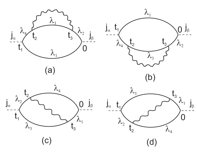
FIG. 2.: The four first order diagrams. The time ordering is as follows: $t_{1}>t_{2}>t_{3}>0$.

A General Results

The perturbation theory can be constructed by means of a regular expansion of the kernel of the evolution operator $J$ (A38) in powers of $iS_{R}+S_{I}$. In the first order one obtains four diagrams presented in Fig. 2. The contribution of the self-energy diagrams (Fig. 2a,b) was analyzed in details in Appendix A. It was demonstrated that this contribution to $\delta\sigma$ can be written in terms of the the evolution operator $U$ for noninteracting electrons. The corresponding expression is defined in (A32-A35). It is equivalent to the result (A5) obtained diagrammatically by AAG.

Let us express the evolution operator $U$ in the basis of the exact wave functions of noninteracting electrons:

$$U(t,\mathchoice{{\hbox{\boldmath$\displaystyle r$}}}{{\hbox{\boldmath$\textstyle r$}}}{{\hbox{\boldmath$\scriptstyle r$}}}{{\hbox{\boldmath$\scriptscriptstyle r$}}}_{1},\mathchoice{{\hbox{\boldmath$\displaystyle r$}}}{{\hbox{\boldmath$\textstyle r$}}}{{\hbox{\boldmath$\scriptstyle r$}}}{{\hbox{\boldmath$\scriptscriptstyle r$}}}_{2})=\langle\mathchoice{{\hbox{\boldmath$\displaystyle r$}}}{{\hbox{\boldmath$\textstyle r$}}}{{\hbox{\boldmath$\scriptstyle r$}}}{{\hbox{\boldmath$\scriptscriptstyle r$}}}_{1}|\exp(-i\hat{H}_{0}t)|\mathchoice{{\hbox{\boldmath$\displaystyle r$}}}{{\hbox{\boldmath$\textstyle r$}}}{{\hbox{\boldmath$\scriptstyle r$}}}{{\hbox{\boldmath$\scriptscriptstyle r$}}}_{2}\rangle=\sum\limits_{\lambda}e^{-i\xi_{\lambda}t}\psi_{\lambda}(\mathchoice{{\hbox{\boldmath$\displaystyle r$}}}{{\hbox{\boldmath$\textstyle r$}}}{{\hbox{\boldmath$\scriptstyle r$}}}{{\hbox{\boldmath$\scriptscriptstyle r$}}}_{1})\psi^{*}_{\lambda}(\mathchoice{{\hbox{\boldmath$\displaystyle r$}}}{{\hbox{\boldmath$\textstyle r$}}}{{\hbox{\boldmath$\scriptstyle r$}}}{{\hbox{\boldmath$\scriptscriptstyle r$}}}_{2}).$$ (63)

Obviously the representation (63) holds both with and without the external magnetic field with the only difference that in the latter case the energy levels are doubly degenerate, while in the former case this degeneracy is lifted by the magnetic field.

The density matrix $\rho$ which enters the expression (A32) can also be expanded in the basis of the eigenfunctions $\psi_{\lambda}$. We find

$$(1-2\rho)(\mathchoice{{\hbox{\boldmath$\displaystyle r$}}}{{\hbox{\boldmath$\textstyle r$}}}{{\hbox{\boldmath$\scriptstyle r$}}}{{\hbox{\boldmath$\scriptscriptstyle r$}}}_{1},\mathchoice{{\hbox{\boldmath$\displaystyle r$}}}{{\hbox{\boldmath$\textstyle r$}}}{{\hbox{\boldmath$\scriptstyle r$}}}{{\hbox{\boldmath$\scriptscriptstyle r$}}}_{2})=\sum\limits_{\lambda}\tanh\frac{\xi_{\lambda}}{2T}\psi_{\lambda}(\mathchoice{{\hbox{\boldmath$\displaystyle r$}}}{{\hbox{\boldmath$\textstyle r$}}}{{\hbox{\boldmath$\scriptstyle r$}}}{{\hbox{\boldmath$\scriptscriptstyle r$}}}_{1})\psi^{*}_{\lambda}(\mathchoice{{\hbox{\boldmath$\displaystyle r$}}}{{\hbox{\boldmath$\textstyle r$}}}{{\hbox{\boldmath$\scriptstyle r$}}}{{\hbox{\boldmath$\scriptscriptstyle r$}}}_{2}),$$ (64)

$$\frac{\partial\rho}{\partial\mu}(\mathchoice{{\hbox{\boldmath$\displaystyle r$}}}{{\hbox{\boldmath$\textstyle r$}}}{{\hbox{\boldmath$\scriptstyle r$}}}{{\hbox{\boldmath$\scriptscriptstyle r$}}}_{1},\mathchoice{{\hbox{\boldmath$\displaystyle r$}}}{{\hbox{\boldmath$\textstyle r$}}}{{\hbox{\boldmath$\scriptstyle r$}}}{{\hbox{\boldmath$\scriptscriptstyle r$}}}_{2})=\sum\limits_{\lambda}\frac{1}{2}\left(\frac{d}{d\xi_{\lambda}}\tanh\frac{\xi_{\lambda}}{2T}\right)\psi_{\lambda}(\mathchoice{{\hbox{\boldmath$\displaystyle r$}}}{{\hbox{\boldmath$\textstyle r$}}}{{\hbox{\boldmath$\scriptstyle r$}}}{{\hbox{\boldmath$\scriptscriptstyle r$}}}_{1})\psi^{*}_{\lambda}(\mathchoice{{\hbox{\boldmath$\displaystyle r$}}}{{\hbox{\boldmath$\textstyle r$}}}{{\hbox{\boldmath$\scriptstyle r$}}}{{\hbox{\boldmath$\scriptscriptstyle r$}}}_{2}).$$ (65)

Now let us substitute (63-65) into the expression (A32). Performing the two time integrals after a straightforward algebra (see Appendix B for details) we obtain the correction to the conductivity due to the self-energy diagrams of Fig. 2a,b

$$\delta\sigma^{\rm se}_{\alpha\beta} = \delta\sigma_{\alpha\beta}^{C}-\frac{e^{2}}{2\cal{V}\sigma}\int\limits_{0}^{+\infty}dt_{1}\sum\limits_{\lambda_{1}..\lambda_{4}}\left(\frac{d}{d\xi_{\lambda_{1}}}\tanh\frac{\xi_{\lambda_{1}}}{2T}\right)\left(j^{\lambda_{4}\lambda_{1}}_{\alpha}j^{\lambda_{1}\lambda_{2}}_{\beta}+j^{\lambda_{4}\lambda_{1}}_{\beta}j^{\lambda_{1}\lambda_{2}}_{\alpha}\right)M^{\lambda_{2}\lambda_{3};\lambda_{3}\lambda_{4}}\times$$ (67)

$$\int\frac{d\omega}{2\pi}\;\;\omega\left[\coth\frac{\omega}{2T}+\tanh\frac{\xi_{\lambda_{3}}}{2T}\right]F(t_{1},\omega,\xi_{\lambda_{1}}..\xi_{\lambda_{4}}),$$

where we defined the matrix elements

$$j^{\lambda_{1}\lambda_{2}}_{\alpha}=\int d\mathchoice{{\hbox{\boldmath$\displaystyle r$}}}{{\hbox{\boldmath$\textstyle r$}}}{{\hbox{\boldmath$\scriptstyle r$}}}{{\hbox{\boldmath$\scriptscriptstyle r$}}}\psi^{*}_{\lambda_{1}}(\mathchoice{{\hbox{\boldmath$\displaystyle r$}}}{{\hbox{\boldmath$\textstyle r$}}}{{\hbox{\boldmath$\scriptstyle r$}}}{{\hbox{\boldmath$\scriptscriptstyle r$}}})\hat{j}_{\alpha}\psi_{\lambda_{2}}(\mathchoice{{\hbox{\boldmath$\displaystyle r$}}}{{\hbox{\boldmath$\textstyle r$}}}{{\hbox{\boldmath$\scriptstyle r$}}}{{\hbox{\boldmath$\scriptscriptstyle r$}}}),\;\;\;\;M^{\lambda_{2}\lambda_{3};\lambda_{3}\lambda_{4}}=\int\frac{d^{3}k}{(2\pi)^{3}}\;\;\frac{1}{k^{2}}\langle\lambda_{2}|e^{i\mathchoice{{\hbox{\boldmath$\displaystyle kr$}}}{{\hbox{\boldmath$\textstyle kr$}}}{{\hbox{\boldmath$\scriptstyle kr$}}}{{\hbox{\boldmath$\scriptscriptstyle kr$}}}}|\lambda_{3}\rangle\langle\lambda_{3}|e^{-i\mathchoice{{\hbox{\boldmath$\displaystyle kr$}}}{{\hbox{\boldmath$\textstyle kr$}}}{{\hbox{\boldmath$\scriptstyle kr$}}}{{\hbox{\boldmath$\scriptscriptstyle kr$}}}}|\lambda_{4}\rangle$$ (68)

and the function

$$F(t_{1},\omega,\xi_{\lambda_{1}}..\xi_{\lambda_{4}}) = \int\limits_{0}^{t_{1}}dt_{2}\int\limits_{0}^{t_{2}}dt_{3}\cos(-\xi_{\lambda_{1}}t_{1}+\xi_{\lambda_{2}}t_{3}+(\xi_{\lambda_{3}}+\omega)(t_{2}-t_{3})+\xi_{\lambda_{4}}(t_{1}-t_{2}))$$ (69)

$$= \cos\xi_{21}t_{1}\frac{\xi_{42}[\cos((\xi_{32}+\omega)t_{1})-1]+(\xi_{32}+\omega)[1-\cos\xi_{42}t_{1}]}{\xi_{42}(\xi_{42}-\xi_{32}-\omega)(\xi_{32}+\omega)}$$ (71)

$$-\sin\xi_{21}t_{1}\frac{\xi_{42}\sin((\xi_{32}+\omega)t_{1})-(\xi_{32}+\omega)\sin\xi_{42}t_{1}}{\xi_{42}(\xi_{42}-\xi_{32}-\omega)(\xi_{32}+\omega)}.$$

Here we introduced the notation $\xi_{ij}\equiv\xi_{\lambda_{i}}-\xi_{\lambda_{j}}$.

The term $\delta\sigma_{\alpha\beta}^{C}$ in (67) describes the correction due to the non-screened Coulomb interaction. It is defined by the following expression:

$$\delta\sigma_{\alpha\beta}^{C} = -\frac{e^{2}}{4{\cal{V}}}\int\limits_{0}^{+\infty}dt_{1}\int\limits_{0}^{t_{1}}dt_{2}\sum\limits_{\lambda_{1},\lambda_{2},\lambda_{4}}\left(\frac{d}{d\xi_{\lambda_{1}}}\tanh\frac{\xi_{\lambda_{1}}}{2T}\right)\left(j_{\alpha}^{\lambda_{4}\lambda_{1}}j_{\beta}^{\lambda_{1}\lambda_{2}}+j_{\beta}^{\lambda_{4}\lambda_{1}}j_{\alpha}^{\lambda_{1}\lambda_{2}}\right)\times$$ (73)

$$\times\left\langle\lambda_{2}\right|\frac{[1-2\rho](\mathchoice{{\hbox{\boldmath$\displaystyle r$}}}{{\hbox{\boldmath$\textstyle r$}}}{{\hbox{\boldmath$\scriptstyle r$}}}{{\hbox{\boldmath$\scriptscriptstyle r$}}}_{1},\mathchoice{{\hbox{\boldmath$\displaystyle r$}}}{{\hbox{\boldmath$\textstyle r$}}}{{\hbox{\boldmath$\scriptstyle r$}}}{{\hbox{\boldmath$\scriptscriptstyle r$}}}_{2})}{|\mathchoice{{\hbox{\boldmath$\displaystyle r$}}}{{\hbox{\boldmath$\textstyle r$}}}{{\hbox{\boldmath$\scriptstyle r$}}}{{\hbox{\boldmath$\scriptscriptstyle r$}}}_{1}-\mathchoice{{\hbox{\boldmath$\displaystyle r$}}}{{\hbox{\boldmath$\textstyle r$}}}{{\hbox{\boldmath$\scriptstyle r$}}}{{\hbox{\boldmath$\scriptscriptstyle r$}}}_{2}|}\left|\lambda_{4}\right\rangle\sin[-\xi_{\lambda_{1}}t_{1}+\xi_{\lambda_{2}}t_{2}+\xi_{\lambda_{4}}(t_{1}-t_{2})].$$

The contribution to $\delta\sigma$ from the vertex diagrams of Fig. 2c,d can be found analogously (see Appendix B). We get

$$\delta\sigma_{\alpha\beta}^{\rm vert} = -\frac{e^{2}}{2{\cal V}\sigma}\int\limits_{0}^{\infty}dt_{1}\sum\limits_{\lambda_{1}..\lambda_{4}}\left(\frac{d}{d\xi_{\lambda_{1}}}\tanh\frac{\xi_{\lambda_{1}}}{2T}\right)\left(j_{\alpha}^{\lambda_{2}\lambda_{3}}j_{\beta}^{\lambda_{1}\lambda_{4}}+j_{\beta}^{\lambda_{2}\lambda_{3}}j_{\alpha}^{\lambda_{1}\lambda_{4}}\right)M^{\lambda_{3}\lambda_{1};\lambda_{4}\lambda_{2}}$$ (75)

$$\times\int\frac{d\omega}{2\pi}\;\;\omega\left[-\coth\frac{\omega}{2T}+\tanh\frac{\xi_{\lambda_{3}}}{2T}\right]G(t_{1},\omega,\xi_{\lambda_{1}}..\xi_{\lambda_{4}}).$$

Here we have introduced the following function:

$$G(t_{1},\omega,\xi_{\lambda_{1}}..\xi_{\lambda_{4}}) = \int\limits_{0}^{t_{1}}dt_{2}\int\limits_{0}^{t_{2}}dt_{3}\cos(-\xi_{\lambda_{3}}(t_{1}-t_{3})-\xi_{\lambda_{1}}t_{3}+\xi_{\lambda_{4}}t_{2}+\xi_{\lambda_{2}}(t_{1}-t_{2})+\omega(t_{2}-t_{3}))$$ (76)

$$= \cos\xi_{21}t_{1}\frac{(\xi_{42}+\xi_{31})\cos[(\xi_{31}-\xi_{42}-\omega)t_{1}]-(\xi_{42}+\omega)\cos\xi_{42}t_{1}-(\xi_{31}-\omega)\cos\xi_{31}t_{1}}{(\xi_{42}+\xi_{31})(\xi_{31}-\omega)(\xi_{42}+\omega)}$$ (78)

$$+\sin\xi_{21}t_{1}\frac{(\xi_{42}+\xi_{31})\sin[(\xi_{31}-\xi_{42}-\omega)t_{1}]+(\xi_{42}+\omega)\sin\xi_{42}t_{1}-(\xi_{31}-\omega)\sin\xi_{31}t_{1}}{(\xi_{42}+\xi_{31})(\xi_{31}-\omega)(\xi_{42}+\omega)}.$$

Despite an obvious similarity in the structure of the self-energy (eq. (67)) and the vertex (eq. (75)) corrections to the conductivity these two expressions differ in several aspects: the terms containing $\coth(\omega/2T)$ in (67) and (75) have the opposite signs, the functions $F$ (69) and $G$ (76) of the energy arguments $\xi_{\lambda}$ are different and the matrix elements entering (67) and (75) depend on different indices.

It is important to emphasize that the eqs. (67-76) determine the total correction to the conductivity tensor $\sigma_{\alpha\beta}=\sigma^{\rm se}_{\alpha\beta}+\sigma^{\rm vert}_{\alpha\beta}$ which is identical to the initial results (A5) and (A32). In deriving (67-76) from (A32) no quasiclassical approximation, no averaging over disorder and/or no other approximation of any kind has been made: the above equations are exact quantum mechanical results in the first order in the interaction. Therefore these equations can be conveniently used to test the statement about the full cancellation of the first order diagrams at $T\to 0$ which is quite frequently made in the literature (see e.g. [26] as well as recent works [17, 18] and further references therein).

B Breakdown of the Fermi Golden Rule Approximation

Although here we are mainly interested in the contribution of the diagrams of Fig. 2 to the current-current correlation function, the structure of the result is by no means specific to this function only. The very same structure – perhaps apart from the matrix elements of the current operator – is reproduced if one calculates e.g. the inelastic scattering time [26, 27, 18] and similar quantities. This is quite natural because the results for different quantities follow from the expansion of the same evolution operator $J$ (A38) in the interaction. Hence, the analysis to be presented below is general and can be applied to various physical quantities evaluated by means of the diagrams of Fig. 2.

Let us consider the self-energy diagrams of Fig. 2a,b. Just for the sake of clarity let us repeat the statement we are going to test: according to Fukuyama and Abrahams [26] and to some other authors the contribution of these diagrams vanishes in the limit $T\to 0$ because the result contains the combination

$$\left(\frac{d}{d\epsilon}\tanh\frac{\epsilon}{2T}\right)\left[\coth\frac{\omega}{2T}+\tanh\frac{\epsilon-\omega}{2T}\right]$$ (79)

under the integrals over $\epsilon$ and $\omega$. This combination restricts both integrals to the regions $|\epsilon|\lesssim T$ and $|\omega|\lesssim T$ and makes the result to vanish completely at $T=0$.

Already the first inspection of the expression (67,69) allows to observe that it is the combination

$$\left(\frac{d}{d\xi_{\lambda_{1}}}\tanh\frac{\xi_{\lambda_{1}}}{2T}\right)\left[\coth\frac{\omega}{2T}+\tanh\frac{\xi_{\lambda_{3}}}{2T}\right].$$ (80)

and not (79) which enters the exact quantum mechanical result. This combination is not zero even at $T=0$ because $\xi_{\lambda_{3}}\not=\xi_{\lambda_{1}}-\omega$, high frequencies $|\omega|>T$ do contribute to the integral and, moreover, this integral may – depending on the spectrum of the fluctuation propagator – even diverge for large $\omega$ unless one introduces an effective high frequency cutoff. We would like to emphasize that these conclusions are general and do not depend on any particular form of the matrix elements (68). Thus the statement of the above papers that the contribution of the diagrams of Fig. 2a,b vanishes in equilibrium at $T=0$ is proven to be incorrect. Below we will demonstrate that this poorly justified statement is a result of several rough approximations, the main of which is the golden rule approximation. This approximation may sometimes yield correct leading order results in the high temperature limit, but it breaks down at sufficiently low $T$.

In order to illustrate this point let us first make a simplifying assumption. Namely, let us for a moment restrict our attention only to the contribution of the terms with $\xi_{\lambda_{1}}=\xi_{\lambda_{2}}=\xi_{\lambda_{4}}$. Below we will see that this assumption is not sufficient to properly evaluate the first order perturbation correction to the conductivity: in order to do that it is important to allow for a (possibly small) difference between $\xi_{\lambda_{1}}$ and $\xi_{\lambda_{2}}$. But such an approximation is sufficient for calculation of some other physical quantities, like the inelastic scattering time, and we will adopt it for a moment just in order to demonstrate the failure of the golden-rule-type perturbation theory in the interaction.

The contribution of the terms with $\xi_{\lambda_{1}}=\xi_{\lambda_{2}}=\xi_{\lambda_{4}}$ to the conductivity $\delta\sigma^{\rm se}$ reads

$$\delta\tilde{\sigma}_{\alpha\beta}^{\rm se} = -\frac{e^{2}}{2\cal{V}\sigma}\int\limits_{0}^{+\infty}dt_{1}\sum\limits_{\lambda_{1}..\lambda_{4}}^{\xi_{\lambda_{1}}=\xi_{\lambda_{2}}=\xi_{\lambda_{4}}}\left(\frac{d}{d\xi_{\lambda_{1}}}\tanh\frac{\xi_{\lambda_{1}}}{2T}\right)\left(j^{\lambda_{4}\lambda_{1}}_{\alpha}j^{\lambda_{1}\lambda_{2}}_{\beta}+j^{\lambda_{4}\lambda_{1}}_{\beta}j^{\lambda_{1}\lambda_{2}}_{\alpha}\right)M^{\lambda_{2}\lambda_{3};\lambda_{3}\lambda_{4}}\times$$ (82)

$$\int\frac{d\omega}{2\pi}\;\;\omega\left[\coth\frac{\omega}{2T}+\tanh\frac{\xi_{\lambda_{3}}}{2T}\right]\frac{1-\cos((\xi_{31}+\omega)t_{1})}{(\xi_{31}+\omega)^{2}}.$$

Let us first evaluate this expression within the Fermi golden rule approximation:

$$\frac{1-\cos((\xi_{31}+\omega)t_{1})}{(\xi_{31}+\omega)^{2}}\longrightarrow\pi t_{1}\delta(\xi_{31}+\omega).$$ (83)

Substituting (83) into (82) we obtain

$$\delta\tilde{\sigma}_{\alpha\beta}^{\rm se,\;GR} = -\frac{e^{2}}{4\cal{V}\sigma}\int\limits_{0}^{+\infty}dt_{1}\;\;t_{1}\sum\limits_{\lambda_{1}..\lambda_{4}}^{\xi_{\lambda_{1}}=\xi_{\lambda_{2}}=\xi_{\lambda_{4}}}\left(\frac{d}{d\xi_{\lambda_{1}}}\tanh\frac{\xi_{\lambda_{1}}}{2T}\right)\left(j^{\lambda_{4}\lambda_{1}}_{\alpha}j^{\lambda_{1}\lambda_{2}}_{\beta}+j^{\lambda_{4}\lambda_{1}}_{\beta}j^{\lambda_{1}\lambda_{2}}_{\alpha}\right)M^{\lambda_{2}\lambda_{3};\lambda_{3}\lambda_{4}}\times$$ (85)

$$\xi_{31}\left[\coth\frac{\xi_{31}}{2T}-\tanh\frac{\xi_{\lambda_{3}}}{2T}\right]\propto T\int\limits_{0}^{+\infty}dt_{1}\;\;t_{1}.$$

This expression implies that within the Fermi golden rule approximation the self-energy diagrams of Fig. 2a,b yield a linear in time decay of the initial quantum state with the corresponding relaxation rate proportional to $T$. Obviously, such relaxation rate vanishes at $T=0$ in agreement with Ref. [26] and others.

Now let us carry out an exact frequency integration in (82) without making the golden rule approximation (83). It is fairly obvious that the integral over $\omega$ is not restricted to $|\omega|\lesssim T$ and even diverges at high frequencies. As before, in order to cure this divergence we introduce the high frequency cutoff $\omega_{c}\approx 1/\tau_{e}$. For simplicity we also assume that the energy difference $\xi_{31}$ is smaller than $1/\tau_{e}$. Then in the limit $T\to 0$ we find

$$\int\frac{d\omega}{2\pi}\omega\left[\coth\frac{\omega}{2T}+\tanh\frac{\xi_{\lambda_{3}}}{2T}\right]_{T\to 0}\frac{1-\cos((\xi_{31}+\omega)t_{1})}{(\xi_{31}+\omega)^{2}}$$

$$=\frac{|\xi_{31}|t_{1}}{2}-\frac{\xi_{31}t_{1}}{2}{\rm sign}\xi_{\lambda_{3}}+2\int\limits_{|\xi_{31}|}^{1/\tau_{e}}\frac{d\omega}{2\pi}\left(\frac{1}{\omega}-\frac{|\xi_{31}|}{\omega^{2}}\right)\left(1-\cos\omega t_{1}\right).$$ (86)

The first and the third terms in the second line of this expression come from $\coth(\omega/2T)$ while the second term originates from $\tanh(\xi_{\lambda_{3}}/2T)$. We observe that the first two terms are the same as in the golden rule approximation (85). These terms enter with the opposite signs and exactly cancel each other at $T=0$ because in this limit $(d/d\xi_{\lambda_{1}})\tanh(\xi_{\lambda_{1}}/2T)$ reduces to a $\delta$-function and therefore $\xi_{\lambda_{3}}\equiv\xi_{31}$. The last term does not vanish even at zero temperature, this term is not small and obviously contains the contribution of all frequencies up to $1/\tau_{e}$. The integral over $\omega$ contained in this term can be easily evaluated. We will do it a bit later when we fix the dependence of the matrix elements $M^{\lambda_{2},\lambda_{3};\lambda_{3},\lambda_{4}}$ on energies. Now it is only important for us to demonstrate that the last term in (86) is completely missing within the golden rule approach employed in Refs. [26, 17, 18] and others. It is obvious, therefore, that this approach fails to correctly describe the system behavior at sufficiently low temperatures.

Note, that AAG [13] also did not observe an exact cancellation of diagrams of the first order perturbation theory in the interaction. However, they argued that the remaining terms provide the so-called interaction correction to the conductance which can be viewed as an effective (temperature dependent) renormalization of the bare parameters and has nothing to do with dephasing. Already from the form of the third term in the right hand side of (86) one can conclude that in general this is not true. Indeed, if one adopts that for $\xi_{\lambda_{1}}=\xi_{\lambda_{2}}=\xi_{\lambda_{4}}$ the dependence of the matrix elements $M^{\lambda_{2},\lambda_{3};\lambda_{3},\lambda_{4}}$ on the energy difference $\xi_{31}$ has the form

$$M^{\lambda_{2},\lambda_{3};\lambda_{3},\lambda_{4}}\propto|\xi_{31}|^{d/2-2}$$ (87)

(cf. eq. (2.33) of Ref. [13]), and integrates the product of $M^{\lambda_{2},\lambda_{3};\lambda_{3},\lambda_{4}}$ and the last term in (86) over the energy $\xi_{31}$ one immediately observes that after the cancellation of the unphysical divergence (which is also contained in the vertex diagrams of Fig. 2c,d and enters with the opposite sign, see also Section 3a) one obtains the contribution $\propto\sqrt{t}\ln(t/\tau_{e})$ in 1d and $\ln(t/\tau_{e})$ in 2d. This contribution is just a part of the function $\delta f_{d}(T,t)$ (36) at $T\to 0$. It grows with time, contributes to dephasing and obviously cannot be reduced to the renormalization of the initial parameters which would be provided by a time-independent term.

In order to understand why AAG arrived at such a conclusion it is appropriate to highlight the approximation employed in Ref. [13]. As a first step they split the total contribution to $\delta\sigma$ into two parts, eqs. (5.12c) and (5.12d), effectively rewriting the combination (80) in the following equivalent form:

$$\left(\frac{d}{d\xi_{\lambda_{1}}}\tanh\frac{\xi_{\lambda_{1}}}{2T}\right)\left[\left(\coth\frac{\omega}{2T}+\tanh\frac{\xi_{\lambda_{1}}-\omega}{2T}\right)+\left(\tanh\frac{\xi_{\lambda_{3}}}{2T}-\tanh\frac{\xi_{\lambda_{1}}-\omega}{2T}\right)\right].$$ (88)

The first two terms in the square brackets of (88) were interpreted by AAG as a “dephasing” contribution (eq. (5.12c) of [13]) while the last two terms are meant to be the “interaction” correction (eq. (5.12d) of [13]). Obviously, the contribution of the first two terms vanishes at $T\to 0$. In order to understand the behavior of the remaining terms we make use of (82), (87) and observe that the contribution of the last two terms in (88) is proportional to the following integral

$$\int d\omega\int d\xi_{\lambda_{1}}\int d\xi_{\lambda_{3}}\left(\frac{d}{d\xi_{\lambda_{1}}}\tanh\frac{\xi_{\lambda_{1}}}{2T}\right)\omega|\xi_{31}|^{d/2-2}\left[\tanh\frac{\xi_{\lambda_{3}}}{2T}-\tanh\frac{\xi_{\lambda_{1}}-\omega}{2T}\right]\frac{1-\cos((\xi_{31}+\omega)t)}{(\xi_{31}+\omega)^{2}}.$$ (89)

The approximation employed by AAG while evaluating such a combination is equivalent to ignoring the oscillating $\cos$-term in (89). After dropping this term and making the integral dimensionless one can easily observe that the remaining integral has the form

$$A_{1}/\sqrt{T}$$ (90)

in 1d and $A_{2}\ln T$ in 2d, where $A_{1,2}$ are temperature- and time-independent constants. AAG interpreted these contributions as an effective renormalization due to interaction. Note, however, that it is correct to drop the $\cos$-term only at sufficiently long times $Tt\gg 1$, while at smaller $Tt\lesssim 1$ this term is important. Evaluation of the integral (89) in the latter limit yields

$$B_{1}\sqrt{t}\ln(t/\tau_{e})$$ (91)

in 1d and $B_{2}\ln(t/\tau_{e})$ in 2d, where $B_{1,2}$ are again temperature- and time-independent constants. It is fairly obvious that the term (91) already cannot be interpreted as a renormalization effect from an effective static potential. This term explicitly depends on time and actually contributes to dephasing!

Now we are aware of the behavior of the integral (89) at all times: at $t=0$ this integral is obviously zero, it grows with time as (91) for $Tt\lesssim 1$, reaches the value (90) and saturates in the long time limit $Tt\gg 1$. Clearly, in the interesting limit $T\to 0$ the behavior (90) can never be realized, the term (89) grows at all times and contributes to dephasing. In this limit we are back to the result (86). The perturbation theory strongly diverges in this case. It also diverges at finite temperatures, thus the corresponding expressions can only make sense if one introduces a cutoff at times much smaller than the dephasing time $\tau_{\varphi}$, because at times $t\sim\tau_{\varphi}$ all orders of the perturbation theory should be taken into account. In Ref. [13] this cutoff time was chosen to be the magnetic-field-induced decoherence time $\tau_{H}\ll\tau_{\varphi}$. Thus the approximation leading to the time-independent term (90) is valid only for $T\tau_{H}\gg 1$, in which case the contribution (91) is anyway much smaller than that from the first two terms in (88) and, hence, can be safely ignored in the above limit. On the other hand, in the most interesting limit $T\tau_{H}\lesssim 1$ (which is compatible with $T\tau_{\varphi}\gg 1$) the contribution (89) dominates, its behavior is given by eq. (91) rather than by eq. (90) and, consequently, nonzero low temperature dephasing is observed already in the first order perturbation theory in the interaction. We will come back to this discussion in Sec. 4.D and in Appendix C.

Let us emphasize again that no approximation was done during our derivation presented in Sec. 4A. Our main goal here was to demonstrate that the absence of the cancellation of diagrams in the first order perturbation theory has nothing to do with the quasiclassical approximation and/or disorder average as it is sometimes speculated in the literature.

C Perturbative weak localization correction

Now let us perform a systematic evaluation of the exact expressions (67)-(76) obtained within the first order perturbation theory in the interaction. Our calculation consists of several steps. First we notice that the expressions (67)-(76) contain the full information about contributions from all energy states. Since here we are interested only in the weak localization correction to the conductance we should restrict our attention to the time reversed energy states and evaluate the matrix elements for such states. The matrix elements for the current operator can be extracted from the expression for the weak localization correction without interaction $\delta\sigma_{\alpha\beta}^{{\rm ni}}$. Starting from the standard expression for this correction (see e.g. Ref. [13]) and rewriting it in terms of the matrix elements for the current (68) we obtain

$$\delta\sigma_{\alpha\beta}^{{\rm ni}} = \frac{1}{8}\int\frac{d\mathchoice{{\hbox{\boldmath$\displaystyle r$}}}{{\hbox{\boldmath$\textstyle r$}}}{{\hbox{\boldmath$\scriptstyle r$}}}{{\hbox{\boldmath$\scriptscriptstyle r$}}}_{1}}{\mathchoice{{\hbox{\boldmath$\displaystyle r$}}}{{\hbox{\boldmath$\textstyle r$}}}{{\hbox{\boldmath$\scriptstyle r$}}}{{\hbox{\boldmath$\scriptscriptstyle r$}}}_{2}}\int\frac{d\epsilon}{2\pi}\left(\frac{d}{d\epsilon}\tanh\frac{\epsilon}{2T}\right)\left\{[G_{12}^{R}(\epsilon)-G_{12}^{A}(\epsilon)]\hat{j}_{\alpha}[G_{21}^{A}(\epsilon)-G_{21}^{R}(\epsilon)]\hat{j}_{\beta}+\alpha\leftrightarrow\beta\right\}$$ (92)

$$= \frac{1}{4{\cal V}}\int\limits_{0}^{+\infty}dt_{1}\sum\limits_{\lambda_{1}\lambda_{2}}\left(\frac{d}{d\xi_{\lambda_{1}}}\tanh\frac{\xi_{\lambda_{1}}}{2T}\right)\left(j_{\alpha}^{\lambda_{1}\lambda_{2}}j_{\beta}^{\lambda_{2}\lambda_{1}}+j_{\beta}^{\lambda_{1}\lambda_{2}}j_{\alpha}^{\lambda_{2}\lambda_{1}}\right)\cos\xi_{21}t_{1}.$$ (93)

The expression for the matrix elements of the currents $jj(\xi_{21})$ is readily established by comparison (93) to the well known quasiclassical result in the absence of interaction (6). We find

$$jj(\xi_{21}) = j_{\alpha}^{\lambda_{1}\lambda_{2}}j_{\beta}^{\lambda_{2}\lambda_{1}}+j_{\beta}^{\lambda_{1}\lambda_{2}}j_{\alpha}^{\lambda_{2}\lambda_{1}}=-\frac{4e^{2}D{\cal V}}{\pi^{2}}\int\frac{d^{d}Q}{(2\pi)^{d}}\;\frac{DQ^{2}+1/\tau_{H}}{\xi_{21}^{2}+(DQ^{2}+1/\tau_{H})^{2}}$$ (94)

$$= \left\{\begin{array}[]{ll}-\frac{2e^{2}{\cal V}}{\pi^{2}}\sqrt{D\tau_{H}}{\rm Re}\left(\frac{1}{\sqrt{1+i|\xi_{21}|\tau_{H}}}\right),&{\rm 1d}\\ -\frac{e^{2}{\cal V}}{\pi^{3}}\left(\ln\frac{\tau_{H}}{\tau_{e}}-\frac{1}{2}\ln(1+(\xi_{21}\tau_{H})^{2})\right),&{\rm 2d}\end{array}\right.$$ (97)

As it was already pointed out above, these expressions are only valid for the time reversed states $\lambda_{1}$ and $\lambda_{2}$ relevant for the weak localization correction. For later purposes let us also rewrite the above result in the 1d case in the real time representation:

$$\int d\xi_{21}jj(\xi_{21})\cos\xi_{21}t_{1}=-\frac{4{\cal V}e^{2}}{2\pi}\sqrt{\frac{D}{\pi}}\frac{e^{-|t_{1}|/\tau_{H}}}{\sqrt{|t_{1}|}}.$$ (98)

The next step in our calculation is to identify the contribution to $\delta\sigma$ responsible for dephasing. As it was already demonstrated above within the nonperturbative analysis, this contribution is determined by the function $f_{d}(t)$ (24) in the exponent (6). Clearly, in the first order in the interaction this contribution is obtained by expanding the exponent in (6) up to the linear term in $f_{d}(t)$ and ignoring the effect of interaction on the pre-exponential function $A_{d}(t)$. Hence, this “dephasing” contribution should have the form

$$\delta\sigma_{\alpha\beta}^{\rm deph}=\frac{1}{4{\cal V}}\int\limits_{0}^{+\infty}dt_{1}\;\;f_{d}(t_{1})\sum\limits_{\lambda_{1}\lambda_{2}}\left(\frac{d}{d\xi_{\lambda_{1}}}\tanh\frac{\xi_{\lambda_{1}}}{2T}\right)\left(j_{\alpha}^{\lambda_{1}\lambda_{2}}j_{\beta}^{\lambda_{2}\lambda_{1}}+j_{\beta}^{\lambda_{1}\lambda_{2}}j_{\alpha}^{\lambda_{2}\lambda_{1}}\right)\cos\xi_{21}t_{1}.$$ (99)

We observe that this expression contains the function $\cos\xi_{21}t_{1}$ and does not contain $\sin\xi_{21}t_{1}$. Furthermore, from the above analysis we know that the function $f_{d}(t)$ contains only $\coth(\omega/2T)$ and does not depend on $\tanh(\xi_{\lambda_{3}}/2T)$. Therefore in the general result for the conductance correction (67)-(76) we will first take care of all terms which contain the product $\coth(\omega/2T)\cos\xi_{21}t_{1}$ leaving all the remaining terms for further consideration.

Consider the “coth$\times$cos” terms originating from the self-energy diagrams of Fig. 2a,b. For such diagrams one should put $\xi_{42}=0$, then from (67), (69) one will immediately observe that the contribution of the “coth$\times$cos” terms can indeed be represented in the form (99) where

$$f^{\rm se}_{d}(t,\lambda_{2})=\frac{2e^{2}}{\sigma}\sum\limits_{\lambda_{3}}\int\frac{d\omega}{2\pi}\;\;M^{\lambda_{2}\lambda_{3};\lambda_{3}\lambda_{2}}\omega\coth\frac{\omega}{2T}\frac{1-\cos[(\xi_{32}+\omega)t]}{(\xi_{32}+\omega)^{2}}.$$ (100)

Let us replace the summation over $\lambda_{3}$ by the integration over $\xi_{\lambda_{3}}$. Assuming that the matrix elements $M^{\lambda_{2}\lambda_{3};\lambda_{3}\lambda_{2}}$ depend only on the energy difference $\xi_{32}$, making a shift $\xi_{32}+\omega\to\omega$ and denoting $\xi_{32}\to\omega^{\prime}$ we find

$$f^{\rm se}_{d}(t)=\frac{4\pi e^{2}}{\sigma}\int\frac{d\omega d\omega^{\prime}}{(2\pi)^{2}}M(\omega^{\prime})(\omega-\omega^{\prime})\coth\frac{\omega-\omega^{\prime}}{2T}\;\;\frac{1-\cos\omega t}{\omega^{2}}.$$ (101)

This expression does not depend on $\lambda_{2}$ and exactly coincides with the first term in eq. (24) if we identify the matrix element $M(\omega^{\prime})$ as:

$$M(\omega^{\prime})=\frac{D^{1-d/2}}{\pi}\left(\int\frac{d^{d}x}{(2\pi)^{d}}\frac{1}{1+x^{4}}\right)|\omega^{\prime}|^{d/2-2}.$$ (102)

Note, that the energy dependence of the matrix elements $M\propto|\omega^{\prime}|^{d/2-2}$ (102) determined within the above procedure is in the agreement with the conjecture (87) as well as with eq. (2.33) of Ref. [13].

The contribution of the “coth$\times$cos” terms contained in the vertex diagrams of Fig. 2c,d can be evaluated analogously. Again one should consider only the part of the function $G$ (76) which contains $\cos(\xi_{21}t_{1})$. For the contribution of the time reversed states to the vertex diagrams one should identify $\xi_{42}=\xi_{31}$. Making use of this equation, from the corresponding terms in (75), (76) one finds

$$\delta\sigma^{{\rm deph,vert}}_{\alpha\beta} = -\frac{1}{4{\cal V}}\int\limits_{0}^{+\infty}dt_{1}f_{d}^{{\rm vert}}(t_{1},\lambda_{1})\sum\limits_{\lambda_{1}\lambda_{2}}\left(\frac{d}{d\xi_{\lambda_{1}}}\tanh\frac{\xi_{\lambda_{1}}}{2T}\right)\left(j_{\alpha}^{\lambda_{2}\lambda_{3}}j_{\beta}^{\lambda_{1}\lambda_{4}}+j_{\beta}^{\lambda_{2}\lambda_{3}}j_{\alpha}^{\lambda_{1}\lambda_{4}}\right)\cos\xi_{21}t_{1},$$ (103)

where

$$f_{d}^{{\rm vert}}(t,\lambda_{1}) = -\frac{2e^{2}}{\sigma}\sum_{\lambda_{3}}\int\frac{d\omega}{2\pi}M^{\lambda_{3}\lambda_{1};\lambda_{4}\lambda_{2}}\omega\coth\frac{\omega}{2T}\frac{\cos\omega t-\cos\xi_{31}t}{\xi_{31}^{2}-\omega^{2}}.$$ (104)

By comparing eq. (104) with the second term of the expression (24) we observe that they coincide provided one denotes $\xi_{31}=\xi_{42}=\omega^{\prime}$ and again assumes that the matrix elements depend only on the energy difference $M^{\lambda_{3}\lambda_{1};\lambda_{4}\lambda_{2}}=M(\omega^{\prime})$, where $M(\omega^{\prime})$ is defined in eq. (102). Furthermore, in order to identify eqs. (99) (with $f_{d}(t)\to f_{d}^{\rm vert}(t)$) and (103) we have to assume that $j_{\alpha}^{\lambda_{2}\lambda_{3}}j_{\beta}^{\lambda_{1}\lambda_{4}}+j_{\beta}^{\lambda_{2}\lambda_{3}}j_{\alpha}^{\lambda_{1}\lambda_{4}}=j_{\alpha}^{\lambda_{1}\lambda_{2}}j_{\beta}^{\lambda_{2}\lambda_{1}}+j_{\beta}^{\lambda_{1}\lambda_{2}}j_{\alpha}^{\lambda_{2}\lambda_{1}}$. This completes the analysis of the “coth$\times$cos”-contribution from the vertex diagrams of Fig. 2c,d.

Thus, we have explicitly demonstrated that the perturbative “dephasing” contribution to the conductance obtained before from the nonperturbative analysis can also be identified in the first order perturbative expansion provided one infers the matrix elements $M$ in the form (102). With this in mind one can immediately write down the expression for $\delta\sigma_{\alpha\beta}^{\rm deph}$ in the form (58). For a quasi-1d case at low $T$ we find

$$\delta\sigma^{\rm deph}=\frac{e^{2}}{\pi}\frac{e^{2}}{\sigma_{1}}\left[\frac{1}{\pi\sqrt{2}}\frac{D\tau_{H}^{3/2}}{\sqrt{\tau_{e}}}+\frac{2D\tau_{H}}{\pi^{2}}\left(\ln\frac{2\pi\tau_{H}}{\tau_{e}}-6-\gamma_{0}\right)\right],\;\;\;\pi T\tau_{H}\ll 1$$ (105)

In the opposite high temperature limit we obtain

$$\delta\sigma^{\rm deph}=\frac{e^{2}}{\pi}\frac{e^{2}}{\sigma_{1}}\left[\frac{4}{3\pi}DT\tau_{H}^{2}+\frac{1}{\pi\sqrt{2}}\frac{D\tau_{H}^{3/2}}{\sqrt{\tau_{e}}}+\frac{\zeta(1/2)}{\sqrt{2\pi}}D\sqrt{T}\tau_{H}^{3/2}+\frac{2D\tau_{H}}{\pi^{2}}\ln\left(\frac{1}{4T\tau_{e}}\right)-\frac{3\zeta(3/2)}{2\pi}\sqrt{\frac{D^{2}\tau_{H}}{2\pi T}}\right],\;\;\;\pi T\tau_{H}\gg 1$$ (106)

Now let us come to the final step of our calculation and evaluate the remaining terms in the general result (67)-(76). We notice that the contribution of all terms containing the combination $\coth(\omega/2T)\sin\xi_{21}t_{1}$ vanish after the integration over the energy $\xi_{21}$. The same is true for the terms containing $\tanh(\xi_{\lambda_{3}}/2T)$ in the contribution of the vertex diagrams (75). These observations imply that all the remaining nonvanishing terms come from the self-energy diagrams of Fig. 2a,b and contain $1-2\rho$ or $\tanh$. We will denote their total contribution as $\delta\sigma^{\tanh}$. We already know from the above analysis that this contribution comes from the expansion of the pre-exponent $A_{1}(t)$ to the first order in the interaction. Collecting all such terms from (67), (69) and (73), we obtain

$$\delta\sigma^{\tanh}=\delta\sigma_{\cos}^{\tanh}+\delta\sigma_{\sin}^{\tanh}+\delta\sigma^{C},$$ (107)

where

$$\delta\sigma^{\tanh}_{\cos} = -\frac{e^{2}}{2{\cal V}\sigma_{1}}\int\limits_{0}^{+\infty}dt_{1}\int d\xi_{\lambda_{1}}\int d\xi_{\lambda_{2}}\int d\xi_{\lambda_{3}}\int\frac{d\omega}{2\pi}\left(\frac{d}{d\xi_{\lambda_{1}}}\tanh\frac{\xi_{\lambda_{1}}}{2T}\right)jj(\xi_{21})\cos\xi_{21}t_{1}$$ (109)

$$\times M(\xi_{32})\omega\tanh\frac{\xi_{\lambda_{3}}}{2T}\frac{1-\cos[(\xi_{32}+\omega)t_{1}]}{(\xi_{32}+\omega)^{2}}.$$

$$\delta\sigma_{\sin}^{\tanh} = \frac{e^{2}}{2{\cal V}\sigma_{1}}\int\limits_{0}^{+\infty}dt_{1}\int d\xi_{\lambda_{1}}\int d\xi_{\lambda_{2}}\int d\xi{\lambda_{3}}\int\frac{d\omega}{2\pi}\left(\frac{d}{d\xi_{\lambda_{1}}}\tanh\frac{\xi_{\lambda_{1}}}{2T}\right)jj(\xi_{21})\sin\xi_{21}t_{1}$$ (111)

$$\ \times M(\xi_{32})\omega\tanh\frac{\xi_{\lambda_{3}}}{2T}\frac{(\xi_{32}+\omega)t_{1}-\sin(\xi_{32}+\omega)t_{1}}{(\xi_{32}+\omega)^{2}},$$

$$\delta\sigma^{C}=-\frac{e^{2}}{4{\cal{V}}}\int\limits_{0}^{+\infty}dt_{1}\ t_{1}\ \left(\frac{d}{d\xi_{\lambda_{1}}}\tanh\frac{\xi_{\lambda_{1}}}{2T}\right)jj(\xi_{21})\left\langle\lambda_{2}\right|\frac{[1-2\rho](\mathchoice{{\hbox{\boldmath$\displaystyle r$}}}{{\hbox{\boldmath$\textstyle r$}}}{{\hbox{\boldmath$\scriptstyle r$}}}{{\hbox{\boldmath$\scriptscriptstyle r$}}}_{1},\mathchoice{{\hbox{\boldmath$\displaystyle r$}}}{{\hbox{\boldmath$\textstyle r$}}}{{\hbox{\boldmath$\scriptstyle r$}}}{{\hbox{\boldmath$\scriptscriptstyle r$}}}_{2})}{|\mathchoice{{\hbox{\boldmath$\displaystyle r$}}}{{\hbox{\boldmath$\textstyle r$}}}{{\hbox{\boldmath$\scriptstyle r$}}}{{\hbox{\boldmath$\scriptscriptstyle r$}}}_{1}-\mathchoice{{\hbox{\boldmath$\displaystyle r$}}}{{\hbox{\boldmath$\textstyle r$}}}{{\hbox{\boldmath$\scriptstyle r$}}}{{\hbox{\boldmath$\scriptscriptstyle r$}}}_{2}|}\left|\lambda_{2}\right\rangle\sin\xi_{21}t_{1},$$ (112)

As before, the above equations were obtained from the exact ones by imposing $\xi_{42}=0$. In order to establish a somewhat closer relation to the approach developed by AAG we also note, that it is the contribution $\delta\sigma^{\tanh}$ (107) which contains the so-called Hikami boxes within the diagrammatic analysis of Ref. [13]. AAG argued that (partial) cancellation of the first order diagrams can only be observed if one takes the Hikami boxes into account. Below we will demonstrate that this is not the case. Actually we have already shown in Sec. 4B (eqs. (85), (86)) that this cancellation (of the linear in time “golden rule” terms only!) in the first order at $T=0$ occurs already before disorder averaging and thus has nothing to do with the Hikami boxes. Now we will illustrate this fact again by means of a direct calculation.

Let us first consider the term $\delta\sigma^{\tanh}_{\cos}$ (109). The integral over $\omega$ can be evaluated exactly and we get

$$\delta\sigma_{\cos}^{\tanh}=\frac{e^{2}}{4{\cal V}\sigma_{1}}\int\limits_{0}^{+\infty}dt_{1}\int d\xi_{\lambda_{1}}\int d\xi_{21}\int d\xi_{32}\left(\frac{d}{d\xi_{\lambda_{1}}}\tanh\frac{\xi_{\lambda_{1}}}{2T}\right)jj(\xi_{21})\cos\xi_{21}t_{1}M(\xi_{32})\xi_{32}t_{1}\tanh\frac{\xi_{\lambda_{1}}+\xi_{21}+\xi_{32}}{2T}.$$ (113)

Further calculation will be performed for a quasi-1d case. We also make use of the real time representation of our integrals, as it was already done before. For 1d systems we obtain from (102)

$$\xi_{32}M(\xi_{32})=\frac{\sqrt{D}}{2\sqrt{2}\pi}\frac{\xi_{32}}{|\xi_{32}|^{3/2}}=\frac{-i}{4\pi}\int dt^{\prime\prime}e^{i\xi_{32}t^{\prime\prime}}\left(\frac{d}{dt}\sqrt{\frac{4D|t^{\prime\prime}|}{\pi}}\right).$$ (114)

Also we will use the following relation

$$\int d\xi_{\lambda_{1}}\left(\frac{d}{d\xi_{\lambda_{1}}}\tanh\frac{\xi_{\lambda_{1}}}{2T}\right)\tanh\frac{\xi_{\lambda_{1}}+\xi_{21}+\xi_{32}}{2T}=2\pi\int dt^{\prime}e^{i(\xi_{21}+\xi_{32})t^{\prime}}\frac{Tt^{\prime}}{\sinh\pi Tt^{\prime}}{\cal P}\frac{-iT}{\sinh\pi Tt^{\prime}}.$$ (115)

Substituting (98), (114) and (115) into eq.(113), we find

$$\delta\sigma_{\cos}^{\tanh}=-\frac{e^{2}}{4\pi^{3}}\frac{e^{2}D}{\sigma_{1}}\int\limits_{0}^{+\infty}dt_{1}\int\limits_{-\infty}^{+\infty}dt^{\prime}\left({\cal P}\frac{\pi T}{\sinh\pi Tt^{\prime}}\right)\frac{\pi T}{\sinh\pi Tt^{\prime}}\;t_{1}\sqrt{|t^{\prime}|}\left[\frac{e^{-|t_{1}+t^{\prime}|/\tau_{H}}}{\sqrt{|t_{1}+t^{\prime}|}}+\frac{e^{-|t_{1}-t^{\prime}|/\tau_{H}}}{\sqrt{|t_{1}-t^{\prime}|}}\right].$$ (116)

After simple algebra this equation can be converted into the following integral:

$$\delta\sigma_{\cos}^{\tanh}=-\frac{e^{2}}{\pi^{3}}\frac{e^{2}D}{\sigma_{1}}\int\limits_{0}^{+\infty}dt\frac{e^{-t/\tau_{H}}}{\sqrt{t}}\left\{t\int\limits_{2\tau_{e}/\pi}^{t}dt^{\prime}\left(\frac{\pi T}{\sinh\pi Tt^{\prime}}\right)^{2}\sqrt{t^{\prime}}+\int\limits_{t}^{+\infty}dt^{\prime}\left(\frac{\pi T}{\sinh\pi Tt^{\prime}}\right)^{2}{t^{\prime}}^{3/2}\right\}$$ (117)

In the quantum limit $\pi T\tau_{H}\ll 1$ we get

$$\delta\sigma^{\tanh}_{\cos} = -\frac{e^{2}}{\pi^{3}}\frac{e^{2}D}{\sigma_{1}}\int\limits_{0}^{+\infty}dt\frac{e^{-t/\tau_{H}}}{\sqrt{t}}\left\{2\sqrt{\frac{\pi}{2\tau_{e}}}t-2\sqrt{t}+\frac{3\zeta(3/2)}{4\sqrt{2}}\frac{1}{\sqrt{T}}\right\}$$ (118)

$$= -\frac{e^{2}}{\pi}\frac{e^{2}}{\sigma_{1}}\left[\frac{1}{\pi\sqrt{2}}\frac{D\tau_{H}^{3/2}}{\sqrt{\tau_{e}}}-\frac{2D\tau_{H}}{\pi^{2}}+\frac{3\zeta(3/2)}{4\pi}\sqrt{\frac{D^{2}\tau_{H}}{2\pi T}}\right],\;\;\;\pi T\tau_{H}\ll 1.$$ (119)

To consider the opposite thermal limit $\pi T\tau_{H}\gg 1$ it is convenient to rewrite this equation in the following form:

$$\delta\sigma^{\tanh}_{\cos} = -\frac{e^{2}}{\pi^{3}}\frac{e^{2}D}{\sigma_{1}}\int\limits_{0}^{+\infty}dt\frac{e^{-t/\tau_{H}}}{\sqrt{t}}\left\{2t\sqrt{\frac{\pi}{2\tau_{e}}}-2\sqrt{t}\frac{\pi Tt}{\sinh\pi Tt}-4t\sqrt{\pi T}\int\limits_{0}^{\pi Tt}dx\frac{\sqrt{x}}{\sinh^{2}x}(x\coth x-1)\right.$$ (121)

$$\left.+\frac{1}{\sqrt{\pi T}}\int\limits_{\pi Tt}^{+\infty}dx\frac{x^{3/2}}{\sinh^{2}x}\right\}.$$

This equation yields

$$\delta\sigma^{\tanh}_{\cos} = -\frac{e^{2}}{\pi^{3}}\frac{e^{2}D}{\sigma_{1}}\int\limits_{0}^{+\infty}dt\frac{e^{-t/\tau_{H}}}{\sqrt{t}}\left\{2t\sqrt{\frac{\pi}{2\tau_{e}}}+\frac{\pi\zeta(1/2)}{\sqrt{2}}t\sqrt{T}\right\}$$ (122)

$$= -\frac{e^{2}}{\pi}\frac{e^{2}}{\sigma_{1}}\left[\frac{1}{\pi\sqrt{2}}\frac{D\tau_{H}^{3/2}}{\sqrt{\tau_{e}}}+\frac{\zeta(1/2)}{2\sqrt{2\pi}}D\sqrt{T}\tau_{H}^{3/2}\right],\;\;\;\pi T\tau_{H}\gg 1.$$ (123)

Here we have used the following integrals:

$$\int\limits_{0}^{+\infty}dx\frac{\sqrt{x}}{\sinh^{2}x}(x\coth x-1)=-\sqrt{\frac{\pi}{2}}\frac{\zeta(1/2)}{4},\;\;\;\;\int\limits_{0}^{+\infty}dx\frac{x^{3/2}}{\sinh^{2}x}=\sqrt{\frac{\pi}{2}}\frac{3\zeta(3/2)}{4}.$$ (124)

Now we turn to the correction (111). To begin with, we should handle a divergence which appears in the integral over $\omega$ for the term linear in $t_{1}$. It is easy to demonstrate, however, that this divergence is fictitious. It disappears completely if a more accurate expression for the matrix elements is used. This expression reads:

$$\frac{M(\xi_{32})\omega}{\sigma_{1}}=\int\frac{dk}{2\pi}\ \frac{1}{k^{2}}\left\langle\lambda_{2}\right|e^{i\mathchoice{{\hbox{\boldmath$\displaystyle kr$}}}{{\hbox{\boldmath$\textstyle kr$}}}{{\hbox{\boldmath$\scriptstyle kr$}}}{{\hbox{\boldmath$\scriptscriptstyle kr$}}}}\left|\lambda_{3}\right\rangle\left\langle\lambda_{3}\right|e^{-i\mathchoice{{\hbox{\boldmath$\displaystyle kr$}}}{{\hbox{\boldmath$\textstyle kr$}}}{{\hbox{\boldmath$\scriptstyle kr$}}}{{\hbox{\boldmath$\scriptscriptstyle kr$}}}}\left|\lambda_{2}\right\rangle\text{Im}\left(\frac{-4\pi}{\epsilon(\omega,k)}\right).$$

Now we can use the analytical properties of the function $1/\epsilon$ and write

$${\cal P}\int\frac{d\omega}{2\pi}\ \text{Im}\left(\frac{1}{\epsilon(\omega,k)}\right)\frac{1}{\xi_{32}+\omega}=\frac{1}{2}\text{Re}\left(\frac{1}{\epsilon(\xi_{23},k)}-1\right).$$

Substitution this identity into eq. (111) we immediately observe that the term containing $-1$ is exactly canceled by the correction $\delta\sigma^{C}.$ Thus the result is finite and has the form

$$\delta\sigma^{C}+\delta\sigma_{\sin}^{\tanh}=\delta\sigma_{1}^{\tanh}+\delta\sigma_{2}^{\tanh},$$ (125)

where

$$\delta\sigma_{1}^{\tanh}=-\frac{e^{2}}{4{\cal V}\sigma_{1}}\int\limits_{0}^{+\infty}dt_{1}\int d\xi_{\lambda_{1}}\int d\xi_{\lambda_{2}}\int d\xi_{\lambda_{3}}\left(\frac{d}{d\xi_{\lambda_{1}}}\tanh\frac{\xi_{\lambda_{1}}}{2T}\right)jj(\xi_{21})\sin\xi_{21}t_{1}M(\xi_{32})\tanh\frac{\xi_{\lambda_{3}}}{2T}\ .$$ (126)

and

$$\delta\sigma_{2}^{\tanh} = -\frac{e^{2}D}{4{\cal V}\sigma_{1}}\int\limits_{0}^{+\infty}dt_{1}\ t_{1}\int d\xi_{\lambda_{1}}\int d\xi_{\lambda_{2}}\int d\xi_{\lambda_{3}}\left(\frac{d}{d\xi_{\lambda_{1}}}\tanh\frac{\xi_{\lambda_{1}}}{2T}\right)jj(\xi_{21})\sin\xi_{21}t_{1}\times$$ (128)

$$\left\langle\lambda_{2}\right|_{\mathchoice{{\hbox{\boldmath$\displaystyle r$}}}{{\hbox{\boldmath$\textstyle r$}}}{{\hbox{\boldmath$\scriptstyle r$}}}{{\hbox{\boldmath$\scriptscriptstyle r$}}}_{1}}\left\langle\lambda_{3}\right|_{\mathchoice{{\hbox{\boldmath$\displaystyle r$}}}{{\hbox{\boldmath$\textstyle r$}}}{{\hbox{\boldmath$\scriptstyle r$}}}{{\hbox{\boldmath$\scriptscriptstyle r$}}}_{2}}\delta(\mathchoice{{\hbox{\boldmath$\displaystyle r$}}}{{\hbox{\boldmath$\textstyle r$}}}{{\hbox{\boldmath$\scriptstyle r$}}}{{\hbox{\boldmath$\scriptscriptstyle r$}}}_{1}-\mathchoice{{\hbox{\boldmath$\displaystyle r$}}}{{\hbox{\boldmath$\textstyle r$}}}{{\hbox{\boldmath$\scriptstyle r$}}}{{\hbox{\boldmath$\scriptscriptstyle r$}}}_{2})\left|\lambda_{3}\right\rangle_{\mathchoice{{\hbox{\boldmath$\displaystyle r$}}}{{\hbox{\boldmath$\textstyle r$}}}{{\hbox{\boldmath$\scriptstyle r$}}}{{\hbox{\boldmath$\scriptscriptstyle r$}}}_{1}}\left|\lambda_{4}\right\rangle_{\mathchoice{{\hbox{\boldmath$\displaystyle r$}}}{{\hbox{\boldmath$\textstyle r$}}}{{\hbox{\boldmath$\scriptstyle r$}}}{{\hbox{\boldmath$\scriptscriptstyle r$}}}_{2}}\tanh\frac{\xi_{\lambda_{3}}}{2T}.$$

Here we have used the formula

$${\rm Re}\left(\frac{1}{\epsilon(\xi_{23},k)}\right)=\frac{Dk^{2}}{4\pi\sigma_{1}}.$$

The contribution (126) can be transformed and evaluated analogously to the term $\delta\sigma_{\cos}^{\tanh}$. We find

$$\delta\sigma_{1}^{\tanh}=\frac{e^{2}}{2\pi^{3}}\frac{e^{2}D}{\sigma_{1}}\int\limits_{0}^{+\infty}dt_{1}\int\limits_{-\infty}^{+\infty}dt^{\prime}\left({\cal P}\frac{\pi T}{\sinh\pi Tt^{\prime}}\right)\frac{\pi T}{\sinh\pi Tt^{\prime}}\;t^{\prime}\sqrt{|t^{\prime}|}\left[\frac{e^{-|t_{1}+t^{\prime}|/\tau_{H}}}{\sqrt{|t_{1}+t^{\prime}|}}-\frac{e^{-|t_{1}-t^{\prime}|/\tau_{H}}}{\sqrt{|t_{1}-t^{\prime}|}}\right].$$ (129)

After simple transformations we obtain

$$\delta\sigma_{1}^{\tanh}=-\frac{2e^{2}}{\pi^{3}}\frac{e^{2}D}{\sigma_{1}}\int\limits_{0}^{+\infty}dt\ \frac{e^{-t/\tau_{H}}}{\sqrt{t}}\ \int\limits_{t}^{+\infty}dt^{\prime}\ \left(\frac{\pi T}{\sinh\pi Tt^{\prime}}\right)^{2}t^{{}^{\prime}3/2}=\left\{\begin{array}[]{cc}-\frac{e^{2}}{\pi}\frac{e^{2}}{\sigma_{1}}\frac{3\zeta(3/2)}{2\pi}\sqrt{\frac{D^{2}\tau_{H}}{2\pi T}}&\pi T\tau_{H}\ll 1\\ 0&\pi T\tau_{H}\gg 1\end{array}\right..$$ (130)

In order to evaluate the term $\delta\sigma_{2}^{\tanh}$ we use the following expression

$$\left\langle\lambda_{2}\right|_{\mathchoice{{\hbox{\boldmath$\displaystyle r$}}}{{\hbox{\boldmath$\textstyle r$}}}{{\hbox{\boldmath$\scriptstyle r$}}}{{\hbox{\boldmath$\scriptscriptstyle r$}}}_{1}}\left\langle\lambda_{3}\right|_{\mathchoice{{\hbox{\boldmath$\displaystyle r$}}}{{\hbox{\boldmath$\textstyle r$}}}{{\hbox{\boldmath$\scriptstyle r$}}}{{\hbox{\boldmath$\scriptscriptstyle r$}}}_{2}}\delta(\mathchoice{{\hbox{\boldmath$\displaystyle r$}}}{{\hbox{\boldmath$\textstyle r$}}}{{\hbox{\boldmath$\scriptstyle r$}}}{{\hbox{\boldmath$\scriptscriptstyle r$}}}_{1}-\mathchoice{{\hbox{\boldmath$\displaystyle r$}}}{{\hbox{\boldmath$\textstyle r$}}}{{\hbox{\boldmath$\scriptstyle r$}}}{{\hbox{\boldmath$\scriptscriptstyle r$}}}_{2})\left|\lambda_{3}\right\rangle_{\mathchoice{{\hbox{\boldmath$\displaystyle r$}}}{{\hbox{\boldmath$\textstyle r$}}}{{\hbox{\boldmath$\scriptstyle r$}}}{{\hbox{\boldmath$\scriptscriptstyle r$}}}_{1}}\left|\lambda_{4}\right\rangle_{\mathchoice{{\hbox{\boldmath$\displaystyle r$}}}{{\hbox{\boldmath$\textstyle r$}}}{{\hbox{\boldmath$\scriptstyle r$}}}{{\hbox{\boldmath$\scriptscriptstyle r$}}}_{2}}=\frac{1}{\pi}\int dt^{\prime\prime}\ \frac{e^{i\xi_{32}t^{\prime\prime}}}{\sqrt{4\pi D|t^{\prime\prime}|}}.$$ (131)

It can be obtained by comparing the two expressions for the matrix element $M(\xi_{32})$. The first expression,

$$M(\xi_{32})=\frac{1}{\pi}\int dt\,e^{-i\xi_{32}t}\int dx\frac{-|x|}{2}{\cal D}(|t|,x),$$

follows directly from the eqs. (22,27) and (100), and the second one,

$$M(\xi_{32})=\left\langle\lambda_{2}\right|_{\mathchoice{{\hbox{\boldmath$\displaystyle r$}}}{{\hbox{\boldmath$\textstyle r$}}}{{\hbox{\boldmath$\scriptstyle r$}}}{{\hbox{\boldmath$\scriptscriptstyle r$}}}_{1}}\left\langle\lambda_{3}\right|_{\mathchoice{{\hbox{\boldmath$\displaystyle r$}}}{{\hbox{\boldmath$\textstyle r$}}}{{\hbox{\boldmath$\scriptstyle r$}}}{{\hbox{\boldmath$\scriptscriptstyle r$}}}_{2}}\frac{-|\mathchoice{{\hbox{\boldmath$\displaystyle r$}}}{{\hbox{\boldmath$\textstyle r$}}}{{\hbox{\boldmath$\scriptstyle r$}}}{{\hbox{\boldmath$\scriptscriptstyle r$}}}_{1}-\mathchoice{{\hbox{\boldmath$\displaystyle r$}}}{{\hbox{\boldmath$\textstyle r$}}}{{\hbox{\boldmath$\scriptstyle r$}}}{{\hbox{\boldmath$\scriptscriptstyle r$}}}_{2}|}{2}\left|\lambda_{3}\right\rangle_{\mathchoice{{\hbox{\boldmath$\displaystyle r$}}}{{\hbox{\boldmath$\textstyle r$}}}{{\hbox{\boldmath$\scriptstyle r$}}}{{\hbox{\boldmath$\scriptscriptstyle r$}}}_{1}}\left|\lambda_{4}\right\rangle_{\mathchoice{{\hbox{\boldmath$\displaystyle r$}}}{{\hbox{\boldmath$\textstyle r$}}}{{\hbox{\boldmath$\scriptstyle r$}}}{{\hbox{\boldmath$\scriptscriptstyle r$}}}_{2}}$$

can be derived from (68). Thus we obtain

$$\left\langle\lambda_{2}\right|_{\mathchoice{{\hbox{\boldmath$\displaystyle r$}}}{{\hbox{\boldmath$\textstyle r$}}}{{\hbox{\boldmath$\scriptstyle r$}}}{{\hbox{\boldmath$\scriptscriptstyle r$}}}_{1}}\left\langle\lambda_{3}\right|_{\mathchoice{{\hbox{\boldmath$\displaystyle r$}}}{{\hbox{\boldmath$\textstyle r$}}}{{\hbox{\boldmath$\scriptstyle r$}}}{{\hbox{\boldmath$\scriptscriptstyle r$}}}_{2}}f(\mathchoice{{\hbox{\boldmath$\displaystyle r$}}}{{\hbox{\boldmath$\textstyle r$}}}{{\hbox{\boldmath$\scriptstyle r$}}}{{\hbox{\boldmath$\scriptscriptstyle r$}}}_{1}-\mathchoice{{\hbox{\boldmath$\displaystyle r$}}}{{\hbox{\boldmath$\textstyle r$}}}{{\hbox{\boldmath$\scriptstyle r$}}}{{\hbox{\boldmath$\scriptscriptstyle r$}}}_{2})\left|\lambda_{3}\right\rangle_{\mathchoice{{\hbox{\boldmath$\displaystyle r$}}}{{\hbox{\boldmath$\textstyle r$}}}{{\hbox{\boldmath$\scriptstyle r$}}}{{\hbox{\boldmath$\scriptscriptstyle r$}}}_{1}}\left|\lambda_{4}\right\rangle_{\mathchoice{{\hbox{\boldmath$\displaystyle r$}}}{{\hbox{\boldmath$\textstyle r$}}}{{\hbox{\boldmath$\scriptstyle r$}}}{{\hbox{\boldmath$\scriptscriptstyle r$}}}_{2}}=\frac{1}{\pi}\int dte^{-i\xi_{32}t}\int dx\,f(x){\cal D}(|t|,x)$$

and arrive at eq. (131). With the aid of this formula we find

$\displaystyle\delta\sigma_{2}^{\tanh}=-\frac{e^{2}}{2\pi^{3}}\frac{e^{2}D}{\sigma_{1}}\int\limits_{0}^{+\infty}dt_{1}\int\limits_{-\infty}^{+\infty}dt^{\prime}\left({\cal P}\frac{\pi T}{\sinh\pi Tt^{\prime}}\right)\frac{\pi T}{\sinh\pi Tt^{\prime}}\;t_{1}\frac{t^{\prime}}{\sqrt{|t^{\prime}|}}\left[\frac{e^{-|t_{1}+t^{\prime}|/\tau_{H}}}{\sqrt{|t_{1}+t^{\prime}|}}-\frac{e^{-|t_{1}-t^{\prime}|/\tau_{H}}}{\sqrt{|t_{1}-t^{\prime}|}}\right],$

which yields

$$\delta\sigma_{2}^{\tanh}=\frac{2e^{2}}{\pi^{3}}\frac{e^{2}D}{\sigma_{1}}\int\limits_{0}^{+\infty}dt\ \frac{e^{-t/\tau_{H}}}{\sqrt{t}}\ \int\limits_{0}^{+\infty}dt^{\prime}\ \left(\frac{\pi T}{\sinh\pi Tt^{\prime}}\right)^{2}t^{{}^{\prime}3/2}=\frac{e^{2}}{\pi}\frac{e^{2}}{\sigma_{1}}\frac{3\zeta(3/2)}{2\pi}\sqrt{\frac{D^{2}\tau_{H}}{2\pi T}}.$$ (132)

With the aid of eqs. (130) and (132) we observe that the result (125) is zero at $T\to 0$ and it is equal to $\delta\sigma_{2}^{\tanh}$ (132) for $\pi Tt\gg 1$. Combining eqs. (107), (119), (123), (125), (130) and (132) we arrive at the final results for $\delta\sigma^{\tanh}$:

$$\delta\sigma^{\tanh}=-\frac{e^{2}}{\pi}\frac{e^{2}}{\sigma_{1}}\left[\frac{1}{\pi\sqrt{2}}\frac{D\tau_{H}^{3/2}}{\sqrt{\tau_{e}}}-\frac{2D\tau_{H}}{\pi^{2}}+\frac{3\zeta(3/2)}{4\pi}\sqrt{\frac{D^{2}\tau_{H}}{2\pi T}}\right],\;\;\;\pi T\tau_{H}\ll 1,$$ (133)

$$\delta\sigma^{\tanh}=-\frac{e^{2}}{\pi}\frac{e^{2}}{\sigma_{1}}\left[\frac{1}{\pi\sqrt{2}}\frac{D\tau_{H}^{3/2}}{\sqrt{\tau_{e}}}+\frac{\zeta(1/2)}{2\sqrt{2\pi}}D\sqrt{T}\tau_{H}^{3/2}-\frac{3\zeta(3/2)}{2\pi}\sqrt{\frac{D^{2}\tau_{H}}{2\pi T}}\right],\;\;\;\pi T\tau_{H}\gg 1.$$ (134)

In order to find the total expression for the weak localization correction one should simply add the two contributions $\delta\sigma^{\rm deph}$ (105), (106) and $\delta\sigma^{\tanh}$ (133), (134) together. We observe that the temperature independent terms $\propto\tau_{H}^{3/2}$ are equal in these two expressions, they enter with the opposite signs and cancel each other exactly in the sum $\delta\sigma^{\rm deph}+\delta\sigma^{\tanh}$ in both limits $\pi Tt\ll 1$ and $\pi Tt\gg 1$. As we have already discussed, these are just the linear in time “golden rule” terms coming from the exponent ($\delta\sigma^{\rm deph}$) and the pre-exponent ($\delta\sigma^{\tanh}$). Their cancellation occurs in no relation to (and due to much more general reasons than) averaging over disorder. Other (“non-golden-rule”) terms do not cancel and combine in the final result which we will present below.

D Discussion

Although the main differences between our approach and that of AAG [13] can already be understood from the above analysis, we will briefly summarize them again for the sake of clarity.

1. The first crucial difference to be emphasized here is that our method [6] is essentially nonperturbative in the interaction while the approach [13] is only the first order perturbation theory. In the most interesting limiting case $\tau_{H}\gtrsim\tau_{\varphi}$ (which was only considered in our Refs. [5, 6, 7]) one cannot proceed perturbatively in the interaction at any temperature including $T=0$. This is precisely what AAG do: it is demonstrated in Appendix A that the general result for the conductivity [13] is identical to the first order expansion of (A38) in the interacting terms $iS_{R}+S_{I}$ while all higher order terms (which are larger than the first order term for $\tau_{H}\gtrsim\tau_{\varphi}$) were not taken into account in [13]. In contrast, our path integral approach is equivalent to an effective summation of diagrams in all orders with the exponential accuracy. This is sufficient for correct evaluation of $\tau_{\varphi}$. Within our analysis only the action in the exponent (rather than the whole expression for $\sigma$) is expanded in the interaction (this is correct as long as $p_{F}l\gg 1$). Our method also allows for a clear distinction between the exponent and the pre-exponential contribution to $\delta\sigma$.

   It remains unclear to us why AAG repeatedly stated that our procedure “is nothing but a perturbative expansion” [11] and our results are “purely perturbative” [13]. The only justification of the above statements which we could extract from the above papers is that our result for the dephasing rate $1/\tau_{\varphi}$ “is proportional to the first power of the fluctuation propagator” [13]. Although the latter is true in some limits, it is hard to understand how this could help to turn a nonperturbative problem into a perturbative one. Indeed, if one formally multiplies the photon propagator by a constant $\lambda$ everywhere in our calculation, one would obtain $1/\tau_{\varphi}\propto\lambda$. The same holds for the calculation [13]. Note, however, that it is not the decoherence rate $1/\tau_{\varphi}$ (we are not aware of a quantum mechanical operator which expectation value would correspond to such a quantity) but rather the expectation value for the current operator which is calculated theoretically and measured in experiments. For $\tau_{H}\gtrsim\tau_{\varphi}$ the result for the weak localization correction $\delta\sigma$ depends on $\lambda$ as

   $$\delta\sigma_{1}\propto-1/\sqrt{\lambda}$$

   in 1d (cf. eq. (9)) and $\delta\sigma_{2}\propto\ln\lambda$ in 2d. Obviously, these results are purely nonperturbative in the “interaction strength” $\lambda$. Any attempt to calculate the expectation value of the current operator perturbatively may only yield to divergences in all orders of the expansion in powers of $\lambda$. As to the decoherence rate $1/\tau_{\varphi}$, it is only extracted from the nonperturbative results for the conductance correction. Hence, the relation $1/\tau_{\varphi}\propto\lambda$ cannot by itself tell anything about the perturbative or nonperturbative character of the calculation. In the limit $\tau_{H}\ll\tau_{\varphi}$ the conductance correction $\delta\sigma(H)$ can be evaluated perturbatively in $\lambda$. However, as it was explained in Sec. 2, even in this limit $\tau_{\varphi}$ can be unambiguously determined only within the nonperturbative procedure, while any perturbative expansion yields ambiguous results for $\tau_{\varphi}$ which fully depend on the assumption about the decay of correlations in time.

2. Another crucial difference is that AAG essentially use the assumption about a purely exponential decay of the phase correlations in time while no such assumption was used within our analysis. Specifically, eq. (3.2) of Ref. [13] is equivalent to our eq. (9) only provided one assumes that $f_{d}(t)$ is a linear function of time $f_{d}(t)=t/\tau_{\varphi}$ and ignores the effect of the interaction on the pre-exponent, i.e. puts $A_{d}(t)=1/(4\pi Dt)^{d/2}$. This assumption cannot be checked within the perturbation theory in the interaction and, as it was already explained above, in general it can only be valid within the golden rule approximation. The whole comparison between ours and AAG’s results carried out by the authors [13] is essentially based on their eq. (3.2) which was neither used nor even written down in our paper [6].

   Let us emphasize that AAG (unlike many others) do not use the golden rule approximation in their perturbative calculation of the weak localization correction $\delta\sigma(H)$ in the limit $\tau_{H}\ll\tau_{\varphi}$. However, they explicitly use this approximation while extracting $\tau_{\varphi}$ from $\delta\sigma(H)$: eq. (3) of Ref. [11] and eq. (4.3) of Ref. [13] are valid only within the golden rule approximation. As it was demonstrated above, $f_{d}$ is not a linear function of time (cf. eqs. (24)-(39)) and, moreover, in the presence of interaction the pre-exponent in (9) deviates from its “noninteracting” form $A^{(0)}_{d}(t)=1/(4\pi Dt)^{d/2}$. As a result, the relation between $\delta\sigma(H)$ and $\tau_{\varphi}$ depends on temperature and is different from eq. (3) of Ref. [11] (or eq. (4.3) of Ref. [13]) at any $T$ even in the limit $\tau_{H}\ll\tau_{\varphi}$. Since the linear in time $T$-independent contributions from the exponent and the pre-exponent exactly cancel each other in the first order perturbation theory, the golden-rule-type assumption [11, 13] about purely exponential decay of correlations in time inevitably yields to missing of the $T$-independent contribution (37) to $\tau_{\varphi}$.

3. Let us compare all the approximations used by AAG [13] and in our paper [6]. In both papers the same quasiclassical condition $p_{F}l\gg 1$ was assumed and the expressions for the photon propagators were defined within RPA. In order to perform the perturbative expansion in the interaction AAG considered the limit of strong magnetic fields $\tau_{H}\ll\tau_{\varphi}$ (in Ref. [11] this condition was not quoted). AAG also performed the expansion in the inverse dimensionless conductance $1/g(L_{H})$, i.e. they assumed that $g\gg 1$ on the scale of the magnetic length $L_{H}=\sqrt{D\tau_{H}}$. Although we do not need these approximations within our nonperturbative analysis [6], their appearance in the perturbative treatment [13] is understandable.

   As to an additional condition $T\tau_{H}\gg 1$, in our opinion it is not needed even within the perturbative procedure of AAG. Indeed, the condition $g(L_{H})\gg 1$ does not depend on temperature at all, and the inequality $\tau_{H}\ll\tau_{\varphi}$ can only become stronger at lower $T$ provided it is already satisfied at higher temperatures. Therefore under the two latter conditions the perturbative expansion [13] should be justified down to $T\to 0$ and the condition $T\tau_{H}\gg 1$ is not needed at all. This condition should also be irrelevant for eqs. (2.42) of Ref. [13]. According to AAG “all the corrections to these formulas are small as $1/(T\tau_{\varphi})$”. Combining $\tau_{H}\ll\tau_{\varphi}$ and $g(L_{H})\gg 1$ with eq. (2) of Ref. [11] (or eq. (4.9) of Ref. [13]) $1/\tau_{\varphi}^{AAG}=T/g(L_{H})$ we observe that the inequality $T\tau_{\varphi}^{AAG}\gg 1$ is satisfied at all temperatures including $T\to 0$.

   Thus the perturbative results [13] can be analyzed in both limits $T\tau_{H}>1$ and $T\tau_{H}<1$. Since the latter limit of lower temperatures was not discussed by AAG we carried out the corresponding analysis in Appendix C. Combining eqs. (C34), (C35) with eq. (4.3b) of Ref. [13] we find $1/\tau_{\varphi}^{AAG}=Te^{2}\sqrt{D\tau_{H}}/(4\sigma_{1})$ for $T\tau_{H}\gg 1$ (just like in Ref. [13]) and $1/\tau_{\varphi}^{AAG}=3e^{2}\sqrt{D\tau_{H}}/(2\pi\sigma_{1}\tau_{H})$ for $T\tau_{H}\ll 1$. The latter result (which was not presented by AAG) demonstrates that a nonzero dephasing time at $T=0$ is obtained even if one explicitly follows the procedure of Ref. [13]. Although due to the reasons explained above this result differs from the correct one (37) it is interesting to observe that a nonzero dephasing rate at $T=0$ is already contained in the formulas derived by AAG.

4. Subtle details of disorder averaging do not play any significant role in the problem in question and can merely influence some numerical prefactors of order one. As it was demonstrated above without making any approximation, no exact cancellation of the first order diagrams occurs even at $T=0$. The “non-canceled” $T$-independent terms describe not only renormalization due to interaction but also contribute to dephasing. These conclusions are general and hold both before and after averaging.

   As to the (partial) cancellation, it indeed occurs at $T\to 0$, but only for the linear in time “golden rule” terms coming both from the exponent and the pre-exponent. This partial cancellation is also due to very general reasons, it occurs already in the exact (non-averaged) perturbative expression and has no relation to the quasiclassical approximation and/or disorder averaging. AAG [13] argued that this cancellation can not be reproduced if averaging over disorder does not involve the so-called Hikami boxes. Our analysis demonstrates that this is not true.

   Let us compare the perturbative results for the weak localization correction obtained in Ref. [13] and within our analysis. In the limit $T\tau_{H}\gg 1$ for the 1d case AAG get (cf. eq. (4) of Ref. [11] or eq. (4.13a) of Ref. [13]):

   $$\delta\sigma_{WL}^{AAG}\simeq\frac{e^{2}}{\pi}\frac{e^{2}}{\sigma_{1}}DT\tau_{H}^{2}\left[\frac{1}{4}+\frac{\zeta(1/2)}{2\sqrt{2\pi T\tau_{H}}}+{\cal O}\left(\frac{1}{(T\tau_{H})^{3/2}}\right)\right].$$ (135)

   In the same limit with the aid of our eqs. (106) and (134) for the weak localization correction $\delta\sigma_{WL}=\delta\sigma^{\rm deph}+\delta\sigma^{\tanh}$ we find

   $$\delta\sigma_{WL}=\frac{e^{2}}{\pi}\frac{e^{2}}{\sigma_{1}}DT\tau_{H}^{2}\left[\frac{4}{3\pi}+\frac{\zeta(1/2)}{2\sqrt{2\pi T\tau_{H}}}+{\cal O}\left(\frac{1}{T\tau_{H}}\right)\right].$$ (136)

   In the opposite limit $T\tau_{H}\ll 1$ our calculation of the integrals [13] (see Appendix C) yields

   $$\delta\sigma_{WL}^{AAG}\simeq\frac{e^{2}}{\pi}\frac{e^{2}}{\sigma_{1}}\frac{3D\tau_{H}}{2\pi}(1+{\cal O}(\sqrt{T\tau_{H}})).$$ (137)

   Combining our eqs. (105) and (133) in the same limit $T\tau_{H}\ll 1$ we obtain

   $$\delta\sigma_{WL}\simeq\frac{e^{2}}{\pi}\frac{e^{2}}{\sigma_{1}}\frac{2D\tau_{H}}{\pi^{2}}\left(\ln\frac{2\pi\tau_{H}}{\tau_{e}}-5-\gamma_{0}+{\cal O}(\sqrt{T\tau_{H}})\right),$$ (138)

   Note, that the “renormalization” terms $\propto\sqrt{\tau_{H}/T}$ (which are irrelevant for dephasing and can be added to the interaction correction) are dropped in eqs. (135)-(138) for the sake of simplicity.

   We observe that in both limits $T\tau_{H}\gg 1$ and $T\tau_{H}\ll 1$ the $T$-independent terms $\propto\tau_{H}^{3/2}$ (see eqs. (105), (106), (133), (134)) exactly cancel each other and do not contribute to the results (136), (138) at all. The same cancellation occurs in the expressions [13] (135), (137). The latter equations were derived within the averaging procedure involving the Hikami boxes. In order to obtain (136), (138) we used a somewhat different averaging procedure which amounts to deriving the matrix elements $M(\omega^{\prime})$ from the general properties of diffusive trajectories. Since in both cases exactly the same cancellation occurs in both limits of high and low temperatures, we conclude that the issue of the Hikami boxes raised in Ref. [13] is completely unimportant for this cancellation.

   We can also add that the averaging procedure employed by AAG is efficient within the perturbation theory while our procedure is developed to average the nonperturbative results obtained within the path integral technique. The perturbative results obtained within both methods are essentially the same in 2d (see Sec. 3C) and practically the same in 1d apart from some unimportant details. Both procedures yield nonzero “dephasing” terms even at $T=0$.

V Caldeira-Leggett model

As we have already discussed before [6, 7, 12, 14], the physical nature of the interaction-induced decoherence can be understood with the aid of a simple model of a quantum particle interacting with a bath of harmonic oscillators [23, 24]. By a proper choice of both the interaction term and the frequency spectrum of the bath oscillators one can easily realize the important limit of Ohmic dissipation and arrive at the Caldeira-Leggett (CL) model [8]. Some rigorous results obtained within this exactly solvable model are presented in Appendix D for the sake of completeness.

An important advantage of the CL model is that the density matrix and the expectation values of the quantum mechanical operators can be calculated exactly. This enables one not only to avoid worries concerning the validity range of various approximations, but also to test these approximations employed in some other models which cannot be solved exactly. In particular, here we are interested in checking the approximations which have led various authors [10, 11, 13, 15, 17, 18, 26] to the conclusion about the absence of interaction-induced decoherence in disordered metals at $T=0$, or to the conclusion [16] that the quantum correction to the classical decoherence rate is small and decreases this rate below its classical value. Since it is well known that the off-diagonal elements of the particle density matrix $\rho(x,x^{\prime})$ are suppressed due to interaction with the CL bath even at $T=0$ in equilibrium (this effect is nothing but nonzero decoherence at $T=0$), it is interesting to test if it is possible to reproduce this result within the approximations employed in the above papers.

Also, it is sometimes speculated that the results derived within the CL model cannot be compared to ones obtained for electrons in a disordered metal because of different statistics. One could conjecture that electrons in a disordered metal should have zero decoherence rate at $T=0$ predominantly due to the Pauli principle, while in the CL model nonzero decoherence at $T=0$ is allowed because no exclusion principle exists for bosons. The role of the Pauli principle can also be clarified by performing a direct comparison of the results obtained within the CL model with ones for electrons in a disordered metal.

On a perturbative level this program will be carried out in the subsection A. In the subsection B we will discuss the relation between the exponent and the pre-exponent for the CL model and illustrate the analogy between the results of this subsection and those of Sec. 3. We will develop this comparison further in the subsection C where we analyze the properties of the “Cooperon” in the CL model. The validity range of various approximations is discussed in the subsection D.

A Perturbation theory

Since in practically all cases the conclusion about the zero decoherence in the interacting systems at $T=0$ in equilibrium was reached only within the first order perturbation theory in the interaction, it is instructive to examine the structure of the first order perturbative terms in the CL model.

Let us expand the kernel of the evolution operator (D1) in the interaction part of the action $iS_{R}+S_{I}$. In the zeroth order we get a simple result

$$J_{0}(t,x_{1f},x_{2f},x_{1i},x_{2i})=U(t,x_{1f},x_{1i})U^{+}(t,x_{2f},x_{2i}),$$ (139)

where $U(t,x_{f},x_{i})=\langle x_{f}|\exp(-i\hat{p}^{2}t/2m)|x_{i}\rangle$ is a free particle evolution operator. Investigating the transport properties of disordered conductors one usually expresses the results in terms of advanced and retarded Green functions $G^{R,A}$. In order to emphasize the analogy with the CL model, we note that the expression (139) can be rewritten as

$$J_{0}(t,x_{1f},x_{2f},x_{1i},x_{2i})=G^{R}(t,x_{1f},x_{1i})G^{A}(-t,x_{2f},x_{2i}),$$ (140)

where $G^{R}(t,x_{f},x_{i})=-i\theta(t)U(t,x_{f},x_{i})$, $G^{A}(t,x_{f},x_{i})=i\theta(-t)U(t,x_{f},x_{i})$. Comparing this expression to that for the conductivity of a disordered metal (A36), we note that the latter contains an additional time integral, $\sigma\propto\int dt\;J_{0}(t)$. This difference is not important though, in order to simplify the comparison of the corresponding perturbative results one can always keep the time $t$ finite (exactly as it was done in the preceding section) and perform the time integration only at the last stage of the calculation.

Let us consider the first order correction to the kernel $J$ due to the interaction. This correction is again given by the sum of the four diagrams of Fig. 2. The current operators $\hat{j}_{\alpha}$ are, however, not applied. Also the “photon propagators” are now different. Namely, instead of the function $R(t_{3}-t_{4},\mathchoice{{\hbox{\boldmath$\displaystyle r$}}}{{\hbox{\boldmath$\textstyle r$}}}{{\hbox{\boldmath$\scriptstyle r$}}}{{\hbox{\boldmath$\scriptscriptstyle r$}}}_{3}-\mathchoice{{\hbox{\boldmath$\displaystyle r$}}}{{\hbox{\boldmath$\textstyle r$}}}{{\hbox{\boldmath$\scriptstyle r$}}}{{\hbox{\boldmath$\scriptscriptstyle r$}}}_{4})$ one should substitute the function $\alpha_{R}(t_{3}-t_{4})x_{3}x_{4}$, while instead of $I(t_{3}-t_{4},\mathchoice{{\hbox{\boldmath$\displaystyle r$}}}{{\hbox{\boldmath$\textstyle r$}}}{{\hbox{\boldmath$\scriptstyle r$}}}{{\hbox{\boldmath$\scriptscriptstyle r$}}}_{3}-\mathchoice{{\hbox{\boldmath$\displaystyle r$}}}{{\hbox{\boldmath$\textstyle r$}}}{{\hbox{\boldmath$\scriptstyle r$}}}{{\hbox{\boldmath$\scriptscriptstyle r$}}}_{4})$ one should use $\alpha_{I}(t_{3}-t_{4})x_{3}x_{4}$ (see eqs. (D6), (D7)). In contrast to the case of an electron propagating in a disordered metal (A38-A45) the action in the exponent of (D1) does not contain the factor $1-2n(\mathchoice{{\hbox{\boldmath$\displaystyle p$}}}{{\hbox{\boldmath$\textstyle p$}}}{{\hbox{\boldmath$\scriptstyle p$}}}{{\hbox{\boldmath$\scriptscriptstyle p$}}},\mathchoice{{\hbox{\boldmath$\displaystyle r$}}}{{\hbox{\boldmath$\textstyle r$}}}{{\hbox{\boldmath$\scriptstyle r$}}}{{\hbox{\boldmath$\scriptscriptstyle r$}}})$. Therefore the operator $1-2\rho$, related to the Fermi statistics, does not appear in the perturbation theory. The free particle states are labeled by its momentum, therefore the indices $\lambda_{j}$ in the diagrams of Fig. 2 should be understood as the momentum values.

For the sake of brevity we will omit the general result for the first order correction $\delta J^{(1)}$ to the operator $J$ which is expressed in terms of the same functions (69) and (76) with $\xi_{\lambda_{j}}\to E_{p}$. Rather we immediately go over to the part of the kernel $J$ describing the evolution of the diagonal elements of the density matrix, which corresponds to the ”diagonal” part of the conductivity (82). This is sufficient for our illustration purposes. For the probability of the transition from the state with the momentum $q$ to the state with the momentum $p$ after the time $t$ we find

$$\delta J^{(1)}_{pp,qq}(t) = \langle p|_{x_{1f}}\langle q|_{x_{2i}}\delta J^{(1)}(t,x_{1f},x_{1i},x_{2f},x_{2i})|p\rangle_{x_{2f}}|q\rangle_{x_{1i}}=$$ (143)

$$-2\eta\delta_{pq}\sum\limits_{k}|x_{pk}|^{2}\int\frac{d\omega}{2\pi}\omega\left(\coth\frac{\omega}{2T}+1\right)\frac{1-\cos\left[(E_{q}-E_{k}-\omega)t\right]}{(E_{q}-E_{k}-\omega)^{2}}$$

$$+2\eta|x_{pq}|^{2}\int\frac{d\omega}{2\pi}\omega\left(\coth\frac{\omega}{2T}-1\right)\frac{1-\cos\left[(E_{p}-E_{q}-\omega)t\right]}{(E_{p}-E_{q}-\omega)^{2}},$$

where $x_{pk}=\langle p|x|k\rangle$ is the matrix element of the operator $x$ and $E_{p}=p^{2}/2m\geq 0$ is the energy of the free particle with the momentum $p$.

Let us first evaluate the above expression within the standard golden rule approximation performed e.g. in Refs. [26, 17, 18] and others. As it was already discussed in Section 4.2, this approximation is equivalent to the following replacement

$$\frac{1-\cos\left[(E_{p}-E_{q}-\omega)t\right]}{(E_{p}-E_{q}-\omega)^{2}}\longrightarrow\pi t\delta(E_{p}-E_{q}-\omega).$$ (144)

Performing this replacement in (143) we get

$$\delta J^{(1)}_{ppqq}(t) = -\eta t\delta_{pq}\sum\limits_{k}|x_{pk}|^{2}(E_{q}-E_{k})\left(\coth\frac{E_{q}-E_{k}}{2T}+1\right)$$ (146)

$$+\eta t|x_{pq}|^{2}(E_{p}-E_{q})\left(\coth\frac{E_{p}-E_{q}}{2T}-1\right).$$

The first term in this expression, as well as in the expression (143), originates from the self-energy diagrams (a) and (b) in Fig. 2. This term describes the out-scattering rate. It is equal to the sum over all possible transitions from the initial state $q$ to all finite states $k$. It is mostly important as far as dephasing is concerned. The second term in the eq. (143,146) just gives the transition rate from a given initial state $q$ to a given final state $p$. It comes from the vertex diagrams (c) and (d) in Fig. 2.

Now let us investigate the time evolution of the density matrix provided the initial density matrix is just the equilibrium one for a free particle. In the momentum representation it has the form:

$$\rho^{\rm eq}_{pq}=\delta_{pq}\frac{1}{L}\sqrt{\frac{2\pi}{mT}}\exp\left(-\frac{p^{2}}{2mT}\right),$$

where $L$ is the length of the system. Substituting all these results into eq. (1) we obtain the following expression for the occupation probability of the state $p$ within the golden rule approximation:

$$\delta\rho^{(1)}_{pp}(t) = -\eta t\frac{1}{L}\sqrt{\frac{2\pi}{mT}}\sum\limits_{k}|x_{pk}|^{2}(E_{p}-E_{k})\left(\coth\frac{E_{p}-E_{k}}{2T}+1\right)\exp\left(-\frac{E_{p}}{T}\right)$$ (148)

$$+\eta t\frac{1}{L}\sqrt{\frac{2\pi}{mT}}\sum\limits_{q}|x_{pq}|^{2}(E_{p}-E_{q})\left(\coth\frac{E_{p}-E_{q}}{2T}-1\right)\exp\left(-\frac{E_{q}}{T}\right).$$

We observe that the combination

$$\left(\coth\frac{E_{p}-E_{k}}{2T}+1\right)\exp\left(-\frac{E_{p}}{T}\right).$$ (149)

appeared in the result (148). It is very similar to the combination (79) in the case of a disordered metal. Keeping in mind the condition $E_{p}>0$, one can easily see that this combination again yields zero result at $T=0$, i.e. within the golden rule approximation relaxation processes are forbidden in the zero temperature limit. This result is fully equivalent to one presented e.g. in eqs. (1,2) of Ref. [17], and it is in an obvious contradiction to the exact solution of the CL model.

Now let us perturbatively find the occupation probabilities without making the golden rule approximation. We get

$$\delta\rho^{(1)}_{pp}(t) = -2\eta\frac{1}{L}\sqrt{\frac{2\pi}{mT}}\exp\left(-\frac{E_{p}}{T}\right)\sum\limits_{k}|x_{pk}|^{2}\int\frac{d\omega}{2\pi}\omega\left(\coth\frac{\omega}{2T}+1\right)\frac{1-\cos\left[(E_{p}-E_{k}-\omega)t\right]}{(E_{p}-E_{k}-\omega)^{2}}$$ (151)

$$+2\eta\frac{1}{L}\sqrt{\frac{2\pi}{mT}}\sum\limits_{q}|x_{pq}|^{2}\int\frac{d\omega}{2\pi}\omega\left(\coth\frac{\omega}{2T}-1\right)\frac{1-\cos\left[(E_{p}-E_{q}-\omega)t\right]}{(E_{p}-E_{q}-\omega)^{2}}\exp\left(-\frac{E_{q}}{T}\right).$$

As it was already done for the case of a disordered metal (Sec. 4B), let us consider the first part of this expression determined by the self-energy diagrams of Fig. 2a,b. In the zero temperature limit we find

$$\int\frac{d\omega}{2\pi}\omega\left[\coth\frac{\omega}{2T}+1\right]_{T\to 0}\frac{1-\cos((E_{pk}-\omega)t)}{(E_{pk}-\omega)^{2}}=\frac{|E_{pk}|t}{2}+\frac{E_{pk}t}{2}+2\int\limits_{|E_{pk}|}^{\omega_{c}}\frac{d\omega}{2\pi}\left(\frac{1}{\omega}-\frac{|E_{pk}|}{\omega^{2}}\right)\left(1-\cos\omega t_{1}\right),$$ (152)

where we defined $E_{pk}=E_{p}-E_{k}$. We observe a close similarity between the results (152) and (86). In both cases the first two terms in the right hand side are the same as in the golden rule approximation, they cancel each other at $T=0$. In both cases the third term survives even at $T=0$, it is due to quantum noise and originates only from the $\coth$-part of the effective action. Moreover, we observe that the last terms in the equations (86) and (152) are exactly the same, one should only identify the energy difference $\xi_{31}$ in (86) with $E_{pk}$ in (152). Thus we conclude that at $T=0$ the only difference between the two problems considered here lies in the matrix elements of the interaction. Everything else is the same and, hence, we explicitly demonstrated that the Pauli principle cannot cause any important distinction between the problems in question at $T=0$. The above difference in the matrix elements results only in some quantitatively different features, like e.g. different functional dependences of the density matrix on time, however the decay of the off-diagonal elements of $\rho$ (and thus decoherence) is present in both models at any temperature including $T=0$. In both cases at low temperatures this decay cannot be correctly described within the golden rule approximation. This approximation fails completely at $T\to 0$. Dropping the cos-term while evaluating the result (151) (this approximation is be equivalent to one we discussed in the end of Sec. 4B) is clearly insufficient at low temperatures (see below).

Finally, a close similarity between the perturbative results obtained here and in Sec. 4B demonstrates again that averaging over disorder is absolutely irrelevant for the issue of cancellation (or non-cancellation) of the diagrams in the first order of the perturbation theory. In the CL model no such average exists at all, however at $T=0$ diagrams cancel or do not cancel depending on whether to employ or not to employ the golden rule approximation. This property is completely general, and it does not depend on the form of the matrix elements, Fermi or Bose statistics, averaging over disorder and other details of the model.

B Exponent and pre-exponent

As the structure of the first order result in the perturbation theory is clear from the above consideration one can try to proceed further and calculate higher order terms. Then one can try to sum up diagrams in all orders in order to recover the nonperturbative result. This program appears to be quite involved from a technical point of view and, to the best of our knowledge, was not yet carried out. Fortunately in the case of the Caldeira-Leggett model one does not need to sum up diagrams, the exact result can be obtained much easier, just by performing several Gaussian integrations. In this way one arrives at the equations (D9-D13) which are, of course, equivalent to the result of exact summation of all diagrams of the perturbation theory. The result (D9) can be expressed in the following form:

$$J(t)=\frac{\eta}{2\pi(1-e^{-\gamma t})}\exp[i\tilde{R}(t)-\tilde{I}(t)],$$ (153)

where $\gamma=\eta/m$, the function $\tilde{R}=\tilde{R}(t,x_{i},x_{f})$ does not depend on temperature, while the function $\tilde{I}(t)$ is proportional to the frequency integral of the combination $\omega\coth(\omega/2T)$ (see eqs. (D9)-(D13)) rather than the combination $\omega(\coth(\omega/2T)+1)$ ( see eqs. (148)-(151)).

By looking at the above formula (or at (D9)) one immediately observes that this result cannot be simply guessed from the first order perturbation theory, e.g. just by exponentiating the first order results or by a similar procedure. As it was demonstrated above, the combination “coth + 1” (149) appears in the perturbation theory, while the time dependence of a real part $\tilde{I}(t)$ of the exponent (153) (or (D9)) is governed only by “coth” and not by “coth + 1”. This implies that in the course of the exact summation of all the diagrams terms combine in a nontrivial way, so that “coth” gets split from “1”, this combination does not appear in higher orders in the same form as in the first order result. From the exact result (D9)-(D13) one can immediately draw a conclusion on how “coth” gets split from “1”: all terms of the diagrammatic expansion containing “coth” gather in the exponent. Moreover, only such terms contribute to the real part of the exponent $\tilde{I}$ (153). In other words, since “coth” is contained only in the imaginary part of the effective action $S_{I}$ (D5), we conclude that the real part of the exponent $\tilde{I}$ (153) (or (D9) is determined only by $S_{I}$. This result could, of course, be expected in advance because it is the imaginary part of the action $S_{I}$ which should be responsible for the decay of the kernel $J$ (D9) in time.

The real part of the action $S_{R}$ (D3), in contrast, does not (and cannot) contribute to the real part of the exponent $\tilde{I}$. Now we will demonstrate that $S_{R}$ (and only $S_{R}$) contributes to the pre-exponential function in (153), (D9). The pre-exponent is determined by the path integral (D1) with zero boundary conditions, $x_{1i}=x_{2i}=x_{1f}=x_{2f}=0$. From the structure of the action (D1-D5) one easily observes that its real part can be represented in the form

$$iS_{0}[x_{1}]-iS_{0}[x_{2}]-iS_{R}[x_{1},x_{2}]=ix^{-}\hat{L}x^{+},$$ (154)

while its imaginary part has a different structure:

$$S_{I}[x_{1},x_{2}]=x^{-}\hat{A}x^{-},$$ (155)

where $\hat{L}$ and $\hat{A}$ are two different operators. The Gaussian integrals can be easily performed and we get

$$\int{\cal D}x^{-}\int{\cal D}x^{+}e^{ix^{-}\hat{L}x^{+}-x^{-}\hat{A}x^{-}}=\int{\cal D}x^{-}\delta(\hat{L}^{T}x^{-})e^{-x^{-}\hat{A}x^{-}}=\frac{1}{\det\hat{L}}=\frac{\eta}{2\pi(1-e^{-\gamma t})}.$$ (156)

This relation proves that the pre-exponent in (153) (or (D9)) is determined solely by the real part of the action $S_{R}$ and does not depend on its imaginary part $S_{I}$ at all.

Thus the above analysis allows for a clear distinction between the two parts of the effective action: $S_{I}$ determines the real part of the exponent $\tilde{I}(t)$ and governs the decay of the off-diagonal elements of the density matrix (hence, playing a crucial role for dephasing), while $S_{R}$ determines the time dependence of the pre-exponent which is only relevant for the kinematics of classical trajectories and has nothing to do with the issue of decoherence. In the first order perturbation theory the terms from the exponent and the pre-exponent mix and partially cancel each other, thus making any clear distinction between them impossible. This situation is fully analogous to one encountered in the preceding sections for the problem of electron dephasing in disordered conductors.

Depending on the boundary conditions $S_{R}$ can also contribute to the imaginary part of the exponent $\tilde{R}$ (cf. (D9). However, this imaginary part does not determine the decay of the off-diagonal elements and in no way can it cancel (or contribute to) the real part of the exponent $\tilde{I}(t)$ determined exclusively by $S_{I}$. On top of that, for the boundary conditions corresponding to the “Cooperon” this imaginary part of the exponent vanish $\tilde{R}\equiv 0$. This particular case will be considered below for illustration.

C “Cooperon” in the Caldeira-Leggett model

Let us define the “Cooperon” configuration as

$$C(t,x)=J(t,x,0;0,x)$$ (157)

That means the path integral (D1) is evaluated on the trajectories with the time reversed boundary conditions: $x_{1i}=x_{2f}=0$, $x_{1f}=x_{2i}=x$ or, equivalently, $x^{+}_{i}=x^{+}_{f}=x/2$, $x^{-}_{i}=-x^{-}_{f}=-x$. Substituting these boundary conditions into (D9) one easily finds

$$C(t,x)=\frac{\eta}{2\pi(1-e^{-\gamma t})}\exp\left[-\eta\big{\{}g_{1}(t)+4g_{2}(t)-2g_{3}(t)\big{\}}x^{2}\right]$$ (158)

This is the exact result. In the long time limit $\gamma t\gg 1$ we obtain

$$C\simeq\frac{\eta}{2\pi}\;e^{-\eta g_{1}(t)x^{2}},\;\;\;g_{1}(t)\simeq Tt+\ln\frac{1-e^{-2\pi Tt}}{2\pi(T/\omega_{c})}.$$ (159)

This expression decays in time, and the analog of the dephasing time (which we will also denote as $\tau_{\varphi}$ here) can be defined from the equation

$$\eta g_{1}(\tau_{\varphi})x^{2}\approx 1.$$ (160)

We observe that this time is determined only by the exponent of the equation (158).

Let us now expand separately the combination of $g$-functions in the exponent and the pre-exponent in the exact result (158) to the first order in the interaction parameter $\eta$ each. We get

$$C(t,x)=\left(\frac{m}{2\pi t}+\frac{\eta}{4\pi}\right)\exp\left[-\eta g_{\rm pert}(t)x^{2}\right]$$ (161)

where

$$g_{\rm pert}(t)=\frac{1}{2}\int\limits_{0}^{t}ds\int\limits ds^{\prime}\left(1+4\frac{ss^{\prime}}{t^{2}}-2\frac{s+s^{\prime}}{t}\right)G(s-s^{\prime})\simeq\left\{\begin{array}[]{ll}(\ln(\omega_{c}t)+\gamma-1)/\pi,&Tt\ll 1\\ Tt/3,&Tt\gg 1\end{array}\right.$$ (162)

The function $g_{\rm pert}$ is just the imaginary part of the action $S_{I}(t)$ (D5) evaluated on the two time reversed paths: $x_{1}(s)=xs/t$ and $x_{2}(s^{\prime})=x(t-s^{\prime})/t$. These are the saddle point paths for the noninteracting part of the action $S_{0}$. Comparing the functions $g_{\rm pert}$ (162) and $g_{1}(t)$ (159) we observe that with a sufficient accuracy one has $g_{\rm pert}(t)\simeq g_{1}(t)$ for $Tt\ll 1$ and $g_{\rm pert}(t)\simeq g_{1}(t)/3$ for $Tt\gg 1$. Hence, if the dephasing time $\tau_{\varphi}$ is determined from the perturbative result (161) as

$$\eta g_{\rm pert}(\tau_{\varphi})x^{2}\approx 1,$$ (163)

the result will differ from the exact one only by a numerical factor of order one which anyway can be absorbed in the definition of $\tau_{\varphi}$. As before (cf. (160)) the dephasing time extracted from this equation will depend only on the exponent (i.e. on $S_{I}$), while the pre-exponent in the eq.(161) (defined by $S_{R}$) must be ignored again.

Now let us expand the whole expression (158) in powers of $\eta$. The first order correction for the Cooperon has the form

$$\delta C_{1}(t,x)=C_{0}(t,x)\left(\frac{\eta t}{2m}-\eta g_{\rm pert}(t)x^{2}\right),$$ (164)

where $C_{0}(t)=m/2\pi t$ is the Cooperon in the absence of the interaction defined e.g. by (140). The equation (164) is nothing but the short time expansion of the exact result because the interaction parameter $\eta$ always enters into this result being multiplied by $t$. This expansion is fully equivalent to the perturbation theory in the interaction in the weak localization theory.

As it was already discussed in Sec. 2, it is impossible to unambiguously define the dephasing time $\tau_{\varphi}$ within the frames of the perturbation theory only, and an additional assumption about the decay of the Cooperon in time should necessarily be made. For instance, AAG assumed that the Cooperon decay is purely exponential: $C(t)=C_{0}(t)e^{-t/\tau_{\varphi}}$ (cf. e.g. eqs. (2.45) and (3.2) of Ref. [13]). Assuming such a form here and combining it with the perturbative result (164), we find

$$\frac{1}{\tau_{\varphi}^{\rm pert}}=\eta x^{2}\frac{g_{\rm pert}(t)}{t}-\frac{\eta}{2\pi}$$ (165)

Comparing this equation with eq. (160) which follows from the exact result (158) we observe the presence of an additional term $-\eta/2\pi$ in eq. (165). This term originates from the expansion of the pre-exponent and has nothing to do with dephasing. However, it is not small and can strongly influence the result for $\tau_{\varphi}$, provided the latter is determined from the perturbative expansion (164). Depending on the choice of $x$ one can obtain positive, almost zero and even negative values of the dephasing time (cf. Sec. 2), which is an obvious nonsense. This simple example demonstrates again that it is impossible to make any conclusion about the long time behavior of the system (and, hence, about the dephasing time $\tau_{\varphi}$) from the first order expansion in the interaction, since the latter is valid in the short time limit only.

D Other approximations

Let us check some other approximations which are sometimes employed in the literature. A deficiency of the golden rule approximation applied within the perturbation theory has already been illustrated above. In certain situations one proceeds beyond the perturbation theory, correctly get “coth” in the exponent, and only then apply the golden rule approximation. Also in this case the true low temperature behavior will be missing completely. In order to observe this property let us evaluate the function $g_{1}(t)$ (D10) within the golden rule approximation (144). Extending the integral over $s-s^{\prime}$ in (D10) to infinite limits and performing this integration first we obtain the delta-function $\delta(\omega)$. This is just the golden rule approximation, cf. eq. (144). After that the remaining integrals trivially yield

$$g_{1}(t)\simeq Tt,$$

i.e. only the first term in (D10) (or (159)) is reproduced, while the second term is missing. After that one could incorrectly conclude that no quantum decoherence occurs in the CL model at $T=0$. An obvious mistake here is to extend the integral over $s-s^{\prime}$ to infinite limits. An exact calculation of the function $g_{1}(t)$ allows to recover both the zero-frequency contribution $Tt$ as well as an additional term (see eq. (159)) which originates from frequencies $\omega>T$ and does not vanish at $T=0$.

The above approximation was applied e.g. in a recent preprint by Levinson [32]. In this paper a transparent formulation of the problem of quantum decoherence in quantum dots is derived. Within this formulation Levinson arrived at the result for the equilibrium dephasing rate which contains only “coth”, while “tanh” or “1” do not appear in the exponent at all (cf. eqs. (4), (5), (7) and (14) of Ref. [32]). It is interesting that a nonzero dephasing rate at $T=0$ is contained in these formulas before the golden rule approximation is made. In order to see that it is sufficient to combine eqs. (5), (7) and (14) of Ref. [32], substitute them into eq. (4) of the same paper and perform the time integration. A finite result for the decoherence rate will follow immediately at all temperatures including $T=0$. High frequencies will contribute to this result which will actually depend on a physical high frequency cutoff. However, if one applies the golden rule approximation, only the zero frequency contribution will be recovered (eq. (6) of Ref. [32]) and the whole decoherence effect at low $T$ will be missing. At low $T$ the decay of correlations in the problem [32] is not exponential in time. But also in this situation the dephasing time $\tau_{\varphi}$ can be easily defined. This time just sets a scale on which the quantum coherence is sufficiently suppressed and the integral over time (eq. (4) of Ref. [32]) becomes convergent.

For nonzero (but possibly relatively small) values of $T$ one can try to argue that at long times it is sufficient to consider the limit $Tt\gg 1$ and expand the function $g_{1}(t)$ (D10) (or (159)) in powers of $1/Tt$. Then one gets

$$g_{1}(t)\approx Tt+\ln(\omega_{c}/T),$$ (166)

while all higher order terms of this expansion will be equal to zero because $g_{1}(t)$ is a non-analytic function of $1/Tt$. From (166) one could conclude that the first term in this equation describes dephasing due to thermal fluctuations while the second term is the “interaction correction” which does not depend on time and has nothing to do with dephasing. Since the first term vanishes in the limit $T\to 0$, one could again arrive at the conclusion that no decoherence is present in the CL model at $T\to 0$. As it is clear from the exact solution (D9-D13), this conclusion is not correct.

The expansion in $1/Tt$ (or in $1/T\tau_{H}$) is just the expansion performed in Ref. [13] within the first order perturbation theory in the interaction (see also Sec. 4D and Appendix C). As it was already discussed in Sec. 4B, this expansion is equivalent to dropping the oscillating cos-term e.g. in the expression (89) (or, equivalently, in the expression (151) for the CL model). Obviously, this approximation has nothing to do with averaging over disorder. The above example also invalidates any attempt to approach the correct low temperature behavior by means of a high temperature expansion, like it was suggested e.g. by Vavilov and Ambegaokar in Ref. [16]. For instance, the terms $\sim\exp(-2\pi Tt)$ cannot be recovered in any order in $1/Tt$. We will come back to the analysis of the paper [16] in Appendix E.

Finally, let us briefly discuss the role of the low frequency modes of the effective environment. One could conjecture that, since high frequencies up to $\omega_{c}$ contribute to the dephasing time, the result will not change even if one introduces the low frequency cutoff $\omega_{c0}$. In order to test this conjecture it is again sufficient to consider the behavior of the function $g_{1}(t)$. Introducing the low frequency cutoff $\omega_{c0}$ in the integral (D10), at $T=0$ one readily finds

$$g_{1}(t)\simeq\ln(\omega_{c}/\omega_{c0}),\;\;\;\;\omega_{c0}t\gg 1,$$ (167)

while in the opposite limit $\omega_{c0}t\lesssim 1$ the result is the same as without the low frequency cutoff, i.e. $g_{1}(t)\simeq\ln\omega_{c}t$. Thus the cutoff at $\omega\sim\omega_{c0}$ leads to a different long time behavior of $g_{1}(t)$. It increases at short times but then saturates at a value $\sim\ln(\omega_{c}/\omega_{c0})$. In this case no time decay of the off-diagonal elements of the density matrix occurs at long times and therefore the coherence is not fully suppressed. However, it is not the long time limit which is interesting in the dephasing problem, but rather the system behavior at $t\sim\tau_{\varphi}$. If $\omega_{c0}\tau_{\varphi}\ll 1$ ($\tau_{\varphi}$ was defined e.g. in (160)), by the time the behavior (167) is reached the coherence will already be very strongly suppressed. Thus from a practical point of view there is no substantial difference between the cases $\omega_{c0}=0$ and $\omega_{c0}\tau_{\varphi}\ll 1$. In the opposite limit $\omega_{c0}\tau_{\varphi}\gg 1$ the function $g_{1}(t)$ saturates earlier than quantum coherence gets suppressed. In this case cutting out the low frequency oscillators changes the result significantly.

This simple consideration clarifies the role of the low frequency modes in the dephasing problem. At low $T$ these modes do not really affect the expression for $\tau_{\varphi}$ which depends on the high frequency cutoff $\omega_{c}$. However, if the low frequency cutoff is chosen such that $\omega_{c0}\tau_{\varphi}\gg 1$, the dephasing time $\tau_{\varphi}$ simply looses its meaning because $g_{1}(t)$ saturates already at much shorter times $t\sim 1/\omega_{c0}\ll\tau_{\varphi}$. The same conclusion applies to disordered metals in which case the function $f_{d}(t)$ (24) should be considered instead of $g_{1}(t)$.

For an extended discussion of various approximations analyzed for the exactly solvable CL model we refer the reader to the paper [33].

VI Concluding Remarks

Let us briefly summarize our main observations.

1. We explicitly demonstrated that the perturbation theory in the interaction is principally insufficient in the problem of electron dephasing in disordered conductors. The decoherence time $\tau_{\varphi}$ cannot be extracted even from a correct perturbative calculation unless one assumes some particular form of the decay of correlations in time. However, this form should be calculated rather than assumed. This task can be accomplished only by means of a nonperturbative calculation.

2. A nonperturbative analysis shows that the dephasing time $\tau_{\varphi}$ is determined only by the function $f_{d}(t)$ in eq. (6), while the effect of interaction on the pre-exponential function $A_{d}(t)$ is not important for the calculation of $\tau_{\varphi}$. Therefore, in order to evaluate the dephasing time it is sufficient to perform a nonperturbative analysis with the exponential accuracy.

3. The effect of interaction on the pre-exponent $A_{d}(t)$ is important if one calculates the interaction-dependent part of the weak localization correction in the limit of strong magnetic fields $\tau_{H}\ll\tau_{\varphi}$. The zero temperature dephasing time $\tau_{\varphi}^{0}$ drops out of this correction in the first order due to the exact cancellation of the linear in time $T$-independent contributions from the exponent $\exp(-f_{d}(t))$ and the pre-exponent $A_{d}(t)$.

4. Nonlinear in time $T$-independent contributions do not cancel out already in the first order of the perturbation theory. In general these terms not only account for the renormalization effects but also contribute to dephasing at all temperatures including $T=0$.

5. We demonstrated that there exists a close formal similarity between the problem of electron dephasing in disordered conductors and the exactly solvable Caldeira-Leggett model for a particle interacting with a bath of harmonic oscillators.

Our analysis allows to establish a simple correspondence between the results of Refs. [2, 6] and [13]. The effect of the interaction in the expression for the magnetoconductance (6) is described by the function

$$A_{d}[\tanh]\exp(-f_{d}[\coth]).$$

At high temperatures the function $f_{d}$ decays on a short time scale. For such times the effect of the interaction (related to “tanh”) on the pre-exponent is negligible. In this case the nonperturbative analysis of AAK [2] applies. At low temperatures the interaction effect on both the exponent and the pre-exponent becomes of order one on the same time scale $\sim\tau_{\varphi}^{0}$. Since the effective cutoff in the integral (6) is determined by the function $f_{d}(t)$ in the exponent, “tanh” can be neglected again. We arrive at our nonperturbative results [6]. Finally, in the limit $\tau_{H}\ll\tau_{\varphi}$ for the relevant times $t\lesssim\tau_{H}$ one has $f_{d}(t)\ll 1$ and, hence, $\exp(-f_{d}[\coth])\simeq 1-f_{d}[\coth]$. Performing also a short time expansion of $A_{d}[\tanh]$ we obtain the combination “coth - tanh” in the first order and reproduce the AAG’s perturbative results [13].

These observations conclude our analysis.

We acknowledge stimulating discussions with B.L. Altshuler, C. Bruder, M. Büttiker, K. Eriksen, P. Hedegard, D. Khveshenko, V.E. Kravtsov, D. Loss, Yu. Makhlin, A. Mirlin, D. Polyakov, G. Schön, S. Sharov, E. Sukhorukov and J. von Delft. One of us (D.S.G.) also acknowledges the support from the INTAS-RFBR Grant N 95-1305 and the hospitality of the Karlsruhe University and the Forschungszentrum Karlsruhe where a part of this work was performed.

A

Here we will compare the expressions for the weak localization correction to the conductivity in the presence of interaction obtained by means of our path integral technique [6] and within the diagrammatic approach of AAG. We will demonstrate that both results are identical if analyzed on a perturbative level before disorder averaging.

We proceed in two steps. We first transform the result [13] for the conductance and demonstrate that by virtue of the causality principle one can completely remove the terms of the type $G^{R}G^{A}G^{R}G^{A}$ emphasized by AAG. We will arrive at the Eqs. (A26, A32) which are exactly equivalent to the result [13]. Our second step is to expand our expression for the conductance (A36,A38) in the interaction terms $iS_{R}+S_{I}$. This will lead us to the Eq. (A57) which is identical to (A32).

We start from reproducing the expression for the correction to the conductivity due to electron-electron interaction obtained in Ref. [13]

$$\delta\sigma_{\alpha\beta} = -\frac{i}{16}\int\frac{d\mathchoice{{\hbox{\boldmath$\displaystyle r$}}}{{\hbox{\boldmath$\textstyle r$}}}{{\hbox{\boldmath$\scriptstyle r$}}}{{\hbox{\boldmath$\scriptscriptstyle r$}}}_{1}d\mathchoice{{\hbox{\boldmath$\displaystyle r$}}}{{\hbox{\boldmath$\textstyle r$}}}{{\hbox{\boldmath$\scriptstyle r$}}}{{\hbox{\boldmath$\scriptscriptstyle r$}}}_{2}d\mathchoice{{\hbox{\boldmath$\displaystyle r$}}}{{\hbox{\boldmath$\textstyle r$}}}{{\hbox{\boldmath$\scriptstyle r$}}}{{\hbox{\boldmath$\scriptscriptstyle r$}}}_{3}d\mathchoice{{\hbox{\boldmath$\displaystyle r$}}}{{\hbox{\boldmath$\textstyle r$}}}{{\hbox{\boldmath$\scriptstyle r$}}}{{\hbox{\boldmath$\scriptscriptstyle r$}}}_{4}}{{\cal V}}\int\frac{d\omega}{2\pi}\frac{d\epsilon}{2\pi}\left(\frac{d}{d\epsilon}\tanh\frac{\epsilon}{2T}\right)\coth\frac{\omega}{2T}\left[{\cal L}_{34}^{R}(\omega)-{\cal L}_{34}^{A}(\omega)\right]\times$$ (A5)

$$\left\{2\hat{j}_{\alpha}\left[G_{12}^{R}(\epsilon)-G_{12}^{A}(\epsilon)\right]\hat{j}_{\beta}\left[G_{23}^{A}(\epsilon)G_{34}^{A}(\epsilon-\omega)G_{41}^{A}(\epsilon)-G_{23}^{R}(\epsilon)G_{34}^{R}(\epsilon-\omega)G_{41}^{R}(\epsilon)\right]+...+\alpha\leftrightarrow\beta\right\}$$

$$-\frac{i}{16}\int\frac{d\mathchoice{{\hbox{\boldmath$\displaystyle r$}}}{{\hbox{\boldmath$\textstyle r$}}}{{\hbox{\boldmath$\scriptstyle r$}}}{{\hbox{\boldmath$\scriptscriptstyle r$}}}_{1}d\mathchoice{{\hbox{\boldmath$\displaystyle r$}}}{{\hbox{\boldmath$\textstyle r$}}}{{\hbox{\boldmath$\scriptstyle r$}}}{{\hbox{\boldmath$\scriptscriptstyle r$}}}_{2}d\mathchoice{{\hbox{\boldmath$\displaystyle r$}}}{{\hbox{\boldmath$\textstyle r$}}}{{\hbox{\boldmath$\scriptstyle r$}}}{{\hbox{\boldmath$\scriptscriptstyle r$}}}_{3}d\mathchoice{{\hbox{\boldmath$\displaystyle r$}}}{{\hbox{\boldmath$\textstyle r$}}}{{\hbox{\boldmath$\scriptstyle r$}}}{{\hbox{\boldmath$\scriptscriptstyle r$}}}_{4}}{{\cal V}}\int\frac{d\omega}{2\pi}\frac{d\epsilon}{2\pi}\left(\frac{d}{d\epsilon}\tanh\frac{\epsilon}{2T}\right)\tanh\frac{\epsilon-\omega}{2T}\times$$

$$\big{\{}2\hat{j}_{\alpha}\left[G_{12}^{R}(\epsilon)-G_{12}^{A}(\epsilon)\right]\hat{j}_{\beta}\left[G_{23}^{A}(\epsilon)G_{41}^{A}(\epsilon){\cal L}_{34}^{A}(\omega)-G_{23}^{R}(\epsilon)G_{41}^{R}(\epsilon){\cal L}_{34}^{R}(\omega)\right]\left[G_{34}^{R}(\epsilon-\omega)-G_{34}^{A}(\epsilon-\omega)\right]$$

$$+...+\alpha\leftrightarrow\beta\big{\}}.$$

For simplicity we keep the same notations as in Ref. [13]: $G^{R(A)}$ are the retarded (advanced) Green functions for noninteracting electrons and ${\cal L}^{R(A)}$ are photon propagators. The coordinate dependence of the propagators is indicated by the subscripts, e.g. $G^{R}_{12}(\epsilon)=G^{R}(\epsilon,\mathchoice{{\hbox{\boldmath$\displaystyle r$}}}{{\hbox{\boldmath$\textstyle r$}}}{{\hbox{\boldmath$\scriptstyle r$}}}{{\hbox{\boldmath$\scriptscriptstyle r$}}}_{1},\mathchoice{{\hbox{\boldmath$\displaystyle r$}}}{{\hbox{\boldmath$\textstyle r$}}}{{\hbox{\boldmath$\scriptstyle r$}}}{{\hbox{\boldmath$\scriptscriptstyle r$}}}_{2})$. Note that in (A5) only the contribution of the two self-energy diagrams (Fig. 2a,b) was reproduced, while the remaining contribution from the vertex diagrams of Fig. 2c,d which contains the terms with two $\omega$-dependent Green functions is denoted by … . We will not consider them in this Appendix for the sake of simplicity.

We observe that the factor $\tanh\frac{\epsilon-\omega}{2T}$ enters in this expression together with the difference $\left[G_{34}^{R}(\epsilon-\omega)-G_{34}^{A}(\epsilon-\omega)\right]$. This combination is just the Keldysh function

$$G^{K}(\epsilon,\mathchoice{{\hbox{\boldmath$\displaystyle r$}}}{{\hbox{\boldmath$\textstyle r$}}}{{\hbox{\boldmath$\scriptstyle r$}}}{{\hbox{\boldmath$\scriptscriptstyle r$}}}_{1},\mathchoice{{\hbox{\boldmath$\displaystyle r$}}}{{\hbox{\boldmath$\textstyle r$}}}{{\hbox{\boldmath$\scriptstyle r$}}}{{\hbox{\boldmath$\scriptscriptstyle r$}}}_{2})=\tanh\frac{\epsilon}{2T}\left[G^{R}(\epsilon,\mathchoice{{\hbox{\boldmath$\displaystyle r$}}}{{\hbox{\boldmath$\textstyle r$}}}{{\hbox{\boldmath$\scriptstyle r$}}}{{\hbox{\boldmath$\scriptscriptstyle r$}}}_{1},\mathchoice{{\hbox{\boldmath$\displaystyle r$}}}{{\hbox{\boldmath$\textstyle r$}}}{{\hbox{\boldmath$\scriptstyle r$}}}{{\hbox{\boldmath$\scriptscriptstyle r$}}}_{2})-G^{A}(\epsilon,\mathchoice{{\hbox{\boldmath$\displaystyle r$}}}{{\hbox{\boldmath$\textstyle r$}}}{{\hbox{\boldmath$\scriptstyle r$}}}{{\hbox{\boldmath$\scriptscriptstyle r$}}}_{1},\mathchoice{{\hbox{\boldmath$\displaystyle r$}}}{{\hbox{\boldmath$\textstyle r$}}}{{\hbox{\boldmath$\scriptstyle r$}}}{{\hbox{\boldmath$\scriptscriptstyle r$}}}_{2})\right]=\tanh\frac{\epsilon}{2T}\left[\frac{1}{\epsilon+\mu-\hat{H}+i0}-\frac{1}{\epsilon+\mu-\hat{H}-i0}\right].$$ (A6)

This function can also be rewritten as follows

$$G^{K}(\epsilon,\mathchoice{{\hbox{\boldmath$\displaystyle r$}}}{{\hbox{\boldmath$\textstyle r$}}}{{\hbox{\boldmath$\scriptstyle r$}}}{{\hbox{\boldmath$\scriptscriptstyle r$}}}_{1},\mathchoice{{\hbox{\boldmath$\displaystyle r$}}}{{\hbox{\boldmath$\textstyle r$}}}{{\hbox{\boldmath$\scriptstyle r$}}}{{\hbox{\boldmath$\scriptscriptstyle r$}}}_{2}) = \tanh\frac{\epsilon}{2T}\sum\limits_{\lambda}\left[\frac{1}{\epsilon-\xi_{\lambda}+i0}-\frac{1}{\epsilon-\xi_{\lambda}-i0}\right]\Psi_{\lambda}(\mathchoice{{\hbox{\boldmath$\displaystyle r$}}}{{\hbox{\boldmath$\textstyle r$}}}{{\hbox{\boldmath$\scriptstyle r$}}}{{\hbox{\boldmath$\scriptscriptstyle r$}}}_{1})\Psi_{\lambda}^{*}(\mathchoice{{\hbox{\boldmath$\displaystyle r$}}}{{\hbox{\boldmath$\textstyle r$}}}{{\hbox{\boldmath$\scriptstyle r$}}}{{\hbox{\boldmath$\scriptscriptstyle r$}}}_{2})$$ (A7)

$$= \sum\limits_{\lambda}(-2\pi i)\left(\tanh\frac{\xi_{\lambda}}{2T}\right)\delta(\epsilon-\xi_{\lambda})\Psi_{\lambda}(\mathchoice{{\hbox{\boldmath$\displaystyle r$}}}{{\hbox{\boldmath$\textstyle r$}}}{{\hbox{\boldmath$\scriptstyle r$}}}{{\hbox{\boldmath$\scriptscriptstyle r$}}}_{1})\Psi_{\lambda}^{*}(\mathchoice{{\hbox{\boldmath$\displaystyle r$}}}{{\hbox{\boldmath$\textstyle r$}}}{{\hbox{\boldmath$\scriptstyle r$}}}{{\hbox{\boldmath$\scriptscriptstyle r$}}}_{2})$$ (A8)

$$= \sum\limits_{\lambda}\left(\tanh\frac{\xi_{\lambda}}{2T}\right)\left[\frac{1}{\epsilon-\xi_{\lambda}+i0}-\frac{1}{\epsilon-\xi_{\lambda}-i0}\right]\Psi_{\lambda}(\mathchoice{{\hbox{\boldmath$\displaystyle r$}}}{{\hbox{\boldmath$\textstyle r$}}}{{\hbox{\boldmath$\scriptstyle r$}}}{{\hbox{\boldmath$\scriptscriptstyle r$}}}_{1})\Psi_{\lambda}^{*}(\mathchoice{{\hbox{\boldmath$\displaystyle r$}}}{{\hbox{\boldmath$\textstyle r$}}}{{\hbox{\boldmath$\scriptstyle r$}}}{{\hbox{\boldmath$\scriptscriptstyle r$}}}_{2})$$ (A9)

$$= \int d\mathchoice{{\hbox{\boldmath$\displaystyle r$}}}{{\hbox{\boldmath$\textstyle r$}}}{{\hbox{\boldmath$\scriptstyle r$}}}{{\hbox{\boldmath$\scriptscriptstyle r$}}}^{\prime}\left[G^{R}(\epsilon,\mathchoice{{\hbox{\boldmath$\displaystyle r$}}}{{\hbox{\boldmath$\textstyle r$}}}{{\hbox{\boldmath$\scriptstyle r$}}}{{\hbox{\boldmath$\scriptscriptstyle r$}}}_{1},\mathchoice{{\hbox{\boldmath$\displaystyle r$}}}{{\hbox{\boldmath$\textstyle r$}}}{{\hbox{\boldmath$\scriptstyle r$}}}{{\hbox{\boldmath$\scriptscriptstyle r$}}}^{\prime})-G^{A}(\epsilon,\mathchoice{{\hbox{\boldmath$\displaystyle r$}}}{{\hbox{\boldmath$\textstyle r$}}}{{\hbox{\boldmath$\scriptstyle r$}}}{{\hbox{\boldmath$\scriptscriptstyle r$}}}_{1},\mathchoice{{\hbox{\boldmath$\displaystyle r$}}}{{\hbox{\boldmath$\textstyle r$}}}{{\hbox{\boldmath$\scriptstyle r$}}}{{\hbox{\boldmath$\scriptscriptstyle r$}}}^{\prime})\right](\delta(\mathchoice{{\hbox{\boldmath$\displaystyle r$}}}{{\hbox{\boldmath$\textstyle r$}}}{{\hbox{\boldmath$\scriptstyle r$}}}{{\hbox{\boldmath$\scriptscriptstyle r$}}}^{\prime}-\mathchoice{{\hbox{\boldmath$\displaystyle r$}}}{{\hbox{\boldmath$\textstyle r$}}}{{\hbox{\boldmath$\scriptstyle r$}}}{{\hbox{\boldmath$\scriptscriptstyle r$}}}_{2})-2\rho(\mathchoice{{\hbox{\boldmath$\displaystyle r$}}}{{\hbox{\boldmath$\textstyle r$}}}{{\hbox{\boldmath$\scriptstyle r$}}}{{\hbox{\boldmath$\scriptscriptstyle r$}}}^{\prime},\mathchoice{{\hbox{\boldmath$\displaystyle r$}}}{{\hbox{\boldmath$\textstyle r$}}}{{\hbox{\boldmath$\scriptstyle r$}}}{{\hbox{\boldmath$\scriptscriptstyle r$}}}_{2})),$$ (A10)

where $\xi_{\lambda}$, $\Psi_{\lambda}$ are respectively the eigenvalues and the eigenfunctions of the Hamiltonian $\hat{H}-\mu$; $\rho(\mathchoice{{\hbox{\boldmath$\displaystyle r$}}}{{\hbox{\boldmath$\textstyle r$}}}{{\hbox{\boldmath$\scriptstyle r$}}}{{\hbox{\boldmath$\scriptscriptstyle r$}}}^{\prime},\mathchoice{{\hbox{\boldmath$\displaystyle r$}}}{{\hbox{\boldmath$\textstyle r$}}}{{\hbox{\boldmath$\scriptstyle r$}}}{{\hbox{\boldmath$\scriptscriptstyle r$}}}_{2})$ is the equilibrium single electron density matrix, $\hat{\rho}=1/(\exp((\hat{H}-\mu)/T)+1)$. In a similar manner one obtains

$$\left(\frac{d}{d\epsilon}\tanh\frac{\epsilon}{2T}\right)\left[G^{R}(\epsilon,\mathchoice{{\hbox{\boldmath$\displaystyle r$}}}{{\hbox{\boldmath$\textstyle r$}}}{{\hbox{\boldmath$\scriptstyle r$}}}{{\hbox{\boldmath$\scriptscriptstyle r$}}}_{1},\mathchoice{{\hbox{\boldmath$\displaystyle r$}}}{{\hbox{\boldmath$\textstyle r$}}}{{\hbox{\boldmath$\scriptstyle r$}}}{{\hbox{\boldmath$\scriptscriptstyle r$}}}_{2})-G^{A}(\epsilon,\mathchoice{{\hbox{\boldmath$\displaystyle r$}}}{{\hbox{\boldmath$\textstyle r$}}}{{\hbox{\boldmath$\scriptstyle r$}}}{{\hbox{\boldmath$\scriptscriptstyle r$}}}_{1},\mathchoice{{\hbox{\boldmath$\displaystyle r$}}}{{\hbox{\boldmath$\textstyle r$}}}{{\hbox{\boldmath$\scriptstyle r$}}}{{\hbox{\boldmath$\scriptscriptstyle r$}}}_{2})\right]=2\int d\mathchoice{{\hbox{\boldmath$\displaystyle r$}}}{{\hbox{\boldmath$\textstyle r$}}}{{\hbox{\boldmath$\scriptstyle r$}}}{{\hbox{\boldmath$\scriptscriptstyle r$}}}^{\prime}\frac{\partial\rho(\mathchoice{{\hbox{\boldmath$\displaystyle r$}}}{{\hbox{\boldmath$\textstyle r$}}}{{\hbox{\boldmath$\scriptstyle r$}}}{{\hbox{\boldmath$\scriptscriptstyle r$}}}_{1},\mathchoice{{\hbox{\boldmath$\displaystyle r$}}}{{\hbox{\boldmath$\textstyle r$}}}{{\hbox{\boldmath$\scriptstyle r$}}}{{\hbox{\boldmath$\scriptscriptstyle r$}}}^{\prime})}{\partial\mu}\left[G^{R}(\epsilon,\mathchoice{{\hbox{\boldmath$\displaystyle r$}}}{{\hbox{\boldmath$\textstyle r$}}}{{\hbox{\boldmath$\scriptstyle r$}}}{{\hbox{\boldmath$\scriptscriptstyle r$}}}^{\prime},\mathchoice{{\hbox{\boldmath$\displaystyle r$}}}{{\hbox{\boldmath$\textstyle r$}}}{{\hbox{\boldmath$\scriptstyle r$}}}{{\hbox{\boldmath$\scriptscriptstyle r$}}}_{2})-G^{A}(\epsilon,\mathchoice{{\hbox{\boldmath$\displaystyle r$}}}{{\hbox{\boldmath$\textstyle r$}}}{{\hbox{\boldmath$\scriptstyle r$}}}{{\hbox{\boldmath$\scriptscriptstyle r$}}}^{\prime},\mathchoice{{\hbox{\boldmath$\displaystyle r$}}}{{\hbox{\boldmath$\textstyle r$}}}{{\hbox{\boldmath$\scriptstyle r$}}}{{\hbox{\boldmath$\scriptscriptstyle r$}}}_{2})\right].$$ (A11)

We also introduce the evolution operator $\hat{U}(t)=\exp(-i(\hat{H}-\mu)t)$ which is defined both for positive and negative times. The functions $G^{R}$ and $G^{A}$ are related to this operator by means of the following equations:

$$G^{R}(t,\mathchoice{{\hbox{\boldmath$\displaystyle r$}}}{{\hbox{\boldmath$\textstyle r$}}}{{\hbox{\boldmath$\scriptstyle r$}}}{{\hbox{\boldmath$\scriptscriptstyle r$}}}_{1},\mathchoice{{\hbox{\boldmath$\displaystyle r$}}}{{\hbox{\boldmath$\textstyle r$}}}{{\hbox{\boldmath$\scriptstyle r$}}}{{\hbox{\boldmath$\scriptscriptstyle r$}}}_{2})=-i\theta(t)U(t,\mathchoice{{\hbox{\boldmath$\displaystyle r$}}}{{\hbox{\boldmath$\textstyle r$}}}{{\hbox{\boldmath$\scriptstyle r$}}}{{\hbox{\boldmath$\scriptscriptstyle r$}}}_{1},\mathchoice{{\hbox{\boldmath$\displaystyle r$}}}{{\hbox{\boldmath$\textstyle r$}}}{{\hbox{\boldmath$\scriptstyle r$}}}{{\hbox{\boldmath$\scriptscriptstyle r$}}}_{2});\quad G^{A}(t,\mathchoice{{\hbox{\boldmath$\displaystyle r$}}}{{\hbox{\boldmath$\textstyle r$}}}{{\hbox{\boldmath$\scriptstyle r$}}}{{\hbox{\boldmath$\scriptscriptstyle r$}}}_{1},\mathchoice{{\hbox{\boldmath$\displaystyle r$}}}{{\hbox{\boldmath$\textstyle r$}}}{{\hbox{\boldmath$\scriptstyle r$}}}{{\hbox{\boldmath$\scriptscriptstyle r$}}}_{2})=i\theta(-t)U(t,\mathchoice{{\hbox{\boldmath$\displaystyle r$}}}{{\hbox{\boldmath$\textstyle r$}}}{{\hbox{\boldmath$\scriptstyle r$}}}{{\hbox{\boldmath$\scriptscriptstyle r$}}}_{1},\mathchoice{{\hbox{\boldmath$\displaystyle r$}}}{{\hbox{\boldmath$\textstyle r$}}}{{\hbox{\boldmath$\scriptstyle r$}}}{{\hbox{\boldmath$\scriptscriptstyle r$}}}_{2}).$$ (A12)

Now let us write down the two equivalent forms of the Keldysh Green function in the real time representation. We find from (A6):

$$G^{K}(t,\mathchoice{{\hbox{\boldmath$\displaystyle r$}}}{{\hbox{\boldmath$\textstyle r$}}}{{\hbox{\boldmath$\scriptstyle r$}}}{{\hbox{\boldmath$\scriptscriptstyle r$}}}_{1},\mathchoice{{\hbox{\boldmath$\displaystyle r$}}}{{\hbox{\boldmath$\textstyle r$}}}{{\hbox{\boldmath$\scriptstyle r$}}}{{\hbox{\boldmath$\scriptscriptstyle r$}}}_{2}) = \int\limits_{-\infty}^{+\infty}dt^{\prime}\frac{-iT}{\sinh(\pi T(t-t^{\prime}))}\left[G^{R}(t^{\prime},\mathchoice{{\hbox{\boldmath$\displaystyle r$}}}{{\hbox{\boldmath$\textstyle r$}}}{{\hbox{\boldmath$\scriptstyle r$}}}{{\hbox{\boldmath$\scriptscriptstyle r$}}}_{1},\mathchoice{{\hbox{\boldmath$\displaystyle r$}}}{{\hbox{\boldmath$\textstyle r$}}}{{\hbox{\boldmath$\scriptstyle r$}}}{{\hbox{\boldmath$\scriptscriptstyle r$}}}_{2})-G^{A}(t^{\prime},\mathchoice{{\hbox{\boldmath$\displaystyle r$}}}{{\hbox{\boldmath$\textstyle r$}}}{{\hbox{\boldmath$\scriptstyle r$}}}{{\hbox{\boldmath$\scriptscriptstyle r$}}}_{1},\mathchoice{{\hbox{\boldmath$\displaystyle r$}}}{{\hbox{\boldmath$\textstyle r$}}}{{\hbox{\boldmath$\scriptstyle r$}}}{{\hbox{\boldmath$\scriptscriptstyle r$}}}_{2})\right]$$ (A13)

$$= -\int\limits_{-\infty}^{+\infty}dt^{\prime}\frac{T}{\sinh(\pi T(t-t^{\prime}))}U(t^{\prime},\mathchoice{{\hbox{\boldmath$\displaystyle r$}}}{{\hbox{\boldmath$\textstyle r$}}}{{\hbox{\boldmath$\scriptstyle r$}}}{{\hbox{\boldmath$\scriptscriptstyle r$}}}_{1},\mathchoice{{\hbox{\boldmath$\displaystyle r$}}}{{\hbox{\boldmath$\textstyle r$}}}{{\hbox{\boldmath$\scriptstyle r$}}}{{\hbox{\boldmath$\scriptscriptstyle r$}}}_{2}),$$ (A14)

and from (A10) we get

$$G^{K}(t,\mathchoice{{\hbox{\boldmath$\displaystyle r$}}}{{\hbox{\boldmath$\textstyle r$}}}{{\hbox{\boldmath$\scriptstyle r$}}}{{\hbox{\boldmath$\scriptscriptstyle r$}}}_{1},\mathchoice{{\hbox{\boldmath$\displaystyle r$}}}{{\hbox{\boldmath$\textstyle r$}}}{{\hbox{\boldmath$\scriptstyle r$}}}{{\hbox{\boldmath$\scriptscriptstyle r$}}}_{2}) = \int d\mathchoice{{\hbox{\boldmath$\displaystyle r$}}}{{\hbox{\boldmath$\textstyle r$}}}{{\hbox{\boldmath$\scriptstyle r$}}}{{\hbox{\boldmath$\scriptscriptstyle r$}}}^{\prime}\left[G^{R}(t,\mathchoice{{\hbox{\boldmath$\displaystyle r$}}}{{\hbox{\boldmath$\textstyle r$}}}{{\hbox{\boldmath$\scriptstyle r$}}}{{\hbox{\boldmath$\scriptscriptstyle r$}}}_{1},\mathchoice{{\hbox{\boldmath$\displaystyle r$}}}{{\hbox{\boldmath$\textstyle r$}}}{{\hbox{\boldmath$\scriptstyle r$}}}{{\hbox{\boldmath$\scriptscriptstyle r$}}}^{\prime})-G^{A}(t,\mathchoice{{\hbox{\boldmath$\displaystyle r$}}}{{\hbox{\boldmath$\textstyle r$}}}{{\hbox{\boldmath$\scriptstyle r$}}}{{\hbox{\boldmath$\scriptscriptstyle r$}}}_{1},\mathchoice{{\hbox{\boldmath$\displaystyle r$}}}{{\hbox{\boldmath$\textstyle r$}}}{{\hbox{\boldmath$\scriptstyle r$}}}{{\hbox{\boldmath$\scriptscriptstyle r$}}}^{\prime})\right](\delta(\mathchoice{{\hbox{\boldmath$\displaystyle r$}}}{{\hbox{\boldmath$\textstyle r$}}}{{\hbox{\boldmath$\scriptstyle r$}}}{{\hbox{\boldmath$\scriptscriptstyle r$}}}^{\prime}-\mathchoice{{\hbox{\boldmath$\displaystyle r$}}}{{\hbox{\boldmath$\textstyle r$}}}{{\hbox{\boldmath$\scriptstyle r$}}}{{\hbox{\boldmath$\scriptscriptstyle r$}}}_{2})-2\rho(\mathchoice{{\hbox{\boldmath$\displaystyle r$}}}{{\hbox{\boldmath$\textstyle r$}}}{{\hbox{\boldmath$\scriptstyle r$}}}{{\hbox{\boldmath$\scriptscriptstyle r$}}}^{\prime},\mathchoice{{\hbox{\boldmath$\displaystyle r$}}}{{\hbox{\boldmath$\textstyle r$}}}{{\hbox{\boldmath$\scriptstyle r$}}}{{\hbox{\boldmath$\scriptscriptstyle r$}}}_{2}))$$ (A15)

$$= -i\int d\mathchoice{{\hbox{\boldmath$\displaystyle r$}}}{{\hbox{\boldmath$\textstyle r$}}}{{\hbox{\boldmath$\scriptstyle r$}}}{{\hbox{\boldmath$\scriptscriptstyle r$}}}^{\prime}U(t,\mathchoice{{\hbox{\boldmath$\displaystyle r$}}}{{\hbox{\boldmath$\textstyle r$}}}{{\hbox{\boldmath$\scriptstyle r$}}}{{\hbox{\boldmath$\scriptscriptstyle r$}}}_{1},\mathchoice{{\hbox{\boldmath$\displaystyle r$}}}{{\hbox{\boldmath$\textstyle r$}}}{{\hbox{\boldmath$\scriptstyle r$}}}{{\hbox{\boldmath$\scriptscriptstyle r$}}}^{\prime})(\delta(\mathchoice{{\hbox{\boldmath$\displaystyle r$}}}{{\hbox{\boldmath$\textstyle r$}}}{{\hbox{\boldmath$\scriptstyle r$}}}{{\hbox{\boldmath$\scriptscriptstyle r$}}}^{\prime}-\mathchoice{{\hbox{\boldmath$\displaystyle r$}}}{{\hbox{\boldmath$\textstyle r$}}}{{\hbox{\boldmath$\scriptstyle r$}}}{{\hbox{\boldmath$\scriptscriptstyle r$}}}_{2})-2\rho(\mathchoice{{\hbox{\boldmath$\displaystyle r$}}}{{\hbox{\boldmath$\textstyle r$}}}{{\hbox{\boldmath$\scriptstyle r$}}}{{\hbox{\boldmath$\scriptscriptstyle r$}}}^{\prime},\mathchoice{{\hbox{\boldmath$\displaystyle r$}}}{{\hbox{\boldmath$\textstyle r$}}}{{\hbox{\boldmath$\scriptstyle r$}}}{{\hbox{\boldmath$\scriptscriptstyle r$}}}_{2})).$$ (A16)

Analogously we obtain

$$\left(\frac{d}{d\epsilon}\tanh\frac{\epsilon}{2T}\right)\left[G^{R}(\epsilon,\mathchoice{{\hbox{\boldmath$\displaystyle r$}}}{{\hbox{\boldmath$\textstyle r$}}}{{\hbox{\boldmath$\scriptstyle r$}}}{{\hbox{\boldmath$\scriptscriptstyle r$}}}_{1},\mathchoice{{\hbox{\boldmath$\displaystyle r$}}}{{\hbox{\boldmath$\textstyle r$}}}{{\hbox{\boldmath$\scriptstyle r$}}}{{\hbox{\boldmath$\scriptscriptstyle r$}}}_{2})-G^{A}(\epsilon,\mathchoice{{\hbox{\boldmath$\displaystyle r$}}}{{\hbox{\boldmath$\textstyle r$}}}{{\hbox{\boldmath$\scriptstyle r$}}}{{\hbox{\boldmath$\scriptscriptstyle r$}}}_{1},\mathchoice{{\hbox{\boldmath$\displaystyle r$}}}{{\hbox{\boldmath$\textstyle r$}}}{{\hbox{\boldmath$\scriptstyle r$}}}{{\hbox{\boldmath$\scriptscriptstyle r$}}}_{2})\right] \Rightarrow \int\limits_{-\infty}^{+\infty}dt^{\prime}\frac{T(t-t^{\prime})}{\sinh(\pi T(t-t^{\prime}))}\left[G^{R}(t^{\prime},\mathchoice{{\hbox{\boldmath$\displaystyle r$}}}{{\hbox{\boldmath$\textstyle r$}}}{{\hbox{\boldmath$\scriptstyle r$}}}{{\hbox{\boldmath$\scriptscriptstyle r$}}}_{1},\mathchoice{{\hbox{\boldmath$\displaystyle r$}}}{{\hbox{\boldmath$\textstyle r$}}}{{\hbox{\boldmath$\scriptstyle r$}}}{{\hbox{\boldmath$\scriptscriptstyle r$}}}_{2})-G^{A}(t^{\prime},\mathchoice{{\hbox{\boldmath$\displaystyle r$}}}{{\hbox{\boldmath$\textstyle r$}}}{{\hbox{\boldmath$\scriptstyle r$}}}{{\hbox{\boldmath$\scriptscriptstyle r$}}}_{1},\mathchoice{{\hbox{\boldmath$\displaystyle r$}}}{{\hbox{\boldmath$\textstyle r$}}}{{\hbox{\boldmath$\scriptstyle r$}}}{{\hbox{\boldmath$\scriptscriptstyle r$}}}_{2})\right]$$ (A17)

$$= \int\limits_{-\infty}^{+\infty}dt^{\prime}\frac{-iT(t-t^{\prime})}{\sinh(\pi T(t-t^{\prime}))}U(t^{\prime},\mathchoice{{\hbox{\boldmath$\displaystyle r$}}}{{\hbox{\boldmath$\textstyle r$}}}{{\hbox{\boldmath$\scriptstyle r$}}}{{\hbox{\boldmath$\scriptscriptstyle r$}}}_{1},\mathchoice{{\hbox{\boldmath$\displaystyle r$}}}{{\hbox{\boldmath$\textstyle r$}}}{{\hbox{\boldmath$\scriptstyle r$}}}{{\hbox{\boldmath$\scriptscriptstyle r$}}}_{2});$$ (A18)

and

$$2\int d\mathchoice{{\hbox{\boldmath$\displaystyle r$}}}{{\hbox{\boldmath$\textstyle r$}}}{{\hbox{\boldmath$\scriptstyle r$}}}{{\hbox{\boldmath$\scriptscriptstyle r$}}}^{\prime}\frac{\partial\rho(\mathchoice{{\hbox{\boldmath$\displaystyle r$}}}{{\hbox{\boldmath$\textstyle r$}}}{{\hbox{\boldmath$\scriptstyle r$}}}{{\hbox{\boldmath$\scriptscriptstyle r$}}}_{1},\mathchoice{{\hbox{\boldmath$\displaystyle r$}}}{{\hbox{\boldmath$\textstyle r$}}}{{\hbox{\boldmath$\scriptstyle r$}}}{{\hbox{\boldmath$\scriptscriptstyle r$}}}^{\prime})}{\partial\mu}\left[G^{R}(\epsilon,\mathchoice{{\hbox{\boldmath$\displaystyle r$}}}{{\hbox{\boldmath$\textstyle r$}}}{{\hbox{\boldmath$\scriptstyle r$}}}{{\hbox{\boldmath$\scriptscriptstyle r$}}}^{\prime},\mathchoice{{\hbox{\boldmath$\displaystyle r$}}}{{\hbox{\boldmath$\textstyle r$}}}{{\hbox{\boldmath$\scriptstyle r$}}}{{\hbox{\boldmath$\scriptscriptstyle r$}}}_{2})-G^{A}(\epsilon,\mathchoice{{\hbox{\boldmath$\displaystyle r$}}}{{\hbox{\boldmath$\textstyle r$}}}{{\hbox{\boldmath$\scriptstyle r$}}}{{\hbox{\boldmath$\scriptscriptstyle r$}}}^{\prime},\mathchoice{{\hbox{\boldmath$\displaystyle r$}}}{{\hbox{\boldmath$\textstyle r$}}}{{\hbox{\boldmath$\scriptstyle r$}}}{{\hbox{\boldmath$\scriptscriptstyle r$}}}_{2})\right] \Rightarrow 2\int d\mathchoice{{\hbox{\boldmath$\displaystyle r$}}}{{\hbox{\boldmath$\textstyle r$}}}{{\hbox{\boldmath$\scriptstyle r$}}}{{\hbox{\boldmath$\scriptscriptstyle r$}}}^{\prime}\frac{\partial\rho(\mathchoice{{\hbox{\boldmath$\displaystyle r$}}}{{\hbox{\boldmath$\textstyle r$}}}{{\hbox{\boldmath$\scriptstyle r$}}}{{\hbox{\boldmath$\scriptscriptstyle r$}}}_{1},\mathchoice{{\hbox{\boldmath$\displaystyle r$}}}{{\hbox{\boldmath$\textstyle r$}}}{{\hbox{\boldmath$\scriptstyle r$}}}{{\hbox{\boldmath$\scriptscriptstyle r$}}}^{\prime})}{\partial\mu}\left[G^{R}(t,\mathchoice{{\hbox{\boldmath$\displaystyle r$}}}{{\hbox{\boldmath$\textstyle r$}}}{{\hbox{\boldmath$\scriptstyle r$}}}{{\hbox{\boldmath$\scriptscriptstyle r$}}}^{\prime},\mathchoice{{\hbox{\boldmath$\displaystyle r$}}}{{\hbox{\boldmath$\textstyle r$}}}{{\hbox{\boldmath$\scriptstyle r$}}}{{\hbox{\boldmath$\scriptscriptstyle r$}}}_{2})-G^{A}(t,\mathchoice{{\hbox{\boldmath$\displaystyle r$}}}{{\hbox{\boldmath$\textstyle r$}}}{{\hbox{\boldmath$\scriptstyle r$}}}{{\hbox{\boldmath$\scriptscriptstyle r$}}}^{\prime},\mathchoice{{\hbox{\boldmath$\displaystyle r$}}}{{\hbox{\boldmath$\textstyle r$}}}{{\hbox{\boldmath$\scriptstyle r$}}}{{\hbox{\boldmath$\scriptscriptstyle r$}}}_{2})\right]$$ (A19)

$$= -2i\int d\mathchoice{{\hbox{\boldmath$\displaystyle r$}}}{{\hbox{\boldmath$\textstyle r$}}}{{\hbox{\boldmath$\scriptstyle r$}}}{{\hbox{\boldmath$\scriptscriptstyle r$}}}^{\prime}\frac{\partial\rho(\mathchoice{{\hbox{\boldmath$\displaystyle r$}}}{{\hbox{\boldmath$\textstyle r$}}}{{\hbox{\boldmath$\scriptstyle r$}}}{{\hbox{\boldmath$\scriptscriptstyle r$}}}_{1},\mathchoice{{\hbox{\boldmath$\displaystyle r$}}}{{\hbox{\boldmath$\textstyle r$}}}{{\hbox{\boldmath$\scriptstyle r$}}}{{\hbox{\boldmath$\scriptscriptstyle r$}}}^{\prime})}{\partial\mu}U(t,\mathchoice{{\hbox{\boldmath$\displaystyle r$}}}{{\hbox{\boldmath$\textstyle r$}}}{{\hbox{\boldmath$\scriptstyle r$}}}{{\hbox{\boldmath$\scriptscriptstyle r$}}}^{\prime},\mathchoice{{\hbox{\boldmath$\displaystyle r$}}}{{\hbox{\boldmath$\textstyle r$}}}{{\hbox{\boldmath$\scriptstyle r$}}}{{\hbox{\boldmath$\scriptscriptstyle r$}}}_{2}).$$ (A20)

It is easy to observe that the eqs. (A14,A18) contain the integral over time which does not enter the eqs. (A16,A20). It is this additional time integration that leads to violation of the normal time ordering at the level of the perturbation theory and is responsible for the appearance of the diagrams $G^{R}G^{A}G^{R}G^{A}$. The interpretation of such diagrams in terms of the path integral is not possible. However, if one uses the other form of the same functions (A16,A20) the normal time ordering is automatically restored, the combinations $G^{R}G^{A}G^{R}G^{A}$ disappear due to the causality principle and the path integral interpretation of the remaining terms of the perturbation theory can be made.

We emphasize that all the above transformations are exact and have the advantage that in the final expressions only the propagators depend on the frequencies $\epsilon$ and $\omega$ (except for the factor $\coth\frac{\omega}{2T}$ in $\delta\sigma_{\alpha\beta}$). This allows one to use the analytical properties of the propagators related to the causality principle. Namely, $G^{R}(\epsilon)$ and ${\cal L}^{R}(\omega)$ have no singularities in the upper half-plane, while $G^{A}(\epsilon)$ and ${\cal L}^{A}(\omega)$ are analytic functions in the lower half-plane. Making use of these properties one can easily prove the identities

$$\int d\omega{\cal L}^{R}(\omega)G^{A}(\epsilon-\omega) \equiv 0,\int d\epsilon G_{12}^{A}(\epsilon)G_{23}^{A}(\epsilon)G_{34}^{A}(\epsilon-\omega)G_{41}^{A}(\epsilon)\equiv 0,$$ (A21)

$$\int d\omega{\cal L}^{A}(\omega)G^{R}(\epsilon-\omega) \equiv 0,\int d\epsilon G_{12}^{R}(\epsilon)G_{23}^{R}(\epsilon)G_{34}^{R}(\epsilon-\omega)G_{41}^{R}(\epsilon)\equiv 0.$$ (A22)

Consider e.g. the integral $\int d\omega{\cal L}^{R}(\omega)G^{A}(\epsilon-\omega)$. Since both functions ${\cal L}^{R}(\omega)$ and $G^{A}(\epsilon-\omega)$ are regular in the upper half-plane, the integral vanishes. Alternatively, we can write $\int d\omega{\cal L}^{R}(\omega)G^{A}(\epsilon-\omega)=\int dt\exp(i\epsilon t){\cal L}^{R}(t)G^{A}(t)$ and note that ${\cal L}^{R}(t)\equiv 0$ for $t<0$ due to the causality principle, while $G^{A}(t)\equiv 0$ for $t>0$ and the integral is identically equal to zero. Analogously one can prove all the other identities (A22).

The corrections to the conductivity can now be considerably simplified:

$$\delta\sigma_{\alpha\beta} = -\frac{i}{4}\int\frac{d\mathchoice{{\hbox{\boldmath$\displaystyle r$}}}{{\hbox{\boldmath$\textstyle r$}}}{{\hbox{\boldmath$\scriptstyle r$}}}{{\hbox{\boldmath$\scriptscriptstyle r$}}}_{1}d\mathchoice{{\hbox{\boldmath$\displaystyle r$}}}{{\hbox{\boldmath$\textstyle r$}}}{{\hbox{\boldmath$\scriptstyle r$}}}{{\hbox{\boldmath$\scriptscriptstyle r$}}}_{2}d\mathchoice{{\hbox{\boldmath$\displaystyle r$}}}{{\hbox{\boldmath$\textstyle r$}}}{{\hbox{\boldmath$\scriptstyle r$}}}{{\hbox{\boldmath$\scriptscriptstyle r$}}}_{3}d\mathchoice{{\hbox{\boldmath$\displaystyle r$}}}{{\hbox{\boldmath$\textstyle r$}}}{{\hbox{\boldmath$\scriptstyle r$}}}{{\hbox{\boldmath$\scriptscriptstyle r$}}}_{4}d\mathchoice{{\hbox{\boldmath$\displaystyle r$}}}{{\hbox{\boldmath$\textstyle r$}}}{{\hbox{\boldmath$\scriptstyle r$}}}{{\hbox{\boldmath$\scriptscriptstyle r$}}}_{5}}{{\cal V}}\int\frac{d\omega}{2\pi}\frac{d\epsilon}{2\pi}\coth\frac{\omega}{2T}\left[{\cal L}_{34}^{R}(\omega)-{\cal L}_{34}^{A}(\omega)\right]\times$$ (A26)

$$\left\{\hat{j}_{\alpha}\left[G_{15}^{R}(\epsilon)\frac{\partial\rho_{52}}{\partial\mu}\right]\hat{j}_{\beta}G_{23}^{A}(\epsilon)G_{34}^{A}(\epsilon-\omega)G_{41}^{A}(\epsilon)+\hat{j}_{\alpha}\left[G_{15}^{A}(\epsilon)\frac{\partial\rho_{52}}{\partial\mu}\right]\hat{j}_{\beta}G_{23}^{R}(\epsilon)G_{34}^{R}(\epsilon-\omega)G_{41}^{R}(\epsilon)+..+\alpha\leftrightarrow\beta\right\}$$

$$-\frac{i}{4}\int\frac{d\mathchoice{{\hbox{\boldmath$\displaystyle r$}}}{{\hbox{\boldmath$\textstyle r$}}}{{\hbox{\boldmath$\scriptstyle r$}}}{{\hbox{\boldmath$\scriptscriptstyle r$}}}_{1}d\mathchoice{{\hbox{\boldmath$\displaystyle r$}}}{{\hbox{\boldmath$\textstyle r$}}}{{\hbox{\boldmath$\scriptstyle r$}}}{{\hbox{\boldmath$\scriptscriptstyle r$}}}_{2}d\mathchoice{{\hbox{\boldmath$\displaystyle r$}}}{{\hbox{\boldmath$\textstyle r$}}}{{\hbox{\boldmath$\scriptstyle r$}}}{{\hbox{\boldmath$\scriptscriptstyle r$}}}_{3}d\mathchoice{{\hbox{\boldmath$\displaystyle r$}}}{{\hbox{\boldmath$\textstyle r$}}}{{\hbox{\boldmath$\scriptstyle r$}}}{{\hbox{\boldmath$\scriptscriptstyle r$}}}_{4}d\mathchoice{{\hbox{\boldmath$\displaystyle r$}}}{{\hbox{\boldmath$\textstyle r$}}}{{\hbox{\boldmath$\scriptstyle r$}}}{{\hbox{\boldmath$\scriptscriptstyle r$}}}_{5}d\mathchoice{{\hbox{\boldmath$\displaystyle r$}}}{{\hbox{\boldmath$\textstyle r$}}}{{\hbox{\boldmath$\scriptstyle r$}}}{{\hbox{\boldmath$\scriptscriptstyle r$}}}_{6}}{{\cal V}}\int\frac{d\omega}{2\pi}\frac{d\epsilon}{2\pi}\left\{-\hat{j}_{\alpha}G_{15}^{R}(\epsilon)\frac{\partial\rho_{52}}{\partial\mu}\hat{j}_{\beta}G_{23}^{A}(\epsilon)G_{36}^{A}(\epsilon-\omega)\left(1-2\rho\right)_{64}G_{41}^{A}(\epsilon){\cal L}_{34}^{A}(\omega)\right.$$

$$+\left.\hat{j}_{\alpha}G_{15}^{A}(\epsilon)\frac{\partial\rho_{52}}{\partial\mu}\hat{j}_{\beta}G_{23}^{R}(\epsilon)G_{36}^{R}(\epsilon-\omega)\left(1-2\rho\right)_{64}G_{41}^{R}(\epsilon){\cal L}_{34}^{R}(\omega)+...+\alpha\leftrightarrow\beta\right\}.$$

We observe that the terms of the type $\hat{j}_{\alpha}G_{12}^{R}(\epsilon)\hat{j}_{\beta}G_{23}^{A}(\epsilon)G_{34}^{R}(\epsilon-\omega)G_{41}^{A}(\epsilon)$ do not enter the expression (A26) at all. For later purposes it will be useful to rewrite the above expression in the form of the time integral:

$$\delta\sigma_{\alpha\beta} = -\frac{e^{2}}{2}\int\frac{d\mathchoice{{\hbox{\boldmath$\displaystyle r$}}}{{\hbox{\boldmath$\textstyle r$}}}{{\hbox{\boldmath$\scriptstyle r$}}}{{\hbox{\boldmath$\scriptscriptstyle r$}}}_{1}d\mathchoice{{\hbox{\boldmath$\displaystyle r$}}}{{\hbox{\boldmath$\textstyle r$}}}{{\hbox{\boldmath$\scriptstyle r$}}}{{\hbox{\boldmath$\scriptscriptstyle r$}}}_{2}d\mathchoice{{\hbox{\boldmath$\displaystyle r$}}}{{\hbox{\boldmath$\textstyle r$}}}{{\hbox{\boldmath$\scriptstyle r$}}}{{\hbox{\boldmath$\scriptscriptstyle r$}}}_{3}d\mathchoice{{\hbox{\boldmath$\displaystyle r$}}}{{\hbox{\boldmath$\textstyle r$}}}{{\hbox{\boldmath$\scriptstyle r$}}}{{\hbox{\boldmath$\scriptscriptstyle r$}}}_{4}d\mathchoice{{\hbox{\boldmath$\displaystyle r$}}}{{\hbox{\boldmath$\textstyle r$}}}{{\hbox{\boldmath$\scriptstyle r$}}}{{\hbox{\boldmath$\scriptscriptstyle r$}}}_{5}}{{\cal V}}\int\limits_{0}^{+\infty}dt_{1}\int\limits_{0}^{t_{1}}dt_{2}\int\limits_{0}^{t_{2}}dt_{3}\times$$ (A32)

$$\left\{\hat{j}_{\alpha}U_{15}(t_{1})\frac{\partial\rho_{52}}{\partial\mu}\hat{j}_{\beta}U_{23}^{+}(t_{3})\left[I_{34}(t_{2}-t_{3})U_{34}^{+}(t_{2}-t_{3})\right]U_{41}^{+}(t_{1}-t_{2})\right.$$

$$+\left.\hat{j}_{\alpha}U_{15}^{+}(t_{1})\frac{\partial\rho_{52}}{\partial\mu}\hat{j}_{\beta}U_{23}(t_{3})\left[I_{34}(t_{2}-t_{3})U_{34}(t_{2}-t_{3})\right]U_{41}(t_{1}-t_{2})+...+\alpha\leftrightarrow\beta\right\}$$

$$-\frac{ie^{2}}{4}\int\frac{d\mathchoice{{\hbox{\boldmath$\displaystyle r$}}}{{\hbox{\boldmath$\textstyle r$}}}{{\hbox{\boldmath$\scriptstyle r$}}}{{\hbox{\boldmath$\scriptscriptstyle r$}}}_{1}d\mathchoice{{\hbox{\boldmath$\displaystyle r$}}}{{\hbox{\boldmath$\textstyle r$}}}{{\hbox{\boldmath$\scriptstyle r$}}}{{\hbox{\boldmath$\scriptscriptstyle r$}}}_{2}d\mathchoice{{\hbox{\boldmath$\displaystyle r$}}}{{\hbox{\boldmath$\textstyle r$}}}{{\hbox{\boldmath$\scriptstyle r$}}}{{\hbox{\boldmath$\scriptscriptstyle r$}}}_{3}d\mathchoice{{\hbox{\boldmath$\displaystyle r$}}}{{\hbox{\boldmath$\textstyle r$}}}{{\hbox{\boldmath$\scriptstyle r$}}}{{\hbox{\boldmath$\scriptscriptstyle r$}}}_{4}d\mathchoice{{\hbox{\boldmath$\displaystyle r$}}}{{\hbox{\boldmath$\textstyle r$}}}{{\hbox{\boldmath$\scriptstyle r$}}}{{\hbox{\boldmath$\scriptscriptstyle r$}}}_{5}d\mathchoice{{\hbox{\boldmath$\displaystyle r$}}}{{\hbox{\boldmath$\textstyle r$}}}{{\hbox{\boldmath$\scriptstyle r$}}}{{\hbox{\boldmath$\scriptscriptstyle r$}}}_{6}}{{\cal V}}\int\limits_{0}^{+\infty}dt_{1}\int\limits_{0}^{t_{1}}dt_{2}\int\limits_{0}^{t_{2}}dt_{3}\times$$

$$\left\{-\hat{j}_{\alpha}U_{15}(t_{1})\frac{\partial\rho_{52}}{\partial\mu}\hat{j}_{\beta}U_{23}^{+}(t_{3})\left[R_{34}(t_{2}-t_{3})U_{36}^{+}(t_{2}-t_{3})\left(1-2\rho\right)_{64}\right]U_{41}^{+}(t_{1}-t_{2})\right.$$

$$+\left.\hat{j}_{\alpha}U_{15}^{+}(t_{1})\frac{\partial\rho_{52}}{\partial\mu}\hat{j}_{\beta}U_{23}(t_{3})\left[R_{34}(t_{2}-t_{3})U_{36}(t_{2}-t_{3})\left(1-2\rho\right)_{64}\right]U_{41}(t_{1}-t_{2})+...+\alpha\leftrightarrow\beta\right\};$$

where

$$R(t,\mathchoice{{\hbox{\boldmath$\displaystyle r$}}}{{\hbox{\boldmath$\textstyle r$}}}{{\hbox{\boldmath$\scriptstyle r$}}}{{\hbox{\boldmath$\scriptscriptstyle r$}}})=\int\frac{d\omega d^{3}k}{(2\pi)^{4}}\frac{4\pi}{k^{2}\epsilon(\omega,k)}e^{-i\omega t+i\mathchoice{{\hbox{\boldmath$\displaystyle kr$}}}{{\hbox{\boldmath$\textstyle kr$}}}{{\hbox{\boldmath$\scriptstyle kr$}}}{{\hbox{\boldmath$\scriptscriptstyle kr$}}}}=-\frac{1}{e^{2}}{\cal L}^{R}(t,\mathchoice{{\hbox{\boldmath$\displaystyle r$}}}{{\hbox{\boldmath$\textstyle r$}}}{{\hbox{\boldmath$\scriptstyle r$}}}{{\hbox{\boldmath$\scriptscriptstyle r$}}})=-\frac{1}{e^{2}}{\cal L}^{A}(-t,\mathchoice{{\hbox{\boldmath$\displaystyle r$}}}{{\hbox{\boldmath$\textstyle r$}}}{{\hbox{\boldmath$\scriptstyle r$}}}{{\hbox{\boldmath$\scriptscriptstyle r$}}}),$$ (A33)

$$I(t,\mathchoice{{\hbox{\boldmath$\displaystyle r$}}}{{\hbox{\boldmath$\textstyle r$}}}{{\hbox{\boldmath$\scriptstyle r$}}}{{\hbox{\boldmath$\scriptscriptstyle r$}}})=\int\frac{d\omega d^{3}k}{(2\pi)^{4}}\text{Im}\left(\frac{-4\pi}{k^{2}\epsilon(\omega,k)}\right)\coth\left(\frac{\omega}{2T}\right)e^{-i\omega t+i\mathchoice{{\hbox{\boldmath$\displaystyle kr$}}}{{\hbox{\boldmath$\textstyle kr$}}}{{\hbox{\boldmath$\scriptstyle kr$}}}{{\hbox{\boldmath$\scriptscriptstyle kr$}}}}$$ (A34)

$$=\frac{1}{2e^{2}i}\int\frac{d\omega d^{3}k}{(2\pi)^{4}}\coth\left(\frac{\omega}{2T}\right)\left[{\cal L}^{R}(\omega,k)-{\cal L}^{A}(\omega,k)\right]e^{-i\omega t+i\mathchoice{{\hbox{\boldmath$\displaystyle kr$}}}{{\hbox{\boldmath$\textstyle kr$}}}{{\hbox{\boldmath$\scriptstyle kr$}}}{{\hbox{\boldmath$\scriptscriptstyle kr$}}}}.$$ (A35)

Now we will demonstrate that the equation (A32) can be obtained within the path integral formalism. The formal expression for the conductivity has the form [6]

$$\sigma=\frac{e^{2}}{3m}\int\limits_{-\infty}^{t}dt^{\prime}\int d\mathchoice{{\hbox{\boldmath$\displaystyle r$}}}{{\hbox{\boldmath$\textstyle r$}}}{{\hbox{\boldmath$\scriptstyle r$}}}{{\hbox{\boldmath$\scriptscriptstyle r$}}}_{i1}d\mathchoice{{\hbox{\boldmath$\displaystyle r$}}}{{\hbox{\boldmath$\textstyle r$}}}{{\hbox{\boldmath$\scriptstyle r$}}}{{\hbox{\boldmath$\scriptscriptstyle r$}}}_{i2}\left.\left(\nabla_{r_{1f}}-\nabla{r_{2f}}\right)\right|_{\mathchoice{{\hbox{\boldmath$\displaystyle r$}}}{{\hbox{\boldmath$\textstyle r$}}}{{\hbox{\boldmath$\scriptstyle r$}}}{{\hbox{\boldmath$\scriptscriptstyle r$}}}_{1f}=\mathchoice{{\hbox{\boldmath$\displaystyle r_{2f}$}}}{{\hbox{\boldmath$\textstyle r_{2f}$}}}{{\hbox{\boldmath$\scriptstyle r_{2f}$}}}{{\hbox{\boldmath$\scriptscriptstyle r_{2f}$}}}}J(t,t^{\prime};\mathchoice{{\hbox{\boldmath$\displaystyle r$}}}{{\hbox{\boldmath$\textstyle r$}}}{{\hbox{\boldmath$\scriptstyle r$}}}{{\hbox{\boldmath$\scriptscriptstyle r$}}}_{1f},\mathchoice{{\hbox{\boldmath$\displaystyle r$}}}{{\hbox{\boldmath$\textstyle r$}}}{{\hbox{\boldmath$\scriptstyle r$}}}{{\hbox{\boldmath$\scriptscriptstyle r$}}}_{2f};\mathchoice{{\hbox{\boldmath$\displaystyle r$}}}{{\hbox{\boldmath$\textstyle r$}}}{{\hbox{\boldmath$\scriptstyle r$}}}{{\hbox{\boldmath$\scriptscriptstyle r$}}}_{1i},\mathchoice{{\hbox{\boldmath$\displaystyle r$}}}{{\hbox{\boldmath$\textstyle r$}}}{{\hbox{\boldmath$\scriptstyle r$}}}{{\hbox{\boldmath$\scriptscriptstyle r$}}}_{2i})(\mathchoice{{\hbox{\boldmath$\displaystyle r$}}}{{\hbox{\boldmath$\textstyle r$}}}{{\hbox{\boldmath$\scriptstyle r$}}}{{\hbox{\boldmath$\scriptscriptstyle r$}}}_{1i}-\mathchoice{{\hbox{\boldmath$\displaystyle r$}}}{{\hbox{\boldmath$\textstyle r$}}}{{\hbox{\boldmath$\scriptstyle r$}}}{{\hbox{\boldmath$\scriptscriptstyle r$}}}_{2i})\rho_{0}(\mathchoice{{\hbox{\boldmath$\displaystyle r$}}}{{\hbox{\boldmath$\textstyle r$}}}{{\hbox{\boldmath$\scriptstyle r$}}}{{\hbox{\boldmath$\scriptscriptstyle r$}}}_{1i},\mathchoice{{\hbox{\boldmath$\displaystyle r$}}}{{\hbox{\boldmath$\textstyle r$}}}{{\hbox{\boldmath$\scriptstyle r$}}}{{\hbox{\boldmath$\scriptscriptstyle r$}}}_{2i}).$$ (A36)

The kernel $J$ is given by the path integral over electron coordinates and momentums $\mathchoice{{\hbox{\boldmath$\displaystyle r$}}}{{\hbox{\boldmath$\textstyle r$}}}{{\hbox{\boldmath$\scriptstyle r$}}}{{\hbox{\boldmath$\scriptscriptstyle r$}}}_{1}(t),\mathchoice{{\hbox{\boldmath$\displaystyle p$}}}{{\hbox{\boldmath$\textstyle p$}}}{{\hbox{\boldmath$\scriptstyle p$}}}{{\hbox{\boldmath$\scriptscriptstyle p$}}}_{1}(t)$ and $\mathchoice{{\hbox{\boldmath$\displaystyle r$}}}{{\hbox{\boldmath$\textstyle r$}}}{{\hbox{\boldmath$\scriptstyle r$}}}{{\hbox{\boldmath$\scriptscriptstyle r$}}}_{2}(t),\mathchoice{{\hbox{\boldmath$\displaystyle p$}}}{{\hbox{\boldmath$\textstyle p$}}}{{\hbox{\boldmath$\scriptstyle p$}}}{{\hbox{\boldmath$\scriptscriptstyle p$}}}_{2}(t)$ corresponding respectively to the forward and backward parts of the Keldysh contour. The explicit expression for this kernel reads [6]:

$$J(t,t^{\prime};\mathchoice{{\hbox{\boldmath$\displaystyle r$}}}{{\hbox{\boldmath$\textstyle r$}}}{{\hbox{\boldmath$\scriptstyle r$}}}{{\hbox{\boldmath$\scriptscriptstyle r$}}}_{1f},\mathchoice{{\hbox{\boldmath$\displaystyle r$}}}{{\hbox{\boldmath$\textstyle r$}}}{{\hbox{\boldmath$\scriptstyle r$}}}{{\hbox{\boldmath$\scriptscriptstyle r$}}}_{2f};\mathchoice{{\hbox{\boldmath$\displaystyle r$}}}{{\hbox{\boldmath$\textstyle r$}}}{{\hbox{\boldmath$\scriptstyle r$}}}{{\hbox{\boldmath$\scriptscriptstyle r$}}}_{1i},\mathchoice{{\hbox{\boldmath$\displaystyle r$}}}{{\hbox{\boldmath$\textstyle r$}}}{{\hbox{\boldmath$\scriptstyle r$}}}{{\hbox{\boldmath$\scriptscriptstyle r$}}}_{2i}) = \int\limits_{\mathchoice{{\hbox{\boldmath$\displaystyle r$}}}{{\hbox{\boldmath$\textstyle r$}}}{{\hbox{\boldmath$\scriptstyle r$}}}{{\hbox{\boldmath$\scriptscriptstyle r$}}}_{1}(t^{\prime})=\mathchoice{{\hbox{\boldmath$\displaystyle r$}}}{{\hbox{\boldmath$\textstyle r$}}}{{\hbox{\boldmath$\scriptstyle r$}}}{{\hbox{\boldmath$\scriptscriptstyle r$}}}_{1i}}^{\mathchoice{{\hbox{\boldmath$\displaystyle r$}}}{{\hbox{\boldmath$\textstyle r$}}}{{\hbox{\boldmath$\scriptstyle r$}}}{{\hbox{\boldmath$\scriptscriptstyle r$}}}_{1}(t)=\mathchoice{{\hbox{\boldmath$\displaystyle r$}}}{{\hbox{\boldmath$\textstyle r$}}}{{\hbox{\boldmath$\scriptstyle r$}}}{{\hbox{\boldmath$\scriptscriptstyle r$}}}_{1f}}{\cal D}\mathchoice{{\hbox{\boldmath$\displaystyle r$}}}{{\hbox{\boldmath$\textstyle r$}}}{{\hbox{\boldmath$\scriptstyle r$}}}{{\hbox{\boldmath$\scriptscriptstyle r$}}}_{1}\int\limits_{\mathchoice{{\hbox{\boldmath$\displaystyle r$}}}{{\hbox{\boldmath$\textstyle r$}}}{{\hbox{\boldmath$\scriptstyle r$}}}{{\hbox{\boldmath$\scriptscriptstyle r$}}}_{2}(t^{\prime})=\mathchoice{{\hbox{\boldmath$\displaystyle r$}}}{{\hbox{\boldmath$\textstyle r$}}}{{\hbox{\boldmath$\scriptstyle r$}}}{{\hbox{\boldmath$\scriptscriptstyle r$}}}_{2i}}^{\mathchoice{{\hbox{\boldmath$\displaystyle r$}}}{{\hbox{\boldmath$\textstyle r$}}}{{\hbox{\boldmath$\scriptstyle r$}}}{{\hbox{\boldmath$\scriptscriptstyle r$}}}_{2}(t)=\mathchoice{{\hbox{\boldmath$\displaystyle r$}}}{{\hbox{\boldmath$\textstyle r$}}}{{\hbox{\boldmath$\scriptstyle r$}}}{{\hbox{\boldmath$\scriptscriptstyle r$}}}_{2f}}{\cal D}\mathchoice{{\hbox{\boldmath$\displaystyle r$}}}{{\hbox{\boldmath$\textstyle r$}}}{{\hbox{\boldmath$\scriptstyle r$}}}{{\hbox{\boldmath$\scriptscriptstyle r$}}}_{2}\int{\cal D}\mathchoice{{\hbox{\boldmath$\displaystyle p$}}}{{\hbox{\boldmath$\textstyle p$}}}{{\hbox{\boldmath$\scriptstyle p$}}}{{\hbox{\boldmath$\scriptscriptstyle p$}}}_{1}\int{\cal D}\mathchoice{{\hbox{\boldmath$\displaystyle p$}}}{{\hbox{\boldmath$\textstyle p$}}}{{\hbox{\boldmath$\scriptstyle p$}}}{{\hbox{\boldmath$\scriptscriptstyle p$}}}_{2}\times$$ (A38)

$$\times\exp\big{\{}iS_{0}[\mathchoice{{\hbox{\boldmath$\displaystyle r$}}}{{\hbox{\boldmath$\textstyle r$}}}{{\hbox{\boldmath$\scriptstyle r$}}}{{\hbox{\boldmath$\scriptscriptstyle r$}}}_{1},\mathchoice{{\hbox{\boldmath$\displaystyle p$}}}{{\hbox{\boldmath$\textstyle p$}}}{{\hbox{\boldmath$\scriptstyle p$}}}{{\hbox{\boldmath$\scriptscriptstyle p$}}}_{1}]-iS_{0}[\mathchoice{{\hbox{\boldmath$\displaystyle r$}}}{{\hbox{\boldmath$\textstyle r$}}}{{\hbox{\boldmath$\scriptstyle r$}}}{{\hbox{\boldmath$\scriptscriptstyle r$}}}_{2},\mathchoice{{\hbox{\boldmath$\displaystyle p$}}}{{\hbox{\boldmath$\textstyle p$}}}{{\hbox{\boldmath$\scriptstyle p$}}}{{\hbox{\boldmath$\scriptscriptstyle p$}}}_{2}]-iS_{R}[\mathchoice{{\hbox{\boldmath$\displaystyle r$}}}{{\hbox{\boldmath$\textstyle r$}}}{{\hbox{\boldmath$\scriptstyle r$}}}{{\hbox{\boldmath$\scriptscriptstyle r$}}}_{1},\mathchoice{{\hbox{\boldmath$\displaystyle p$}}}{{\hbox{\boldmath$\textstyle p$}}}{{\hbox{\boldmath$\scriptstyle p$}}}{{\hbox{\boldmath$\scriptscriptstyle p$}}}_{1},\mathchoice{{\hbox{\boldmath$\displaystyle r$}}}{{\hbox{\boldmath$\textstyle r$}}}{{\hbox{\boldmath$\scriptstyle r$}}}{{\hbox{\boldmath$\scriptscriptstyle r$}}}_{2},\mathchoice{{\hbox{\boldmath$\displaystyle p$}}}{{\hbox{\boldmath$\textstyle p$}}}{{\hbox{\boldmath$\scriptstyle p$}}}{{\hbox{\boldmath$\scriptscriptstyle p$}}}_{2}]-S_{I}[\mathchoice{{\hbox{\boldmath$\displaystyle r$}}}{{\hbox{\boldmath$\textstyle r$}}}{{\hbox{\boldmath$\scriptstyle r$}}}{{\hbox{\boldmath$\scriptscriptstyle r$}}}_{1},\mathchoice{{\hbox{\boldmath$\displaystyle r$}}}{{\hbox{\boldmath$\textstyle r$}}}{{\hbox{\boldmath$\scriptstyle r$}}}{{\hbox{\boldmath$\scriptscriptstyle r$}}}_{2}]\big{\}};$$

where

$$S_{0}[\mathchoice{{\hbox{\boldmath$\displaystyle r$}}}{{\hbox{\boldmath$\textstyle r$}}}{{\hbox{\boldmath$\scriptstyle r$}}}{{\hbox{\boldmath$\scriptscriptstyle r$}}},\mathchoice{{\hbox{\boldmath$\displaystyle p$}}}{{\hbox{\boldmath$\textstyle p$}}}{{\hbox{\boldmath$\scriptstyle p$}}}{{\hbox{\boldmath$\scriptscriptstyle p$}}}]=\int\limits_{t^{\prime}}^{t}dt^{\prime\prime}\bigg{(}\mathchoice{{\hbox{\boldmath$\displaystyle p\dot{r}$}}}{{\hbox{\boldmath$\textstyle p\dot{r}$}}}{{\hbox{\boldmath$\scriptstyle p\dot{r}$}}}{{\hbox{\boldmath$\scriptscriptstyle p\dot{r}$}}}-\frac{\mathchoice{{\hbox{\boldmath$\displaystyle p$}}}{{\hbox{\boldmath$\textstyle p$}}}{{\hbox{\boldmath$\scriptstyle p$}}}{{\hbox{\boldmath$\scriptscriptstyle p$}}}^{2}}{2m}-U(\mathchoice{{\hbox{\boldmath$\displaystyle r$}}}{{\hbox{\boldmath$\textstyle r$}}}{{\hbox{\boldmath$\scriptstyle r$}}}{{\hbox{\boldmath$\scriptscriptstyle r$}}})\bigg{)};$$ (A39)

$$S_{R}[\mathchoice{{\hbox{\boldmath$\displaystyle r$}}}{{\hbox{\boldmath$\textstyle r$}}}{{\hbox{\boldmath$\scriptstyle r$}}}{{\hbox{\boldmath$\scriptscriptstyle r$}}}_{1},\mathchoice{{\hbox{\boldmath$\displaystyle p$}}}{{\hbox{\boldmath$\textstyle p$}}}{{\hbox{\boldmath$\scriptstyle p$}}}{{\hbox{\boldmath$\scriptscriptstyle p$}}}_{1},\mathchoice{{\hbox{\boldmath$\displaystyle r$}}}{{\hbox{\boldmath$\textstyle r$}}}{{\hbox{\boldmath$\scriptstyle r$}}}{{\hbox{\boldmath$\scriptscriptstyle r$}}}_{2},\mathchoice{{\hbox{\boldmath$\displaystyle p$}}}{{\hbox{\boldmath$\textstyle p$}}}{{\hbox{\boldmath$\scriptstyle p$}}}{{\hbox{\boldmath$\scriptscriptstyle p$}}}_{2}] = \frac{e^{2}}{2}\int\limits_{t^{\prime}}^{t}dt_{1}\int\limits_{t^{\prime}}^{t}dt_{2}\big{\{}R(t_{1}-t_{2},\mathchoice{{\hbox{\boldmath$\displaystyle r$}}}{{\hbox{\boldmath$\textstyle r$}}}{{\hbox{\boldmath$\scriptstyle r$}}}{{\hbox{\boldmath$\scriptscriptstyle r$}}}_{1}(t_{1})-\mathchoice{{\hbox{\boldmath$\displaystyle r$}}}{{\hbox{\boldmath$\textstyle r$}}}{{\hbox{\boldmath$\scriptstyle r$}}}{{\hbox{\boldmath$\scriptscriptstyle r$}}}_{1}(t_{2}))\big{[}1-2n\big{(}\mathchoice{{\hbox{\boldmath$\displaystyle p$}}}{{\hbox{\boldmath$\textstyle p$}}}{{\hbox{\boldmath$\scriptstyle p$}}}{{\hbox{\boldmath$\scriptscriptstyle p$}}}_{1}(t_{2}),\mathchoice{{\hbox{\boldmath$\displaystyle r$}}}{{\hbox{\boldmath$\textstyle r$}}}{{\hbox{\boldmath$\scriptstyle r$}}}{{\hbox{\boldmath$\scriptscriptstyle r$}}}_{1}(t_{2})\big{)}\big{]}$$ (A43)

$$-R(t_{1}-t_{2},\mathchoice{{\hbox{\boldmath$\displaystyle r$}}}{{\hbox{\boldmath$\textstyle r$}}}{{\hbox{\boldmath$\scriptstyle r$}}}{{\hbox{\boldmath$\scriptscriptstyle r$}}}_{2}(t_{1})-\mathchoice{{\hbox{\boldmath$\displaystyle r$}}}{{\hbox{\boldmath$\textstyle r$}}}{{\hbox{\boldmath$\scriptstyle r$}}}{{\hbox{\boldmath$\scriptscriptstyle r$}}}_{2}(t_{2}))\big{[}1-2n\big{(}\mathchoice{{\hbox{\boldmath$\displaystyle p$}}}{{\hbox{\boldmath$\textstyle p$}}}{{\hbox{\boldmath$\scriptstyle p$}}}{{\hbox{\boldmath$\scriptscriptstyle p$}}}_{2}(t_{2}),\mathchoice{{\hbox{\boldmath$\displaystyle r$}}}{{\hbox{\boldmath$\textstyle r$}}}{{\hbox{\boldmath$\scriptstyle r$}}}{{\hbox{\boldmath$\scriptscriptstyle r$}}}_{2}(t_{2})\big{)}\big{]}$$

$$+R(t_{1}-t_{2},\mathchoice{{\hbox{\boldmath$\displaystyle r$}}}{{\hbox{\boldmath$\textstyle r$}}}{{\hbox{\boldmath$\scriptstyle r$}}}{{\hbox{\boldmath$\scriptscriptstyle r$}}}_{1}(t_{1})-\mathchoice{{\hbox{\boldmath$\displaystyle r$}}}{{\hbox{\boldmath$\textstyle r$}}}{{\hbox{\boldmath$\scriptstyle r$}}}{{\hbox{\boldmath$\scriptscriptstyle r$}}}_{2}(t_{2}))\big{[}1-2n\big{(}\mathchoice{{\hbox{\boldmath$\displaystyle p$}}}{{\hbox{\boldmath$\textstyle p$}}}{{\hbox{\boldmath$\scriptstyle p$}}}{{\hbox{\boldmath$\scriptscriptstyle p$}}}_{2}(t_{2}),\mathchoice{{\hbox{\boldmath$\displaystyle r$}}}{{\hbox{\boldmath$\textstyle r$}}}{{\hbox{\boldmath$\scriptstyle r$}}}{{\hbox{\boldmath$\scriptscriptstyle r$}}}_{2}(t_{2})\big{)}\big{]}$$

$$-R(t_{1}-t_{2},\mathchoice{{\hbox{\boldmath$\displaystyle r$}}}{{\hbox{\boldmath$\textstyle r$}}}{{\hbox{\boldmath$\scriptstyle r$}}}{{\hbox{\boldmath$\scriptscriptstyle r$}}}_{2}(t_{1})-\mathchoice{{\hbox{\boldmath$\displaystyle r$}}}{{\hbox{\boldmath$\textstyle r$}}}{{\hbox{\boldmath$\scriptstyle r$}}}{{\hbox{\boldmath$\scriptscriptstyle r$}}}_{1}(t_{2}))\big{[}1-2n\big{(}\mathchoice{{\hbox{\boldmath$\displaystyle p$}}}{{\hbox{\boldmath$\textstyle p$}}}{{\hbox{\boldmath$\scriptstyle p$}}}{{\hbox{\boldmath$\scriptscriptstyle p$}}}_{1}(t_{2}),\mathchoice{{\hbox{\boldmath$\displaystyle r$}}}{{\hbox{\boldmath$\textstyle r$}}}{{\hbox{\boldmath$\scriptstyle r$}}}{{\hbox{\boldmath$\scriptscriptstyle r$}}}_{1}(t_{2})\big{)}\big{]}\big{\}};$$

and

$$S_{I}[\mathchoice{{\hbox{\boldmath$\displaystyle r$}}}{{\hbox{\boldmath$\textstyle r$}}}{{\hbox{\boldmath$\scriptstyle r$}}}{{\hbox{\boldmath$\scriptscriptstyle r$}}}_{1},\mathchoice{{\hbox{\boldmath$\displaystyle r$}}}{{\hbox{\boldmath$\textstyle r$}}}{{\hbox{\boldmath$\scriptstyle r$}}}{{\hbox{\boldmath$\scriptscriptstyle r$}}}_{2}] = \frac{e^{2}}{2}\int\limits_{t^{\prime}}^{t}dt_{1}\int\limits_{t^{\prime}}^{t}dt_{2}\bigg{\{}I(t_{1}-t_{2},\mathchoice{{\hbox{\boldmath$\displaystyle r$}}}{{\hbox{\boldmath$\textstyle r$}}}{{\hbox{\boldmath$\scriptstyle r$}}}{{\hbox{\boldmath$\scriptscriptstyle r$}}}_{1}(t_{1})-\mathchoice{{\hbox{\boldmath$\displaystyle r$}}}{{\hbox{\boldmath$\textstyle r$}}}{{\hbox{\boldmath$\scriptstyle r$}}}{{\hbox{\boldmath$\scriptscriptstyle r$}}}_{1}(t_{2}))+I(t_{1}-t_{2},\mathchoice{{\hbox{\boldmath$\displaystyle r$}}}{{\hbox{\boldmath$\textstyle r$}}}{{\hbox{\boldmath$\scriptstyle r$}}}{{\hbox{\boldmath$\scriptscriptstyle r$}}}_{2}(t_{1})-\mathchoice{{\hbox{\boldmath$\displaystyle r$}}}{{\hbox{\boldmath$\textstyle r$}}}{{\hbox{\boldmath$\scriptstyle r$}}}{{\hbox{\boldmath$\scriptscriptstyle r$}}}_{2}(t_{2}))$$ (A45)

$$-I(t_{1}-t_{2},\mathchoice{{\hbox{\boldmath$\displaystyle r$}}}{{\hbox{\boldmath$\textstyle r$}}}{{\hbox{\boldmath$\scriptstyle r$}}}{{\hbox{\boldmath$\scriptscriptstyle r$}}}_{1}(t_{1})-\mathchoice{{\hbox{\boldmath$\displaystyle r$}}}{{\hbox{\boldmath$\textstyle r$}}}{{\hbox{\boldmath$\scriptstyle r$}}}{{\hbox{\boldmath$\scriptscriptstyle r$}}}_{2}(t_{2}))-I(t_{1}-t_{2},\mathchoice{{\hbox{\boldmath$\displaystyle r$}}}{{\hbox{\boldmath$\textstyle r$}}}{{\hbox{\boldmath$\scriptstyle r$}}}{{\hbox{\boldmath$\scriptscriptstyle r$}}}_{2}(t_{1})-\mathchoice{{\hbox{\boldmath$\displaystyle r$}}}{{\hbox{\boldmath$\textstyle r$}}}{{\hbox{\boldmath$\scriptstyle r$}}}{{\hbox{\boldmath$\scriptscriptstyle r$}}}_{1}(t_{2}))\bigg{\}}.$$

The functions $R(t,\mathchoice{{\hbox{\boldmath$\displaystyle r$}}}{{\hbox{\boldmath$\textstyle r$}}}{{\hbox{\boldmath$\scriptstyle r$}}}{{\hbox{\boldmath$\scriptscriptstyle r$}}})$ and $I(t,\mathchoice{{\hbox{\boldmath$\displaystyle r$}}}{{\hbox{\boldmath$\textstyle r$}}}{{\hbox{\boldmath$\scriptstyle r$}}}{{\hbox{\boldmath$\scriptscriptstyle r$}}})$ are defined in (A33,A35).

In order to obtain the perturbative result (A32) from the formally exact expression (A36) one needs to expand the kernel $J$ (A38) in $iS_{R}+S_{I}$. In the first order one obtains eight different terms. Again we will consider only the terms originating from the self-energy diagrams of Fig. 2a,b, i.e. the terms containing $R(t_{1}-t_{2},\mathchoice{{\hbox{\boldmath$\displaystyle r$}}}{{\hbox{\boldmath$\textstyle r$}}}{{\hbox{\boldmath$\scriptstyle r$}}}{{\hbox{\boldmath$\scriptscriptstyle r$}}}_{1}(t_{1})-\mathchoice{{\hbox{\boldmath$\displaystyle r$}}}{{\hbox{\boldmath$\textstyle r$}}}{{\hbox{\boldmath$\scriptstyle r$}}}{{\hbox{\boldmath$\scriptscriptstyle r$}}}_{1}(t_{2})),$ $R(t_{1}-t_{2},\mathchoice{{\hbox{\boldmath$\displaystyle r$}}}{{\hbox{\boldmath$\textstyle r$}}}{{\hbox{\boldmath$\scriptstyle r$}}}{{\hbox{\boldmath$\scriptscriptstyle r$}}}_{2}(t_{1})-\mathchoice{{\hbox{\boldmath$\displaystyle r$}}}{{\hbox{\boldmath$\textstyle r$}}}{{\hbox{\boldmath$\scriptstyle r$}}}{{\hbox{\boldmath$\scriptscriptstyle r$}}}_{2}(t_{2})),$ $I(t_{1}-t_{2},\mathchoice{{\hbox{\boldmath$\displaystyle r$}}}{{\hbox{\boldmath$\textstyle r$}}}{{\hbox{\boldmath$\scriptstyle r$}}}{{\hbox{\boldmath$\scriptscriptstyle r$}}}_{1}(t_{1})-\mathchoice{{\hbox{\boldmath$\displaystyle r$}}}{{\hbox{\boldmath$\textstyle r$}}}{{\hbox{\boldmath$\scriptstyle r$}}}{{\hbox{\boldmath$\scriptscriptstyle r$}}}_{1}(t_{2}))$ and $I(t_{1}-t_{2},\mathchoice{{\hbox{\boldmath$\displaystyle r$}}}{{\hbox{\boldmath$\textstyle r$}}}{{\hbox{\boldmath$\scriptstyle r$}}}{{\hbox{\boldmath$\scriptscriptstyle r$}}}_{2}(t_{1})-\mathchoice{{\hbox{\boldmath$\displaystyle r$}}}{{\hbox{\boldmath$\textstyle r$}}}{{\hbox{\boldmath$\scriptstyle r$}}}{{\hbox{\boldmath$\scriptscriptstyle r$}}}_{2}(t_{2}).)$ Four other terms which relate two different branches of the Keldysh contour and contain both $\mathchoice{{\hbox{\boldmath$\displaystyle r$}}}{{\hbox{\boldmath$\textstyle r$}}}{{\hbox{\boldmath$\scriptstyle r$}}}{{\hbox{\boldmath$\scriptscriptstyle r$}}}_{1}$ and $\mathchoice{{\hbox{\boldmath$\displaystyle r$}}}{{\hbox{\boldmath$\textstyle r$}}}{{\hbox{\boldmath$\scriptstyle r$}}}{{\hbox{\boldmath$\scriptscriptstyle r$}}}_{2},$ come from the vertex diagrams of Fig. 2c,d. As it was already discussed before these terms determine only a part of the function $\delta f_{d}(t)$ (36) and – although they do not vanish even at $T=0$ – always yield only a subleading contribution to $f_{d}(t)$. Therefore we will not consider these terms here for the sake of simplicity.

The correction to the kernel $J$ due to the term $I(t_{1}-t_{2},\mathchoice{{\hbox{\boldmath$\displaystyle r$}}}{{\hbox{\boldmath$\textstyle r$}}}{{\hbox{\boldmath$\scriptstyle r$}}}{{\hbox{\boldmath$\scriptscriptstyle r$}}}_{1}(t_{1})-\mathchoice{{\hbox{\boldmath$\displaystyle r$}}}{{\hbox{\boldmath$\textstyle r$}}}{{\hbox{\boldmath$\scriptstyle r$}}}{{\hbox{\boldmath$\scriptscriptstyle r$}}}_{1}(t_{2}))$ has the form

$$\delta J_{I}^{11}(t,t^{\prime};\mathchoice{{\hbox{\boldmath$\displaystyle r$}}}{{\hbox{\boldmath$\textstyle r$}}}{{\hbox{\boldmath$\scriptstyle r$}}}{{\hbox{\boldmath$\scriptscriptstyle r$}}}_{1f},\mathchoice{{\hbox{\boldmath$\displaystyle r$}}}{{\hbox{\boldmath$\textstyle r$}}}{{\hbox{\boldmath$\scriptstyle r$}}}{{\hbox{\boldmath$\scriptscriptstyle r$}}}_{2f};\mathchoice{{\hbox{\boldmath$\displaystyle r$}}}{{\hbox{\boldmath$\textstyle r$}}}{{\hbox{\boldmath$\scriptstyle r$}}}{{\hbox{\boldmath$\scriptscriptstyle r$}}}_{1f},\mathchoice{{\hbox{\boldmath$\displaystyle r$}}}{{\hbox{\boldmath$\textstyle r$}}}{{\hbox{\boldmath$\scriptstyle r$}}}{{\hbox{\boldmath$\scriptscriptstyle r$}}}_{2f}) = -e^{2}\int\limits_{t^{\prime}}^{t}dt_{3}\int\limits_{t^{\prime}}^{t_{3}}dt_{2}\int\limits_{\mathchoice{{\hbox{\boldmath$\displaystyle r$}}}{{\hbox{\boldmath$\textstyle r$}}}{{\hbox{\boldmath$\scriptstyle r$}}}{{\hbox{\boldmath$\scriptscriptstyle r$}}}_{1}(t^{\prime})=\mathchoice{{\hbox{\boldmath$\displaystyle r$}}}{{\hbox{\boldmath$\textstyle r$}}}{{\hbox{\boldmath$\scriptstyle r$}}}{{\hbox{\boldmath$\scriptscriptstyle r$}}}_{1i}}^{\mathchoice{{\hbox{\boldmath$\displaystyle r$}}}{{\hbox{\boldmath$\textstyle r$}}}{{\hbox{\boldmath$\scriptstyle r$}}}{{\hbox{\boldmath$\scriptscriptstyle r$}}}_{1}(t)=\mathchoice{{\hbox{\boldmath$\displaystyle r$}}}{{\hbox{\boldmath$\textstyle r$}}}{{\hbox{\boldmath$\scriptstyle r$}}}{{\hbox{\boldmath$\scriptscriptstyle r$}}}_{1f}}{\cal D}\mathchoice{{\hbox{\boldmath$\displaystyle r$}}}{{\hbox{\boldmath$\textstyle r$}}}{{\hbox{\boldmath$\scriptstyle r$}}}{{\hbox{\boldmath$\scriptscriptstyle r$}}}_{1}\int\limits_{\mathchoice{{\hbox{\boldmath$\displaystyle r$}}}{{\hbox{\boldmath$\textstyle r$}}}{{\hbox{\boldmath$\scriptstyle r$}}}{{\hbox{\boldmath$\scriptscriptstyle r$}}}_{2}(t^{\prime})=\mathchoice{{\hbox{\boldmath$\displaystyle r$}}}{{\hbox{\boldmath$\textstyle r$}}}{{\hbox{\boldmath$\scriptstyle r$}}}{{\hbox{\boldmath$\scriptscriptstyle r$}}}_{2i}}^{\mathchoice{{\hbox{\boldmath$\displaystyle r$}}}{{\hbox{\boldmath$\textstyle r$}}}{{\hbox{\boldmath$\scriptstyle r$}}}{{\hbox{\boldmath$\scriptscriptstyle r$}}}_{2}(t)=\mathchoice{{\hbox{\boldmath$\displaystyle r$}}}{{\hbox{\boldmath$\textstyle r$}}}{{\hbox{\boldmath$\scriptstyle r$}}}{{\hbox{\boldmath$\scriptscriptstyle r$}}}_{2f}}{\cal D}\mathchoice{{\hbox{\boldmath$\displaystyle r$}}}{{\hbox{\boldmath$\textstyle r$}}}{{\hbox{\boldmath$\scriptstyle r$}}}{{\hbox{\boldmath$\scriptscriptstyle r$}}}_{2}\int{\cal D}\mathchoice{{\hbox{\boldmath$\displaystyle p$}}}{{\hbox{\boldmath$\textstyle p$}}}{{\hbox{\boldmath$\scriptstyle p$}}}{{\hbox{\boldmath$\scriptscriptstyle p$}}}_{1}\int{\cal D}\mathchoice{{\hbox{\boldmath$\displaystyle p$}}}{{\hbox{\boldmath$\textstyle p$}}}{{\hbox{\boldmath$\scriptstyle p$}}}{{\hbox{\boldmath$\scriptscriptstyle p$}}}_{2}\times$$ (A47)

$$\times I(t_{3}-t_{2},\mathchoice{{\hbox{\boldmath$\displaystyle r$}}}{{\hbox{\boldmath$\textstyle r$}}}{{\hbox{\boldmath$\scriptstyle r$}}}{{\hbox{\boldmath$\scriptscriptstyle r$}}}_{1}(t_{3})-\mathchoice{{\hbox{\boldmath$\displaystyle r$}}}{{\hbox{\boldmath$\textstyle r$}}}{{\hbox{\boldmath$\scriptstyle r$}}}{{\hbox{\boldmath$\scriptscriptstyle r$}}}_{1}(t_{2}))\exp\big{\{}iS_{0}[\mathchoice{{\hbox{\boldmath$\displaystyle r$}}}{{\hbox{\boldmath$\textstyle r$}}}{{\hbox{\boldmath$\scriptstyle r$}}}{{\hbox{\boldmath$\scriptscriptstyle r$}}}_{1},\mathchoice{{\hbox{\boldmath$\displaystyle p$}}}{{\hbox{\boldmath$\textstyle p$}}}{{\hbox{\boldmath$\scriptstyle p$}}}{{\hbox{\boldmath$\scriptscriptstyle p$}}}_{1}]-iS_{0}[\mathchoice{{\hbox{\boldmath$\displaystyle r$}}}{{\hbox{\boldmath$\textstyle r$}}}{{\hbox{\boldmath$\scriptstyle r$}}}{{\hbox{\boldmath$\scriptscriptstyle r$}}}_{2},\mathchoice{{\hbox{\boldmath$\displaystyle p$}}}{{\hbox{\boldmath$\textstyle p$}}}{{\hbox{\boldmath$\scriptstyle p$}}}{{\hbox{\boldmath$\scriptscriptstyle p$}}}_{2}]\big{\}}$$

$$= -e^{2}\int d\mathchoice{{\hbox{\boldmath$\displaystyle r$}}}{{\hbox{\boldmath$\textstyle r$}}}{{\hbox{\boldmath$\scriptstyle r$}}}{{\hbox{\boldmath$\scriptscriptstyle r$}}}_{3}\int d\mathchoice{{\hbox{\boldmath$\displaystyle r$}}}{{\hbox{\boldmath$\textstyle r$}}}{{\hbox{\boldmath$\scriptstyle r$}}}{{\hbox{\boldmath$\scriptscriptstyle r$}}}_{4}\int\limits_{t^{\prime}}^{t}dt_{3}\int\limits_{t^{\prime}}^{t_{3}}dt_{2}\times$$ (A49)

$$U^{+}_{\mathchoice{{\hbox{\boldmath$\displaystyle r$}}}{{\hbox{\boldmath$\textstyle r$}}}{{\hbox{\boldmath$\scriptstyle r$}}}{{\hbox{\boldmath$\scriptscriptstyle r$}}}_{2f},\mathchoice{{\hbox{\boldmath$\displaystyle r$}}}{{\hbox{\boldmath$\textstyle r$}}}{{\hbox{\boldmath$\scriptstyle r$}}}{{\hbox{\boldmath$\scriptscriptstyle r$}}}_{2i}}(t-t^{\prime})U_{\mathchoice{{\hbox{\boldmath$\displaystyle r$}}}{{\hbox{\boldmath$\textstyle r$}}}{{\hbox{\boldmath$\scriptstyle r$}}}{{\hbox{\boldmath$\scriptscriptstyle r$}}}_{1f},3}(t-t_{3})I_{34}(t_{3}-t_{2})U_{34}(t_{3}-t_{2})U_{4,\mathchoice{{\hbox{\boldmath$\displaystyle r$}}}{{\hbox{\boldmath$\textstyle r$}}}{{\hbox{\boldmath$\scriptstyle r$}}}{{\hbox{\boldmath$\scriptscriptstyle r$}}}_{1i}}(t_{2}-t^{\prime}).$$

Here we made use of a simple property of a path integral:

$$\int\limits_{\mathchoice{{\hbox{\boldmath$\displaystyle r$}}}{{\hbox{\boldmath$\textstyle r$}}}{{\hbox{\boldmath$\scriptstyle r$}}}{{\hbox{\boldmath$\scriptscriptstyle r$}}}(t^{\prime})=\mathchoice{{\hbox{\boldmath$\displaystyle r$}}}{{\hbox{\boldmath$\textstyle r$}}}{{\hbox{\boldmath$\scriptstyle r$}}}{{\hbox{\boldmath$\scriptscriptstyle r$}}}_{i}}^{\mathchoice{{\hbox{\boldmath$\displaystyle r$}}}{{\hbox{\boldmath$\textstyle r$}}}{{\hbox{\boldmath$\scriptstyle r$}}}{{\hbox{\boldmath$\scriptscriptstyle r$}}}(t)=\mathchoice{{\hbox{\boldmath$\displaystyle r$}}}{{\hbox{\boldmath$\textstyle r$}}}{{\hbox{\boldmath$\scriptstyle r$}}}{{\hbox{\boldmath$\scriptscriptstyle r$}}}_{f}}{\cal D}\mathchoice{{\hbox{\boldmath$\displaystyle r$}}}{{\hbox{\boldmath$\textstyle r$}}}{{\hbox{\boldmath$\scriptstyle r$}}}{{\hbox{\boldmath$\scriptscriptstyle r$}}}\int{\cal D}\mathchoice{{\hbox{\boldmath$\displaystyle p$}}}{{\hbox{\boldmath$\textstyle p$}}}{{\hbox{\boldmath$\scriptstyle p$}}}{{\hbox{\boldmath$\scriptscriptstyle p$}}}f(t^{\prime\prime},\mathchoice{{\hbox{\boldmath$\displaystyle r$}}}{{\hbox{\boldmath$\textstyle r$}}}{{\hbox{\boldmath$\scriptstyle r$}}}{{\hbox{\boldmath$\scriptscriptstyle r$}}}(t^{\prime\prime}))\exp\big{\{}iS_{0}[\mathchoice{{\hbox{\boldmath$\displaystyle r$}}}{{\hbox{\boldmath$\textstyle r$}}}{{\hbox{\boldmath$\scriptstyle r$}}}{{\hbox{\boldmath$\scriptscriptstyle r$}}},\mathchoice{{\hbox{\boldmath$\displaystyle p$}}}{{\hbox{\boldmath$\textstyle p$}}}{{\hbox{\boldmath$\scriptstyle p$}}}{{\hbox{\boldmath$\scriptscriptstyle p$}}}]\big{\}}=\int d\mathchoice{{\hbox{\boldmath$\displaystyle r$}}}{{\hbox{\boldmath$\textstyle r$}}}{{\hbox{\boldmath$\scriptstyle r$}}}{{\hbox{\boldmath$\scriptscriptstyle r$}}}^{\prime\prime}U(t-t^{\prime\prime};\mathchoice{{\hbox{\boldmath$\displaystyle r$}}}{{\hbox{\boldmath$\textstyle r$}}}{{\hbox{\boldmath$\scriptstyle r$}}}{{\hbox{\boldmath$\scriptscriptstyle r$}}}_{f},\mathchoice{{\hbox{\boldmath$\displaystyle r$}}}{{\hbox{\boldmath$\textstyle r$}}}{{\hbox{\boldmath$\scriptstyle r$}}}{{\hbox{\boldmath$\scriptscriptstyle r$}}}^{\prime\prime})f(t^{\prime\prime},\mathchoice{{\hbox{\boldmath$\displaystyle r$}}}{{\hbox{\boldmath$\textstyle r$}}}{{\hbox{\boldmath$\scriptstyle r$}}}{{\hbox{\boldmath$\scriptscriptstyle r$}}}^{\prime\prime})U(t^{\prime\prime}-t;\mathchoice{{\hbox{\boldmath$\displaystyle r$}}}{{\hbox{\boldmath$\textstyle r$}}}{{\hbox{\boldmath$\scriptstyle r$}}}{{\hbox{\boldmath$\scriptscriptstyle r$}}}^{\prime\prime},\mathchoice{{\hbox{\boldmath$\displaystyle r$}}}{{\hbox{\boldmath$\textstyle r$}}}{{\hbox{\boldmath$\scriptstyle r$}}}{{\hbox{\boldmath$\scriptscriptstyle r$}}}_{i}),$$ (A50)

which holds for an arbitrary function $f(t^{\prime\prime},\mathchoice{{\hbox{\boldmath$\displaystyle r$}}}{{\hbox{\boldmath$\textstyle r$}}}{{\hbox{\boldmath$\scriptstyle r$}}}{{\hbox{\boldmath$\scriptscriptstyle r$}}}(t^{\prime\prime}))$. Actually in deriving (A49) the property (A50) was used twice because the function of two arguments $I(t_{2}-t_{3},\mathchoice{{\hbox{\boldmath$\displaystyle r$}}}{{\hbox{\boldmath$\textstyle r$}}}{{\hbox{\boldmath$\scriptstyle r$}}}{{\hbox{\boldmath$\scriptscriptstyle r$}}}_{1}(t_{2})-\mathchoice{{\hbox{\boldmath$\displaystyle r$}}}{{\hbox{\boldmath$\textstyle r$}}}{{\hbox{\boldmath$\scriptstyle r$}}}{{\hbox{\boldmath$\scriptscriptstyle r$}}}_{1}(t_{3}))$ enters under the integral (A49). Already at this stage one can observe the similarity between the expression (A49) and the second term in the expression (A32). To establish the equivalence between these two expressions the following steps are in order: i) after substituting the result (A49) into the expression for the conductivity (A36) and applying the current operator $\mathchoice{{\hbox{\boldmath$\displaystyle j$}}}{{\hbox{\boldmath$\textstyle j$}}}{{\hbox{\boldmath$\scriptstyle j$}}}{{\hbox{\boldmath$\scriptscriptstyle j$}}}=(ie/m)(\nabla_{{r}_{1f}}-\nabla_{r_{2f}})$ one puts $\mathchoice{{\hbox{\boldmath$\displaystyle r$}}}{{\hbox{\boldmath$\textstyle r$}}}{{\hbox{\boldmath$\scriptstyle r$}}}{{\hbox{\boldmath$\scriptscriptstyle r$}}}_{1f}=\mathchoice{{\hbox{\boldmath$\displaystyle r$}}}{{\hbox{\boldmath$\textstyle r$}}}{{\hbox{\boldmath$\scriptstyle r$}}}{{\hbox{\boldmath$\scriptscriptstyle r$}}}_{2f}=\mathchoice{{\hbox{\boldmath$\displaystyle r$}}}{{\hbox{\boldmath$\textstyle r$}}}{{\hbox{\boldmath$\scriptstyle r$}}}{{\hbox{\boldmath$\scriptscriptstyle r$}}}_{2}$, $\mathchoice{{\hbox{\boldmath$\displaystyle r$}}}{{\hbox{\boldmath$\textstyle r$}}}{{\hbox{\boldmath$\scriptstyle r$}}}{{\hbox{\boldmath$\scriptscriptstyle r$}}}_{1i}=\mathchoice{{\hbox{\boldmath$\displaystyle r$}}}{{\hbox{\boldmath$\textstyle r$}}}{{\hbox{\boldmath$\scriptstyle r$}}}{{\hbox{\boldmath$\scriptscriptstyle r$}}}_{1}$, $\mathchoice{{\hbox{\boldmath$\displaystyle r$}}}{{\hbox{\boldmath$\textstyle r$}}}{{\hbox{\boldmath$\scriptstyle r$}}}{{\hbox{\boldmath$\scriptscriptstyle r$}}}_{2i}=\mathchoice{{\hbox{\boldmath$\displaystyle r$}}}{{\hbox{\boldmath$\textstyle r$}}}{{\hbox{\boldmath$\scriptstyle r$}}}{{\hbox{\boldmath$\scriptscriptstyle r$}}}_{5}$; ii) one denotes $t-t^{\prime}\to t_{1}$, $t-t_{2}\to t_{2}$, $t-t_{3}\to t_{3}$; iii) one introduces an additional integration $\int d\mathchoice{{\hbox{\boldmath$\displaystyle r$}}}{{\hbox{\boldmath$\textstyle r$}}}{{\hbox{\boldmath$\scriptstyle r$}}}{{\hbox{\boldmath$\scriptscriptstyle r$}}}_{2}/{\cal V}$ which is just averaging of the expression (A36) over the sample volume and iv) one transforms the effective initial density matrix as follows

$$(\mathchoice{{\hbox{\boldmath$\displaystyle r$}}}{{\hbox{\boldmath$\textstyle r$}}}{{\hbox{\boldmath$\scriptstyle r$}}}{{\hbox{\boldmath$\scriptscriptstyle r$}}}_{1i}-\mathchoice{{\hbox{\boldmath$\displaystyle r$}}}{{\hbox{\boldmath$\textstyle r$}}}{{\hbox{\boldmath$\scriptstyle r$}}}{{\hbox{\boldmath$\scriptscriptstyle r$}}}_{2i})\rho_{0}(\mathchoice{{\hbox{\boldmath$\displaystyle r$}}}{{\hbox{\boldmath$\textstyle r$}}}{{\hbox{\boldmath$\scriptstyle r$}}}{{\hbox{\boldmath$\scriptscriptstyle r$}}}_{1i},\mathchoice{{\hbox{\boldmath$\displaystyle r$}}}{{\hbox{\boldmath$\textstyle r$}}}{{\hbox{\boldmath$\scriptstyle r$}}}{{\hbox{\boldmath$\scriptscriptstyle r$}}}_{2i})=i\sum\limits_{\lambda_{1}\lambda_{2}}\frac{\langle\Psi_{\lambda_{1}}|\mathchoice{{\hbox{\boldmath$\displaystyle p$}}}{{\hbox{\boldmath$\textstyle p$}}}{{\hbox{\boldmath$\scriptstyle p$}}}{{\hbox{\boldmath$\scriptscriptstyle p$}}}|\Psi_{\lambda_{2}}\rangle}{m}\frac{n(\xi_{\lambda_{1}})-n(\xi_{\lambda_{2}})}{\xi_{\lambda_{1}}-\xi_{\lambda_{2}}}\Psi_{\lambda_{1}}(\mathchoice{{\hbox{\boldmath$\displaystyle r$}}}{{\hbox{\boldmath$\textstyle r$}}}{{\hbox{\boldmath$\scriptstyle r$}}}{{\hbox{\boldmath$\scriptscriptstyle r$}}}_{1i})\Psi_{\lambda_{2}}^{*}(\mathchoice{{\hbox{\boldmath$\displaystyle r$}}}{{\hbox{\boldmath$\textstyle r$}}}{{\hbox{\boldmath$\scriptstyle r$}}}{{\hbox{\boldmath$\scriptscriptstyle r$}}}_{2i})\simeq-i\frac{\mathchoice{{\hbox{\boldmath$\displaystyle\hat{p}$}}}{{\hbox{\boldmath$\textstyle\hat{p}$}}}{{\hbox{\boldmath$\scriptstyle\hat{p}$}}}{{\hbox{\boldmath$\scriptscriptstyle\hat{p}$}}}}{m}\frac{\partial\rho(\mathchoice{{\hbox{\boldmath$\displaystyle r$}}}{{\hbox{\boldmath$\textstyle r$}}}{{\hbox{\boldmath$\scriptstyle r$}}}{{\hbox{\boldmath$\scriptscriptstyle r$}}}_{1i},\mathchoice{{\hbox{\boldmath$\displaystyle r$}}}{{\hbox{\boldmath$\textstyle r$}}}{{\hbox{\boldmath$\scriptstyle r$}}}{{\hbox{\boldmath$\scriptscriptstyle r$}}}_{2i})}{\partial\mu}.$$ (A51)

After these transformations one can immediately observe the equivalence of the results obtained by means of two methods [6, 13] on the level of the perturbation theory. The terms arising from the real part of the action $S_{R}$ can be transformed analogously, the only difference in this case is the presence of an additional factor $(1-2\rho)_{34}$ related to the term $1-2n(\mathchoice{{\hbox{\boldmath$\displaystyle p$}}}{{\hbox{\boldmath$\textstyle p$}}}{{\hbox{\boldmath$\scriptstyle p$}}}{{\hbox{\boldmath$\scriptscriptstyle p$}}},\mathchoice{{\hbox{\boldmath$\displaystyle r$}}}{{\hbox{\boldmath$\textstyle r$}}}{{\hbox{\boldmath$\scriptstyle r$}}}{{\hbox{\boldmath$\scriptscriptstyle r$}}})$ in the expression (A43). Finally we get

$$\delta\sigma = -\frac{e^{3}}{3}\int\frac{d\mathchoice{{\hbox{\boldmath$\displaystyle r$}}}{{\hbox{\boldmath$\textstyle r$}}}{{\hbox{\boldmath$\scriptstyle r$}}}{{\hbox{\boldmath$\scriptscriptstyle r$}}}_{1}d\mathchoice{{\hbox{\boldmath$\displaystyle r$}}}{{\hbox{\boldmath$\textstyle r$}}}{{\hbox{\boldmath$\scriptstyle r$}}}{{\hbox{\boldmath$\scriptscriptstyle r$}}}_{2}d\mathchoice{{\hbox{\boldmath$\displaystyle r$}}}{{\hbox{\boldmath$\textstyle r$}}}{{\hbox{\boldmath$\scriptstyle r$}}}{{\hbox{\boldmath$\scriptscriptstyle r$}}}_{3}d\mathchoice{{\hbox{\boldmath$\displaystyle r$}}}{{\hbox{\boldmath$\textstyle r$}}}{{\hbox{\boldmath$\scriptstyle r$}}}{{\hbox{\boldmath$\scriptscriptstyle r$}}}_{4}d\mathchoice{{\hbox{\boldmath$\displaystyle r$}}}{{\hbox{\boldmath$\textstyle r$}}}{{\hbox{\boldmath$\scriptstyle r$}}}{{\hbox{\boldmath$\scriptscriptstyle r$}}}_{5}}{{\cal V}}\int\limits_{0}^{+\infty}dt_{1}\int\limits_{0}^{t_{1}}dt_{2}\int\limits_{0}^{t_{2}}dt_{3}\times$$ (A57)

$$\left\{\frac{\mathchoice{{\hbox{\boldmath$\displaystyle\hat{p}$}}}{{\hbox{\boldmath$\textstyle\hat{p}$}}}{{\hbox{\boldmath$\scriptstyle\hat{p}$}}}{{\hbox{\boldmath$\scriptscriptstyle\hat{p}$}}}}{m}\frac{\partial\rho_{15}}{\partial\mu}U_{52}(t_{1})\mathchoice{{\hbox{\boldmath$\displaystyle\hat{j}$}}}{{\hbox{\boldmath$\textstyle\hat{j}$}}}{{\hbox{\boldmath$\scriptstyle\hat{j}$}}}{{\hbox{\boldmath$\scriptscriptstyle\hat{j}$}}}U_{23}^{+}(t_{3})\left[I_{34}(t_{2}-t_{3})U_{34}^{+}(t_{2}-t_{3})\right]U_{41}^{+}(t_{1}-t_{2})\right.$$

$$+\left.\frac{\mathchoice{{\hbox{\boldmath$\displaystyle\hat{p}$}}}{{\hbox{\boldmath$\textstyle\hat{p}$}}}{{\hbox{\boldmath$\scriptstyle\hat{p}$}}}{{\hbox{\boldmath$\scriptscriptstyle\hat{p}$}}}}{m}\frac{\partial\rho_{15}}{\partial\mu}U_{52}^{+}(t_{1})\mathchoice{{\hbox{\boldmath$\displaystyle\hat{j}$}}}{{\hbox{\boldmath$\textstyle\hat{j}$}}}{{\hbox{\boldmath$\scriptstyle\hat{j}$}}}{{\hbox{\boldmath$\scriptscriptstyle\hat{j}$}}}U_{23}(t_{3})\left[I_{34}(t_{2}-t_{3})U_{34}(t_{2}-t_{3})\right]U_{41}(t_{1}-t_{2})+...\right\}$$

$$-\frac{ie^{3}}{6}\int\frac{d\mathchoice{{\hbox{\boldmath$\displaystyle r$}}}{{\hbox{\boldmath$\textstyle r$}}}{{\hbox{\boldmath$\scriptstyle r$}}}{{\hbox{\boldmath$\scriptscriptstyle r$}}}_{1}d\mathchoice{{\hbox{\boldmath$\displaystyle r$}}}{{\hbox{\boldmath$\textstyle r$}}}{{\hbox{\boldmath$\scriptstyle r$}}}{{\hbox{\boldmath$\scriptscriptstyle r$}}}_{2}d\mathchoice{{\hbox{\boldmath$\displaystyle r$}}}{{\hbox{\boldmath$\textstyle r$}}}{{\hbox{\boldmath$\scriptstyle r$}}}{{\hbox{\boldmath$\scriptscriptstyle r$}}}_{3}d\mathchoice{{\hbox{\boldmath$\displaystyle r$}}}{{\hbox{\boldmath$\textstyle r$}}}{{\hbox{\boldmath$\scriptstyle r$}}}{{\hbox{\boldmath$\scriptscriptstyle r$}}}_{4}d\mathchoice{{\hbox{\boldmath$\displaystyle r$}}}{{\hbox{\boldmath$\textstyle r$}}}{{\hbox{\boldmath$\scriptstyle r$}}}{{\hbox{\boldmath$\scriptscriptstyle r$}}}_{5}d\mathchoice{{\hbox{\boldmath$\displaystyle r$}}}{{\hbox{\boldmath$\textstyle r$}}}{{\hbox{\boldmath$\scriptstyle r$}}}{{\hbox{\boldmath$\scriptscriptstyle r$}}}_{6}}{{\cal V}}\int\limits_{0}^{+\infty}dt_{1}\int\limits_{0}^{t_{1}}dt_{2}\int\limits_{0}^{t_{2}}dt_{3}\times$$

$$\left\{-\frac{\mathchoice{{\hbox{\boldmath$\displaystyle\hat{p}$}}}{{\hbox{\boldmath$\textstyle\hat{p}$}}}{{\hbox{\boldmath$\scriptstyle\hat{p}$}}}{{\hbox{\boldmath$\scriptscriptstyle\hat{p}$}}}}{m}\frac{\partial\rho_{15}}{\partial\mu}U_{52}(t_{1})\mathchoice{{\hbox{\boldmath$\displaystyle\hat{j}$}}}{{\hbox{\boldmath$\textstyle\hat{j}$}}}{{\hbox{\boldmath$\scriptstyle\hat{j}$}}}{{\hbox{\boldmath$\scriptscriptstyle\hat{j}$}}}U_{23}^{+}(t_{3})\left[R_{34}(t_{2}-t_{3})U_{36}^{+}(t_{2}-t_{3})\left(1-2\rho\right)_{64}\right]U_{41}^{+}(t_{1}-t_{2})\right.$$

$$+\left.\frac{\mathchoice{{\hbox{\boldmath$\displaystyle\hat{p}$}}}{{\hbox{\boldmath$\textstyle\hat{p}$}}}{{\hbox{\boldmath$\scriptstyle\hat{p}$}}}{{\hbox{\boldmath$\scriptscriptstyle\hat{p}$}}}}{m}\frac{\partial\rho_{15}}{\partial\mu}U_{52}^{+}(t_{1})\mathchoice{{\hbox{\boldmath$\displaystyle\hat{j}$}}}{{\hbox{\boldmath$\textstyle\hat{j}$}}}{{\hbox{\boldmath$\scriptstyle\hat{j}$}}}{{\hbox{\boldmath$\scriptscriptstyle\hat{j}$}}}U_{23}(t_{3})\left[R_{34}(t_{2}-t_{3})U_{36}(t_{2}-t_{3})\left(1-2\rho\right)_{64}\right]U_{41}(t_{1}-t_{2})+...\right\}.$$

In order to verify complete equivalence of (A32) and (A57) one should a) replace the operator $e\mathchoice{{\hbox{\boldmath$\displaystyle\hat{p}$}}}{{\hbox{\boldmath$\textstyle\hat{p}$}}}{{\hbox{\boldmath$\scriptstyle\hat{p}$}}}{{\hbox{\boldmath$\scriptscriptstyle\hat{p}$}}}/m$ by $\textstyle\hat{j}$; b) adjust the factor 3 by observing that (A57) and (A32) are the corrections respectively to to the scalar conductivity and the conductivity tensor (in the isotropic case one has $\delta\sigma=(\delta\sigma_{xx}+\delta\sigma_{yy}+\delta\sigma_{zz})/3$) and c) adjust another factor 2 having in mind symmetrisation of (A32) with respect to indices $\alpha$ and $\beta$. Also, one should keep in mind that the operator $\partial\rho_{15}/\partial\mu$ commutes with the evolution operator $U_{52}$. This completes the proof of equivalence of the results (A32) and (A57).

The difference between the diagrammatic representations of the AAG’s perturbation theory and in our approach is illustrated in Fig. 3. We have demonstrated that the initial diagram (Fig. 3a) can be expressed in two equivalent ways: by means of the diagram of Fig. 3b or as a sum of the two diagrams of Fig. 3c. In the first case causality is explicitly maintained and an additional coordinate integration appeared together with the density matrix $1-2\rho$. In the second case only the sum of the diagrams of Fig. 3c is meaningful. Causality is violated in each of this diagrams if one considers them separately. This is particularly clear from Fig. 3d which shows the classical paths corresponding to the second diagram of Fig. 3(c) (cf. Fig. 10c of Ref. [13]) According to Ref. [13] it is this path configuration which was “mistreated” in our analysis [6]. In Fig. 3d we observe that electrons move backward in time between the moments $t^{\prime}$ and $t_{1}$. Such paths cannot appear within our path integral formalism, they are forbidden by the causality principle. Hence, their “mistreatment” could not occur within our analysis either.

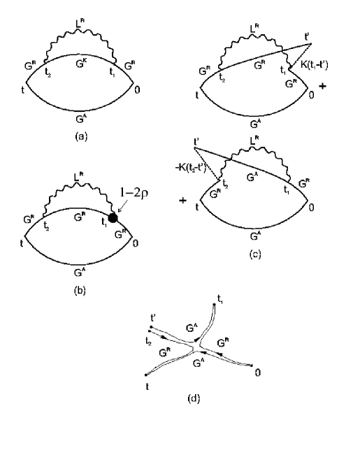
FIG. 3.: The first order diagrams which contain the Keldysh function $G^{K}$ and $\tanh\frac{\epsilon-\omega}{2T}$. (a) Initial diagram. (b) $G^{K}$ is written in the form (A16). (c) $G^{K}$ is written in the form (A14). Two diagrams appear. The second diagram $G^{R}G^{A}G^{R}G^{A}$ contains Hikami boxes. Here we have defined $K(t)=\frac{-iT}{\sinh(\pi Tt)}$. (d) The classical paths which correspond to the second diagram of Fig. 3(c). Such paths violate causality and, hence, do not appear in the path integral.

B

In this Appendix we will present some details of the derivation of eqs. (67-76). Let us first consider the contribution of the self-energy diagrams of Fig. 2a,b and consider only the terms in (A32) which contain the function $I(t,\mathchoice{{\hbox{\boldmath$\displaystyle r$}}}{{\hbox{\boldmath$\textstyle r$}}}{{\hbox{\boldmath$\scriptstyle r$}}}{{\hbox{\boldmath$\scriptscriptstyle r$}}})$, or $\coth(\omega/2T)$. Substituting eqs. (63-65) into these terms of (A32) we find:

$$\delta\sigma_{\alpha\beta}^{\rm coth,se} = -\left[\sum\limits_{\lambda_{1}..\lambda_{4}}\frac{e^{2}}{2}\int\frac{d\mathchoice{{\hbox{\boldmath$\displaystyle r$}}}{{\hbox{\boldmath$\textstyle r$}}}{{\hbox{\boldmath$\scriptstyle r$}}}{{\hbox{\boldmath$\scriptscriptstyle r$}}}_{1}d\mathchoice{{\hbox{\boldmath$\displaystyle r$}}}{{\hbox{\boldmath$\textstyle r$}}}{{\hbox{\boldmath$\scriptstyle r$}}}{{\hbox{\boldmath$\scriptscriptstyle r$}}}_{2}d\mathchoice{{\hbox{\boldmath$\displaystyle r$}}}{{\hbox{\boldmath$\textstyle r$}}}{{\hbox{\boldmath$\scriptstyle r$}}}{{\hbox{\boldmath$\scriptscriptstyle r$}}}_{3}d\mathchoice{{\hbox{\boldmath$\displaystyle r$}}}{{\hbox{\boldmath$\textstyle r$}}}{{\hbox{\boldmath$\scriptstyle r$}}}{{\hbox{\boldmath$\scriptscriptstyle r$}}}_{4}}{{\cal V}}\int\limits_{0}^{\infty}dt_{1}\int\limits_{0}^{t_{1}}dt_{2}\int\limits_{0}^{t_{2}}dt_{3}\right.$$ (B3)

$$\left\{\frac{1}{2}\left(\frac{d}{d\xi_{\lambda_{1}}}\tanh\frac{\xi_{\lambda_{1}}}{2T}\right)\hat{j}_{\alpha}\psi_{\lambda_{1}}(\mathchoice{{\hbox{\boldmath$\displaystyle r$}}}{{\hbox{\boldmath$\textstyle r$}}}{{\hbox{\boldmath$\scriptstyle r$}}}{{\hbox{\boldmath$\scriptscriptstyle r$}}}_{1})\psi^{*}_{\lambda_{1}}(\mathchoice{{\hbox{\boldmath$\displaystyle r$}}}{{\hbox{\boldmath$\textstyle r$}}}{{\hbox{\boldmath$\scriptstyle r$}}}{{\hbox{\boldmath$\scriptscriptstyle r$}}}_{2})e^{-i\xi_{\lambda_{1}}t_{1}}\hat{j}_{\beta}\psi_{\lambda_{2}}(\mathchoice{{\hbox{\boldmath$\displaystyle r$}}}{{\hbox{\boldmath$\textstyle r$}}}{{\hbox{\boldmath$\scriptstyle r$}}}{{\hbox{\boldmath$\scriptscriptstyle r$}}}_{2})\psi^{*}_{\lambda_{2}}(\mathchoice{{\hbox{\boldmath$\displaystyle r$}}}{{\hbox{\boldmath$\textstyle r$}}}{{\hbox{\boldmath$\scriptstyle r$}}}{{\hbox{\boldmath$\scriptscriptstyle r$}}}_{3})e^{i\xi_{\lambda_{2}}t_{3}}\right.$$

$$\left.\left.\big{[}I(t_{2}-t_{3},\mathchoice{{\hbox{\boldmath$\displaystyle r$}}}{{\hbox{\boldmath$\textstyle r$}}}{{\hbox{\boldmath$\scriptstyle r$}}}{{\hbox{\boldmath$\scriptscriptstyle r$}}}_{3}-\mathchoice{{\hbox{\boldmath$\displaystyle r$}}}{{\hbox{\boldmath$\textstyle r$}}}{{\hbox{\boldmath$\scriptstyle r$}}}{{\hbox{\boldmath$\scriptscriptstyle r$}}}_{4})\psi_{\lambda_{3}}(\mathchoice{{\hbox{\boldmath$\displaystyle r$}}}{{\hbox{\boldmath$\textstyle r$}}}{{\hbox{\boldmath$\scriptstyle r$}}}{{\hbox{\boldmath$\scriptscriptstyle r$}}}_{3})\psi^{*}_{\lambda_{3}}(\mathchoice{{\hbox{\boldmath$\displaystyle r$}}}{{\hbox{\boldmath$\textstyle r$}}}{{\hbox{\boldmath$\scriptstyle r$}}}{{\hbox{\boldmath$\scriptscriptstyle r$}}}_{4})e^{i\xi_{\lambda_{3}}(t_{2}-t_{3})}\big{]}\psi_{\lambda_{4}}(\mathchoice{{\hbox{\boldmath$\displaystyle r$}}}{{\hbox{\boldmath$\textstyle r$}}}{{\hbox{\boldmath$\scriptstyle r$}}}{{\hbox{\boldmath$\scriptscriptstyle r$}}}_{4})\psi^{*}_{\lambda_{4}}(\mathchoice{{\hbox{\boldmath$\displaystyle r$}}}{{\hbox{\boldmath$\textstyle r$}}}{{\hbox{\boldmath$\scriptstyle r$}}}{{\hbox{\boldmath$\scriptscriptstyle r$}}}_{1})e^{i\xi_{\lambda_{4}}(t_{1}-t_{2})}+\alpha\leftrightarrow\beta\right\}+{\rm c.c.}\right]$$

This complicated expression can be rewritten in a simpler form if we introduce the matrix elements

$$I^{\lambda_{1}\lambda_{3};\lambda_{3}\lambda_{2}}(t) = \int d\mathchoice{{\hbox{\boldmath$\displaystyle r$}}}{{\hbox{\boldmath$\textstyle r$}}}{{\hbox{\boldmath$\scriptstyle r$}}}{{\hbox{\boldmath$\scriptscriptstyle r$}}}_{1}d\mathchoice{{\hbox{\boldmath$\displaystyle r$}}}{{\hbox{\boldmath$\textstyle r$}}}{{\hbox{\boldmath$\scriptstyle r$}}}{{\hbox{\boldmath$\scriptscriptstyle r$}}}_{2}\psi^{*}_{\lambda_{1}}(\mathchoice{{\hbox{\boldmath$\displaystyle r$}}}{{\hbox{\boldmath$\textstyle r$}}}{{\hbox{\boldmath$\scriptstyle r$}}}{{\hbox{\boldmath$\scriptscriptstyle r$}}}_{1})\psi_{\lambda_{3}}(\mathchoice{{\hbox{\boldmath$\displaystyle r$}}}{{\hbox{\boldmath$\textstyle r$}}}{{\hbox{\boldmath$\scriptstyle r$}}}{{\hbox{\boldmath$\scriptscriptstyle r$}}}_{1})I(t,\mathchoice{{\hbox{\boldmath$\displaystyle r$}}}{{\hbox{\boldmath$\textstyle r$}}}{{\hbox{\boldmath$\scriptstyle r$}}}{{\hbox{\boldmath$\scriptscriptstyle r$}}}_{1}-\mathchoice{{\hbox{\boldmath$\displaystyle r$}}}{{\hbox{\boldmath$\textstyle r$}}}{{\hbox{\boldmath$\scriptstyle r$}}}{{\hbox{\boldmath$\scriptscriptstyle r$}}}_{2})\psi^{*}_{\lambda_{3}}(\mathchoice{{\hbox{\boldmath$\displaystyle r$}}}{{\hbox{\boldmath$\textstyle r$}}}{{\hbox{\boldmath$\scriptstyle r$}}}{{\hbox{\boldmath$\scriptscriptstyle r$}}}_{2})\psi_{\lambda_{2}}(\mathchoice{{\hbox{\boldmath$\displaystyle r$}}}{{\hbox{\boldmath$\textstyle r$}}}{{\hbox{\boldmath$\scriptstyle r$}}}{{\hbox{\boldmath$\scriptscriptstyle r$}}}_{2})$$ (B4)

and $j^{\lambda_{1}\lambda_{2}}_{\alpha}$ (68). Then we get

$$\delta\sigma_{\alpha\beta}^{\rm coth,se} = -\frac{e^{2}}{2{\cal V}}\sum\limits_{\lambda_{1}..\lambda_{4}}\int\limits_{0}^{\infty}dt_{1}\int\limits_{0}^{t_{1}}dt_{2}\int\limits_{0}^{t_{2}}dt_{3}\left(\frac{d}{d\xi_{\lambda_{1}}}\tanh\frac{\xi_{\lambda_{1}}}{2T}\right)\left(j^{\lambda_{4}\lambda_{1}}_{\alpha}j^{\lambda_{1}\lambda_{2}}_{\beta}+j^{\lambda_{4}\lambda_{1}}_{\beta}j^{\lambda_{1}\lambda_{2}}_{\alpha}\right)I^{\lambda_{2}\lambda_{3};\lambda_{3}\lambda_{4}}(t_{2}-t_{3})$$ (B6)

$$\cos\left(-\xi_{\lambda_{1}}t_{1}+\xi_{\lambda_{2}}t_{3}+\xi_{\lambda_{3}}(t_{2}-t_{3})+\xi_{\lambda_{4}}(t_{1}-t_{2})\right).$$

Analogously, one can find the contribution of the remaining terms in (A32) containing the function $R(t,\mathchoice{{\hbox{\boldmath$\displaystyle r$}}}{{\hbox{\boldmath$\textstyle r$}}}{{\hbox{\boldmath$\scriptstyle r$}}}{{\hbox{\boldmath$\scriptscriptstyle r$}}})$, or $\tanh(\xi_{\lambda}/2T)$:

$$\delta\sigma_{\alpha\beta}^{\rm tanh,se} = -\frac{e^{2}}{4{\cal V}}\sum\limits_{\lambda_{1}..\lambda_{4}}\int\limits_{0}^{\infty}dt_{1}\int\limits_{0}^{t_{1}}dt_{2}\int\limits_{0}^{t_{2}}dt_{3}\left(\frac{d}{d\xi_{\lambda_{1}}}\tanh\frac{\xi_{\lambda_{1}}}{2T}\right)\left(j^{\lambda_{4}\lambda_{1}}_{\alpha}j^{\lambda_{1}\lambda_{2}}_{\beta}+j^{\lambda_{4}\lambda_{1}}_{\beta}j^{\lambda_{1}\lambda_{2}}_{\alpha}\right)R^{\lambda_{2}\lambda_{3};\lambda_{3}\lambda_{4}}(t_{2}-t_{3})$$ (B8)

$$\tanh\frac{\xi_{\lambda_{3}}}{2T}\;\;\sin\left(-\xi_{\lambda_{1}}t_{1}+\xi_{\lambda_{2}}t_{3}+\xi_{\lambda_{3}}(t_{2}-t_{3})+\xi_{\lambda_{4}}(t_{1}-t_{2})\right).$$

Now we rewrite the functions $I^{\lambda_{2}\lambda_{3};\lambda_{3}\lambda_{4}}(t_{2}-t_{3})$ and $R^{\lambda_{2}\lambda_{3};\lambda_{3}\lambda_{4}}(t_{2}-t_{3})$ as follows:

$$I^{\lambda_{2}\lambda_{3};\lambda_{3}\lambda_{4}}(t_{2}-t_{3})=\int\frac{d\omega}{2\pi}\frac{d^{3}k}{(2\pi)^{3}}\text{Im}\left(\frac{-4\pi}{k^{2}\epsilon(\omega,k)}\right)\coth\frac{\omega}{2T}\left\langle\lambda_{2}\right|e^{i\mathchoice{{\hbox{\boldmath$\displaystyle kr$}}}{{\hbox{\boldmath$\textstyle kr$}}}{{\hbox{\boldmath$\scriptstyle kr$}}}{{\hbox{\boldmath$\scriptscriptstyle kr$}}}}\left|\lambda_{3}\right\rangle\left\langle\lambda_{3}\right|e^{-i\mathchoice{{\hbox{\boldmath$\displaystyle kr$}}}{{\hbox{\boldmath$\textstyle kr$}}}{{\hbox{\boldmath$\scriptstyle kr$}}}{{\hbox{\boldmath$\scriptscriptstyle kr$}}}}\left|\lambda_{4}\right\rangle\cos(\omega(t_{2}-t_{3})),$$ (B9)

$$R^{\lambda_{2}\lambda_{3};\lambda_{3}\lambda_{4}}(t_{2}-t_{3})=\int\frac{d\omega}{2\pi}\frac{d^{3}k}{(2\pi)^{3}}\frac{4\pi}{k^{2}\epsilon(\omega,k)}\left\langle\lambda_{2}\right|e^{i\mathchoice{{\hbox{\boldmath$\displaystyle kr$}}}{{\hbox{\boldmath$\textstyle kr$}}}{{\hbox{\boldmath$\scriptstyle kr$}}}{{\hbox{\boldmath$\scriptscriptstyle kr$}}}}\left|\lambda_{3}\right\rangle\left\langle\lambda_{3}\right|e^{-i\mathchoice{{\hbox{\boldmath$\displaystyle kr$}}}{{\hbox{\boldmath$\textstyle kr$}}}{{\hbox{\boldmath$\scriptstyle kr$}}}{{\hbox{\boldmath$\scriptscriptstyle kr$}}}}\left|\lambda_{4}\right\rangle e^{-i\omega(t_{2}-t_{3})}.$$ (B10)

Now let us express the kernel $R$ (B10) in terms of the imaginary part of the inverse dielectric susceptibility. Firstly we write $1/\epsilon=1-(1-1/\epsilon)$. The function $1-1/\epsilon$ is regular in the upper half-plane of $\omega$ and it tends to zero if $\omega\rightarrow\infty$. Therefore for $t_{2}>t_{3}$ one has

$$\int\frac{d\omega}{2\pi}\left(\frac{1}{\epsilon(\omega,k)}-1\right)e^{i\omega(t_{2}-t_{3})}\equiv 0.$$

Since in the integral (B8) the time $t_{2}$ indeed exceeds $t_{3}$, we can replace $e^{-i\omega(t_{2}-t_{3})}$ by $e^{-i\omega(t_{2}-t_{3})}-e^{i\omega(t_{2}-t_{3})}$ in the integral (B10). Then we arrive at the following result:

$$R^{\lambda_{2}\lambda_{3};\lambda_{3}\lambda_{4}}(t_{2}-t_{3}) = \delta(t_{2}-t_{3}-0)\left\langle\lambda_{2}\right|_{\mathchoice{{\hbox{\boldmath$\displaystyle r$}}}{{\hbox{\boldmath$\textstyle r$}}}{{\hbox{\boldmath$\scriptstyle r$}}}{{\hbox{\boldmath$\scriptscriptstyle r$}}}_{1}}\left\langle\lambda_{3}\right|_{\mathchoice{{\hbox{\boldmath$\displaystyle r$}}}{{\hbox{\boldmath$\textstyle r$}}}{{\hbox{\boldmath$\scriptstyle r$}}}{{\hbox{\boldmath$\scriptscriptstyle r$}}}_{2}}\frac{1}{|\mathchoice{{\hbox{\boldmath$\displaystyle r$}}}{{\hbox{\boldmath$\textstyle r$}}}{{\hbox{\boldmath$\scriptstyle r$}}}{{\hbox{\boldmath$\scriptscriptstyle r$}}}_{1}-\mathchoice{{\hbox{\boldmath$\displaystyle r$}}}{{\hbox{\boldmath$\textstyle r$}}}{{\hbox{\boldmath$\scriptstyle r$}}}{{\hbox{\boldmath$\scriptscriptstyle r$}}}_{2}|}\left|\lambda_{3}\right\rangle_{\mathchoice{{\hbox{\boldmath$\displaystyle r$}}}{{\hbox{\boldmath$\textstyle r$}}}{{\hbox{\boldmath$\scriptstyle r$}}}{{\hbox{\boldmath$\scriptscriptstyle r$}}}_{1}}\left|\lambda_{4}\right\rangle_{\mathchoice{{\hbox{\boldmath$\displaystyle r$}}}{{\hbox{\boldmath$\textstyle r$}}}{{\hbox{\boldmath$\scriptstyle r$}}}{{\hbox{\boldmath$\scriptscriptstyle r$}}}_{2}}-$$ (B12)

$$-2\int\frac{d\omega}{2\pi}\frac{d^{3}k}{(2\pi)^{3}}\text{Im}\left(\frac{-4\pi}{k^{2}\epsilon(\omega,k)}\right)\left\langle\lambda_{2}\right|e^{i\mathchoice{{\hbox{\boldmath$\displaystyle kr$}}}{{\hbox{\boldmath$\textstyle kr$}}}{{\hbox{\boldmath$\scriptstyle kr$}}}{{\hbox{\boldmath$\scriptscriptstyle kr$}}}}\left|\lambda_{3}\right\rangle\left\langle\lambda_{3}\right|e^{-i\mathchoice{{\hbox{\boldmath$\displaystyle kr$}}}{{\hbox{\boldmath$\textstyle kr$}}}{{\hbox{\boldmath$\scriptstyle kr$}}}{{\hbox{\boldmath$\scriptscriptstyle kr$}}}}\left|\lambda_{4}\right\rangle\sin(\omega(t_{2}-t_{3})).$$

The correction to the conductivity due to the self-energy diagrams can now be written as

$$\delta\sigma^{\rm se}_{\alpha\beta} = \delta\sigma_{\alpha\beta}^{C}-\frac{e^{2}}{2{\cal{V}}}\int\limits_{0}^{+\infty}dt_{1}\sum\limits_{\lambda_{1}..\lambda_{4}}\left(\frac{d}{d\xi_{\lambda_{1}}}\tanh\frac{\xi_{\lambda_{1}}}{2T}\right)\left(j_{\alpha}^{\lambda_{4}\lambda_{1}}j_{\beta}^{\lambda_{1}\lambda_{2}}+j_{\beta}^{\lambda_{4}\lambda_{1}}j_{\alpha}^{\lambda_{1}\lambda_{2}}\right)\times$$ (B14)

$$\ \times\int\frac{d\omega}{2\pi}\frac{d^{3}k}{(2\pi)^{3}}\;\;\text{Im}\left(\frac{-4\pi}{k^{2}\epsilon(\omega,k)}\right)\left\langle\lambda_{2}\right|e^{i\mathchoice{{\hbox{\boldmath$\displaystyle kr$}}}{{\hbox{\boldmath$\textstyle kr$}}}{{\hbox{\boldmath$\scriptstyle kr$}}}{{\hbox{\boldmath$\scriptscriptstyle kr$}}}}\left|\lambda_{3}\right\rangle\left\langle\lambda_{3}\right|e^{-i\mathchoice{{\hbox{\boldmath$\displaystyle kr$}}}{{\hbox{\boldmath$\textstyle kr$}}}{{\hbox{\boldmath$\scriptstyle kr$}}}{{\hbox{\boldmath$\scriptscriptstyle kr$}}}}\left|\lambda_{4}\right\rangle\left[\coth\frac{\omega}{2T}+\tanh\frac{\xi_{\lambda_{3}}}{2T}\right]F(t_{1},\omega,\xi_{\lambda_{1}}..\xi_{\lambda_{4}}),$$

where $\delta\sigma_{\alpha\beta}^{C}$ (73) is the correction due to the non-screened Coulomb interaction and the function $F$ is defined in eq. (69).

Now let us make use of the Drude approximation for the dielectric susceptibility of a disordered metal

$$\epsilon(\omega,k)=\frac{4\pi\sigma}{-i\omega+Dk^{2}}.$$

In this case it is convenient to introduce the matrix elements $M^{\lambda_{2}\lambda_{3};\lambda_{3}\lambda_{4}}$ as defined in eq. (68). Combining the above expressions we immediately arrive at the final result for the first order correction to the conductivity from self-energy diagrams of Fig. 2a,b (67), (69).

The conductivity correction from the vertex diagrams of Fig. 2c,d is evaluated analogously. After a straightforward algebra we obtain

$$\delta\sigma_{\alpha\beta}^{\rm coth,vert} = \frac{e^{2}}{2{\cal V}}\sum\limits_{\lambda_{1}..\lambda_{4}}\int\limits_{0}^{\infty}dt_{1}\int\limits_{0}^{t_{1}}dt_{2}\int\limits_{0}^{t_{2}}dt_{3}\left(\frac{d}{d\xi_{\lambda_{1}}}\tanh\frac{\xi_{\lambda_{1}}}{2T}\right)\left(j_{\alpha}^{\lambda_{2}\lambda_{3}}j_{\beta}^{\lambda_{1}\lambda_{4}}+j_{\beta}^{\lambda_{2}\lambda_{3}}j_{\alpha}^{\lambda_{1}\lambda_{4}}\right)I^{\lambda_{3}\lambda_{1};\lambda_{4}\lambda_{2}}(t_{2}-t_{3})$$ (B16)

$$\cos(-\xi_{\lambda_{3}}(t_{1}-t_{3})-\xi_{\lambda_{1}}t_{3}+\xi_{\lambda_{4}}t_{2}+\xi_{\lambda_{2}}(t_{1}-t_{2})),$$

$$\delta\sigma_{\alpha\beta}^{\rm tanh,vert} = -\frac{e^{2}}{4{\cal V}}\sum\limits_{\lambda_{1}..\lambda_{4}}\int\limits_{0}^{\infty}dt_{1}\int\limits_{0}^{t_{1}}dt_{2}\int\limits_{0}^{t_{2}}dt_{3}\left(\frac{d}{d\xi_{\lambda_{1}}}\tanh\frac{\xi_{\lambda_{1}}}{2T}\right)\left(j_{\alpha}^{\lambda_{2}\lambda_{3}}j_{\beta}^{\lambda_{1}\lambda_{4}}+j_{\beta}^{\lambda_{2}\lambda_{3}}j_{\alpha}^{\lambda_{1}\lambda_{4}}\right)R^{\lambda_{3}\lambda_{1};\lambda_{4}\lambda_{2}}(t_{2}-t_{3})$$ (B18)

$$\tanh\frac{\xi_{\lambda_{3}}}{2T}\sin(-\xi_{\lambda_{3}}(t_{1}-t_{3})-\xi_{\lambda_{1}}t_{3}+\xi_{\lambda_{2}}t_{2}+\xi_{\lambda_{4}}(t_{1}-t_{2})).$$

Introducing again the matrix elements (68) and combining (B16) and (B18) we arrive at the result (75), (76).

C

In this Appendix we will analyze the expressions for the weak localization correction to the conductance obtained by AAG in the limit $\tau_{H}\ll\tau_{\varphi}$ perturbatively in the interaction. This additional analysis is necessary because the final results for the most interesting low temperature limit $T\tau_{H}\lesssim 1$ were not presented in Ref. [13]. For the sake of definiteness we will consider only the 1d case which is sufficient for our purposes.

AAG split the total expression for the weak localization correction to the conductance into two terms:

$$\delta\sigma_{WL}^{AAG}=\delta\sigma_{\rm deph}^{AAG}+\delta\sigma_{CWL}^{AAG},$$ (C1)

where – according to Ref. [13] – the first term describes dephasing while the second term accounts for the renormalization due to interaction and has nothing to do with dephasing. Below we will demonstrate that such a separation of the weak localization correction into “dephasing” and “interaction” terms is not possible even within the perturbation theory employed by AAG.

Let us consider the first term in (C1) which was defined in eqs. (4.5), (4.6) of Ref. [13] and has the form

$$\delta\sigma_{\rm deph}^{AAG}=\frac{\sigma}{\pi{\cal V}}\int\frac{dQdq}{(2\pi)^{2}}\int\frac{d\omega}{2\pi}\left(\frac{\omega}{2T}\right)^{2}\frac{1}{\sinh^{2}\frac{\omega}{2T}}\left(\frac{4Te^{2}}{\sigma_{1}q^{2}}\right)\left(\left[{\cal C}(Q,0)\right]^{2}{\cal C}(Q+q,\omega)-\left|{\cal C}(Q,\omega)\right|^{2}{\cal C}(Q+q,0)\right),$$ (C2)

where the Cooperon and the diffuson are defined as follows:

$${\cal C}(\omega,q)=\frac{1}{-i\omega+Dq^{2}+1/\tau_{H}},\;\;\;{\cal D}(\omega,q)=\frac{1}{-i\omega+Dq^{2}}.$$ (C3)

The integrals over $Q$ and $q$ in (C2) can be evaluated exactly and we find

$$\delta\sigma_{\rm deph}^{AAG} = \frac{\sigma}{2\pi{\cal V}^{2}}\frac{\tau_{H}^{2}}{D}{\rm Im}\int\frac{d\omega}{2\pi}\frac{\omega}{2T\sinh^{2}\frac{\omega}{2T}}\left[\frac{i\omega\tau_{H}}{2\sqrt{1+i\omega\tau_{H}}(\sqrt{1+i\omega\tau_{H}}-1)^{2}}\left(\frac{1}{\sqrt{1+i\omega\tau_{H}}-1}-\frac{1}{2}\right)-\right.$$ (C5)

$$\left.-\frac{4}{(i\omega\tau_{H})^{2}}-\frac{(\sqrt{1+i\omega\tau_{H}}-1)^{2}}{2(i\omega\tau_{H})^{2}\sqrt{1+i\omega\tau_{H}}}\right]$$

Making use of this equation we get

$$\delta\sigma_{\rm deph}^{AAG} \simeq \frac{e^{2}}{\pi}\frac{e^{2}}{\sigma_{1}}\left\{\frac{DT\tau_{H}^{2}}{4}\left(1+\zeta(1/2)\sqrt{\frac{2}{\pi T\tau_{H}}}\right)+\frac{5}{8}\frac{\zeta(3/2)}{\pi}\sqrt{\frac{D^{2}\tau_{H}}{2\pi T}}\right\},\;\;\;T\tau_{H}\gg 1,$$ (C6)

$$\delta\sigma_{\rm deph}^{AAG} \simeq \frac{e^{2}}{\pi}\frac{e^{2}}{\sigma_{1}}\frac{\pi^{4}}{30}D\tau_{H}(T\tau_{H})^{4},\;\;\;T\tau_{H}\ll 1$$ (C7)

In the limit $T\tau_{H}\gg 1$ the expression (C7) practically coincides with the analogous expression obtained in Ref. [13] (see eq. (4.11) of that paper) with the only difference in a numerical coefficient in front of the last term in the first equation (C7) ($5/8$ in our calculation and $1/2$ in Ref. [13]). In the opposite limit $T\tau_{H}\ll 1$ the expression (C2) was not evaluated by AAG at all.

Now let us consider the second contribution (C1) which was denoted by AAG as a cross term of weak localization and interaction. According to Ref. [13] this term has the following structure (see eq. (5.23) of that paper)

$$\delta\sigma^{\rm CWL}=\frac{\sigma}{2\pi{\cal V}^{2}}{\rm Im}\int\frac{d\omega}{2\pi}\left[\frac{d}{d\omega}\left(\omega\coth\frac{\omega}{2T}\right)\right]\left[I_{1}(\omega)+2I_{2}(\omega)-4I_{3}(\omega)+4I_{4}(\omega)+I_{5}(\omega)+8I_{6}(\omega)\right],$$ (C8)

where the terms in the square brackets are defined in eqs. (5.25) of [13]:

$$I_{1}(\omega) = \int\frac{dQdq}{(2\pi)^{2}}\frac{1}{Dq^{2}}\left\{{\cal C}^{2}(0,Q)\left[\frac{{\cal C}(-\omega,Q+q)}{{\cal D}(-\omega,q)}-1\right]+\left[{\cal C}(-\omega,Q)-{\cal C}(0,Q)\right]{\cal D}(-\omega,q)+2{\cal C}(-\omega,Q+q){\cal C}(0,Q)\right\},$$ (C9)

$$I_{2}(\omega) = \int\frac{dQdq}{(2\pi)^{2}}\frac{q}{Dq^{2}}\frac{\partial}{\partial q}{\cal C}(-\omega,Q+q){\cal C}(0,Q),$$ (C10)

$$I_{3}(\omega) = \int\frac{dQdq}{(2\pi)^{2}}{\cal D}(-\omega,q){\cal C}(-\omega,Q+q){\cal C}(0,Q),$$ (C11)

$$I_{4}(\omega) = \int\frac{dQdq}{(2\pi)^{2}}\frac{Q}{q}{\cal D}(-\omega,q){\cal C}(0,Q-q){\cal C}(-\omega,Q),$$ (C12)

$$I_{5}(\omega) = \int\frac{dQdq}{(2\pi)^{2}}{\cal D}(-\omega,q){\cal C}^{2}(-\omega,Q),$$ (C13)

$$I_{6}(\omega) = \int\frac{dQdq}{(2\pi)^{2}}Dq^{2}{\cal D}^{3}(-\omega,q){\cal C}(-\omega,Q).$$ (C14)

These integrals can also be evaluated exactly and we arrive at the following results:

$$I_{1}(\omega) = \frac{\tau_{H}^{2}}{4D}\frac{\sqrt{1+i\omega\tau_{H}}-1}{(i\omega\tau_{H})^{3/2}\sqrt{1+i\omega\tau_{H}}},$$ (C15)

$$I_{2}(\omega) = \frac{\tau_{H}^{2}}{4D}\frac{1}{(i\omega\tau_{H})^{2}}\left(2-\sqrt{1+i\omega\tau_{H}}-\frac{1}{\sqrt{1+i\omega\tau_{H}}}\right),$$ (C16)

$$I_{3}(\omega) = \frac{\tau_{H}^{2}}{8D}\left(\frac{1}{\sqrt{i\omega\tau_{H}}\sqrt{1+i\omega\tau_{H}}}-\frac{\sqrt{1+i\omega\tau_{H}}-1}{i\omega\tau_{H}\sqrt{1+i\omega\tau_{H}}}\right),$$ (C17)

$$I_{4}(\omega) = \frac{\tau_{H}^{2}}{4D}\left(\frac{\sqrt{1+i\omega\tau_{H}}-1}{(i\omega\tau_{H})^{2}}+\frac{\sqrt{1+i\omega\tau_{H}}-1}{2(i\omega\tau_{H})^{3/2}}-\frac{1}{2(i\omega\tau_{H})}\right),$$ (C18)

$$I_{5}(\omega) = \frac{\tau_{H}^{2}}{8D}\frac{1}{\sqrt{i\omega\tau_{H}}(1+i\omega\tau_{H})^{3/2}},$$ (C19)

$$I_{6}(\omega) = \frac{\tau_{H}^{2}}{32D}\frac{1}{(i\omega\tau_{H})^{3/2}\sqrt{1+i\omega\tau_{H}}}.$$ (C20)

Let us compare these exact expressions with those obtained in Ref. [13]. Unfortunately AAG calculated the integrals approximately only in the limit of high frequencies $\omega\tau_{H}\gg 1$. In this limit they found

$$I_{1}^{AAG}(\omega) \simeq \frac{\tau_{H}^{2}}{4D}\left(\frac{1}{(i\omega\tau_{H})^{3/2}}-\frac{1}{(i\omega\tau_{H})^{2}}\right),$$ (C21)

$$I_{2}^{AAG}(\omega) \simeq \frac{\tau_{H}^{2}}{4D}\left(-\frac{1}{(i\omega\tau_{H})^{3/2}}+\frac{2}{(i\omega\tau_{H})^{2}}\right),$$ (C22)

$$I_{3}^{AAG}(\omega) \simeq \frac{\tau_{H}^{2}}{4D}\left(\frac{1}{2(i\omega\tau_{H})^{3/2}}-\frac{1}{4(i\omega\tau_{H})^{2}}\right),$$ (C23)

$$I_{4}^{AAG}(\omega) \simeq \frac{\tau_{H}^{2}}{8D}\left(\frac{1}{(i\omega\tau_{H})^{3/2}}-\frac{3}{2(i\omega\tau_{H})^{2}}\right),$$ (C24)

$$I_{5}^{AAG}(\omega) \simeq \frac{\tau_{H}^{2}}{8D}\frac{1}{(i\omega\tau_{H})^{2}},$$ (C25)

$$I_{6}^{AAG}(\omega) \simeq \frac{\tau_{H}^{2}}{64D}\frac{1}{(i\omega\tau_{H})^{2}}.$$ (C26)

In order to find a numerical coefficient in front of the term $\sim 1/(i\omega\tau_{H})^{2}$ in the expression for $I_{4}^{AAG}$ (C26) we exactly evaluated the integral

$$\int_{0}^{\infty}dxdydz\frac{y\exp(-x-y)}{(y+z)\sqrt{xy+xz+yz}}=\frac{\pi}{2}$$

(see eq. (5.25d) of Ref. [13]) which was not calculated by AAG.

The high frequency asymptotics of the functions $I_{1},I_{2},I_{3},I_{4}$ and $I_{5}$ coincide with the results (C26), while the asymptotic results for $I_{6}$ derived from the exact expressions (C20) in the limit $\omega\tau_{H}\gg 1$ takes the form

$$I_{6}(\omega)\simeq\frac{\tau_{H}^{2}}{32D}\frac{1}{(i\omega\tau_{H})^{2}}.$$

We observe a difference in the numerical prefactor in the exact expression and in the term $I_{6}^{AAG}$ (C26) found in Ref. [13].

A much more important problem is, however, not in this numerical discrepancy, but rather in the fact that AAG evaluated the integrals only in the limit $\omega\tau_{H}\gg 1$ and did not study the behavior of the integrals (C14) at lower frequencies $\omega\tau_{H}\lesssim 1$ at all. Note that the low frequency behavior of these integrals is crucially important because it determines the dependence of the weak localization correction on $\tau_{H}$ at sufficiently low temperatures $T\tau_{H}\lesssim 1$. [Let us remind the reader that here we are discussing only the limit of strong magnetic fields [13] $\tau_{H}\ll\tau_{\varphi}$ beyond which any perturbative (in the interaction) calculation of the weak localization correction is meaningless. Clearly, in this limit the condition $T\tau_{H}\lesssim 1$ is compatible with the condition $T\tau_{\varphi}\gg 1$.]

It is easy to observe from (C20) that at low frequencies the integrals $I_{1}$, $I_{3}$, $I_{4}$, $I_{5}$ behave as $\propto 1/\sqrt{i\omega\tau_{H}}$, the integral $I_{2}$ tends to a constant at $\omega\to 0$, while the integral $I_{6}$ behaves as $I_{6}\propto 1/(i\omega\tau_{H})^{3/2}$. It implies that the contribution of the integrals $I_{1}$,..,$I_{5}$ to the conductivity correction (C8) does not diverge as temperature goes to zero but stays finite for any finite $\tau_{H}$ even at $T=0$. The contribution of the integral $I_{6}$ diverges as $1/\sqrt{T}$ for low $T$. Note, that in the high frequency limit (C26) all the integrals show the same asymptotic behavior, and one could naively conclude that all these integrals are of the same origin. In reality, however, only (a part of) the integral $I_{6}$ can be interpreted as the effect of interaction on the weak localization, while all other terms actually contribute to dephasing, at least for not very high temperatures $T\tau_{H}\lesssim 1$.

Let us split the function $I_{6}$ (C20) into two terms which give respectively divergent and convergent contributions to the integral of $I_{6}(\omega)$ over $\omega$ at low frequencies

$$I_{6}(\omega)=\frac{\tau_{H}^{2}}{32D}\frac{1}{(i\omega\tau_{H})^{3/2}}-\frac{\tau_{H}^{2}}{32D}\frac{\sqrt{1+i\omega\tau_{H}}-1}{(i\omega\tau_{H})^{3/2}\sqrt{1+i\omega\tau_{H}}}$$ (C27)

We will now treat only the first (divergent) term in this equation, while the second (convergent) term will be added to the integrals $I_{1}$,..,$I_{5}$. The divergent term yields the following contribution:

$$\delta\sigma_{\rm CWL} = \frac{\sigma}{2\pi\nu^{2}}{\rm Im}\int\frac{d\omega}{2\pi}\left[\frac{d}{d\omega}\left(\omega\coth\frac{\omega}{2T}\right)\right]8\frac{\tau_{H}^{2}}{32D}\frac{1}{(i\omega\tau_{H})^{3/2}}$$ (C28)

$$= -\frac{e^{2}}{2\pi}\sqrt{\frac{D}{2\pi T}}\left(\frac{3\zeta(3/2)}{2}\right)\frac{e^{2}}{\pi\sigma}\sqrt{D\tau_{H}}=-\frac{1}{2}\delta\sigma_{C}(T)\frac{\delta\sigma_{WL}}{\sigma},$$ (C29)

where

$$\delta\sigma_{C}(T)=-\frac{e^{2}}{\pi}\sqrt{\frac{D}{2\pi T}}\left(\frac{3\zeta(3/2)}{2}\right)$$ (C30)

is the interaction correction to the conductivity, and

$$\delta\sigma_{WL}=-\frac{e^{2}}{\pi}\sqrt{D\tau_{H}}$$ (C31)

is the weak localization correction. Within the validity range of the perturbation theory in the interaction, the equation (C29) is valid in the whole temperature interval from $T\tau_{H}\ll 1$ to $T\tau_{H}\gg 1$. The physical origin of the correction (C29) is quite transparent. Indeed, the interaction term (C30) contains the photon propagator ${\cal L}^{R}\propto 1/\sigma$. If one replaces the total conductivity by the sum of the Drude conductivity and the weak localization correction, one will immediately observe that in the first order in $\delta\sigma_{WL}$ the interaction correction will be transformed as $\delta\sigma_{C}\to\delta\sigma_{C}(1-\delta\sigma_{WL}/\sigma)$. Thus we arrive at (C29).

This simple consideration clarifies the origin of the correction (C29). It can be interpreted as the effect of weak localization on the interaction correction. The same conclusion follows if one considers the diagrams contributing to the integral $I_{6}$. They are just the diagrams which yield the interaction correction multiplied by the weak localization correction to the photon propagator. In other words, the contribution (C29) originates from the second term in the right-hand side of eq. (5.22) in Ref. [13], while all the remaining contributions come from the first term, i.e. from the unrenormalized photon propagator. Collecting all these contributions we express the final result [13] for $\delta\sigma^{AAG}_{CWL}$ (C8) as a sum of two terms

$$\delta\sigma_{CWL}^{AAG}=\delta\sigma_{CWL}+\delta\sigma^{??},$$ (C32)

where $\delta\sigma_{CWL}$ is defined in (C29) and

$$\delta\sigma^{??}=\left\{\begin{array}[]{ll}\frac{e^{2}}{\pi}\frac{e^{2}}{\sigma_{1}}\left\{\frac{3}{2\pi}D\tau_{H}+{\cal O}\left(D\tau_{H}\sqrt{T\tau_{H}}\right)\right\},&T\tau_{H}\ll 1\\ \frac{3}{2}\frac{e^{2}}{\pi}\sqrt{\frac{D}{2\pi T}}\left(\frac{3\zeta(3/2)}{2}\right)\frac{e^{2}}{\pi}\frac{\sqrt{D\tau_{H}}}{\sigma_{1}},&T\tau_{H}\gg 1.\end{array}\right.$$ (C33)

can be derived from the eq. (C8) combined with (C20).

We observe that for $T\tau_{H}\lesssim 1$ the contribution proportional to $\tau_{H}$ dominates and determines the behavior of $\delta\sigma^{??}$ as a function of $\tau_{H}$. This contribution cannot be interpreted as an interaction correction since it grows faster than $\sqrt{\tau_{H}}$ with increasing $\tau_{H}$. For quasi-1d systems all contributions to the conductance growing faster than $\sqrt{\tau_{H}}$ should be interpreted as dephasing terms (see also our discussion in Section 2). Thus – although the correct and complete description of the interaction-induced decoherence cannot be obtained from the perturbation theory in the interaction – the conclusion about the existence of temperature-independent dephasing in disordered conductors at low $T$ (determined by the range of frequencies $\omega>T$) follows already from the perturbative calculation [13]! This is in contrast with the qualitative arguments about the absence of zero-temperature dephasing presented in the same paper.

It also follows from the above consideration that the suggested by AAG splitting of the weak localization correction into two terms (C1) can hardly be justified in both limits $T\tau_{H}\gg 1$ and $T\tau_{H}\ll 1$ even within the framework of their perturbation calculation [13]. Indeed, for $T\tau_{H}\gg 1$ the total expression for the weak localization correction $\delta\sigma_{CWL}^{AAG}$ derived by AAG and defined here in eqs. (C1), (C2), (C8) and (C14) can be expressed as a series expansion in $1/\sqrt{T\tau_{H}}$:

$$\delta\sigma_{WL}^{AAG}\simeq\frac{e^{2}}{\pi}\frac{e^{2}}{\sigma_{1}}\frac{DT\tau_{H}^{2}}{4}\left(1+{\cal O}\left(\sqrt{\frac{1}{T\tau_{H}}}\right)\right).$$ (C34)

In this limit $\delta\sigma_{CWL}^{AAG}$ is vanishingly small (it contributes only to the next after the subleading term in (C34) and can be safely disregarded. Moreover, for $T\tau_{H}\gg 1$ exactly the same term $\sim\delta\sigma_{CWL}^{AAG}\propto\sqrt{\tau_{H}/T}$ (with a slightly different numerical prefactor) is contained in the expression for $\delta\sigma_{\rm deph}^{AAG}$ (C7). Also due to this fact there are no reasons to distinguish the term $\delta\sigma_{CWL}^{AAG}$ from the remaining contribution to $\delta\sigma_{WL}^{AAG}$ in the above limit.

For $T\tau_{H}\sim 1$ both terms in (C1) are of the same order, and therefore their separation is not possible. Finally, in the limit $T\tau_{H}\ll 1$ the result for $\delta\sigma_{WL}^{AAG}$ reads

$$\delta\sigma_{WL}^{AAG}=\delta\sigma_{CWL}+\frac{e^{2}}{\pi}\frac{e^{2}}{\sigma_{1}}\frac{3D\tau_{H}}{2\pi}(1+{\cal O}(\sqrt{T\tau_{H}})).$$ (C35)

The origin of the term $\delta\sigma_{CWL}\propto\sqrt{\tau_{H}/T}$ (C29) was clarified above. It does not describe dephasing and it is purely a matter of convention whether to include this term into the perturbative weak localization or interaction corrections. The second term in (C35) is represented as a series expansion in powers of $\sqrt{T\tau_{H}}$, it describes dephasing and remains finite even at $T=0$. We emphasize again that in the limit $T\tau_{H}\ll 1$ the leading “dephasing-type” contribution to the perturbative weak localization correction comes from $\delta\sigma_{CWL}^{AAG}$ and not from the “dephasing” term [13] $\delta\sigma_{\rm deph}^{\rm AAG}$ which only contributes to the higher order terms ($\sim(T\tau_{H})^{4}$) of the expansion of $\delta\sigma_{WL}^{AAG}$ in powers of $T\tau_{H}$ (cf. eq. (C7)). Terms of the same order are also contained in the expression for $\delta\sigma_{CWL}^{AAG}$. Thus the splitting (C1) is not justified also in the limit $T\tau_{H}\ll 1$.

D

For reference purposes we present some rigorous expressions obtained within the exactly solvable Caldeira-Leggett model [8] for a quantum particle with coordinate $x$ interacting with an infinite bath of oscillators. The time evolution of the density matrix of such a particle is defined by eq. (1) and the kernel $J$ is given by the following path integral:

$$J(t,x_{1f},x_{2f},x_{1i},x_{2i})=\int\limits^{x_{1f}}_{x_{1i}}{\cal D}x_{1}(t)\int\limits^{x_{2f}}_{x_{2i}}{\cal D}x_{2}(t)\exp\left(iS_{0}[x_{1}(t)]-iS_{0}[x_{2}(t)]-iS_{R}[x_{1}(t),x_{2}(t)]-S_{I}[x_{1}(t),x_{2}(t)]\right),$$ (D1)

where $S_{0}[x]=\int\limits_{0}^{t}dt^{\prime}\;\;(m\dot{x}^{2}/2)$ is the action of a free particle. The interaction part of the action has the following form

$$S_{R}[x_{1},x_{2}] = \int\limits_{0}^{t}dt_{1}\int\limits_{0}^{t_{1}}dt_{2}\left\{\alpha_{R}(t_{1}-t_{2})x_{1}(t_{1})x_{1}(t_{2})-\alpha_{R}(t_{1}-t_{2})x_{2}(t_{1})x_{2}(t_{2})+\right.$$ (D3)

$$\left.\alpha_{R}(t_{1}-t_{2})x_{1}(t_{1})x_{2}(t_{2})-\alpha_{R}(t_{1}-t_{2})x_{2}(t_{1})x_{1}(t_{2})\right\}+\frac{1}{2}\left(\int\frac{d\omega}{2\pi}\;\frac{2I(\omega)}{\omega}\right)\int\limits_{0}^{t}dt^{\prime}[x^{2}_{1}(t^{\prime})-x^{2}_{2}(t^{\prime})],$$

$$S_{I}[x_{1},x_{2}] = \int\limits_{0}^{t}dt_{1}\int\limits_{0}^{t_{1}}dt_{2}\left\{\alpha_{I}(t_{1}-t_{2})x_{1}(t_{1})x_{1}(t_{2})+\alpha_{I}(t_{1}-t_{2})x_{2}(t_{1})x_{2}(t_{2})-\right.$$ (D5)

$$\left.\alpha_{I}(t_{1}-t_{2})x_{1}(t_{1})x_{2}(t_{2})-\alpha_{I}(t_{1}-t_{2})x_{2}(t_{1})x_{1}(t_{2})\right\}.$$

The kernels $\alpha_{I}$ and $\alpha_{R}$ are given by the following integrals:

$$\alpha_{R}(t) = -i\int\frac{d\omega}{2\pi}\;I(\omega)e^{-i\omega t},$$ (D6)

$$\alpha_{I}(t) = \int\frac{d\omega}{2\pi}\;I(\omega)\coth\frac{\omega}{2T}e^{-i\omega t},$$ (D7)

where $I(\omega)$ is the spectral density of the oscillators. This function can be arbitrary, but we will consider here only the case of Ohmic dissipation, $I(\omega)=\eta\omega\theta(\omega_{c}-|\omega|)$, with $\omega_{c}$ being the high cutoff frequency. This spectrum is the most relevant in view of comparison to the disordered metal. The last term in the action $S_{R}$ (D3) compensates potential renormalization caused by the interaction and maintains the translational invariance of the system.

The kernel $J$ (D1) can be found exactly as the integrals over the coordinates are Gaussian. One finds (see e.g. [8, 9])

$$J(t,x_{1f},x_{2f},x_{1i},x_{2i}) = \frac{\eta}{2\pi(1-e^{-\gamma t})}\exp\left[i\eta\frac{x^{+}_{f}x^{-}_{f}+e^{\gamma t}x^{+}_{i}x^{-}_{i}-e^{\gamma t}x^{+}_{f}x^{-}_{i}-x^{+}_{i}x^{-}_{f}}{e^{\gamma t}-1}-\right.$$ (D9)

$$\left.-\eta\big{\{}g_{1}(t){x^{-}_{i}}^{2}+g_{2}(t)(x^{-}_{f}-x^{-}_{i})^{2}+g_{3}(t)x^{-}_{i}(x^{-}_{f}-x^{-}_{i})\big{\}}\right],$$

where

$$g_{1}(t) = \frac{1}{2}\int\limits_{0}^{t}ds\int\limits_{0}^{t}ds^{\prime}\;\;G(s-s^{\prime})\simeq Tt+\ln\frac{1-e^{-2\pi Tt}}{2\pi(T/\omega_{c})},\;\;\;t\gg\omega_{c}^{-1}$$ (D10)

$$g_{2}(t) = \frac{1}{2}\int\limits_{0}^{t}ds\int\limits_{0}^{t}ds^{\prime}\;\;\frac{(e^{\gamma s}-1)G(s-s^{\prime})(e^{\gamma s^{\prime}}-1)}{(e^{\gamma t}-1)^{2}}$$ (D11)

$$g_{3}(t) = \int\limits_{0}^{t}ds\int\limits_{0}^{t}ds^{\prime}\;\;\frac{G(s-s^{\prime})(e^{\gamma s^{\prime}}-1)}{(e^{\gamma t}-1)},$$ (D12)

and

$$G(t)=\int\limits_{-\omega_{c}}^{\omega_{c}}\frac{d\omega}{2\pi}\;\;\omega\coth\frac{\omega}{2T}e^{-i\omega t}=-\frac{1}{\pi}\left(\frac{\pi T}{\sinh(\pi Tt)}\right)^{2}.$$ (D13)

E

As it was already pointed out, the authors of several recent papers [15, 16, 17] arrived at conclusions different from ours [5, 6, 7] and, moreover, argued that our approach [6] is not correct. On top of the standard arguments (which have been already discussed in the bulk of this paper) the authors [15, 16, 17] suggested various additional reasons which could invalidate our analysis. In view of that we feel it will be appropriate to address the arguments presented in the above papers. We believe that this Appendix can be useful for the reader who would like to follow the details of the discussion around the problem of quantum decoherence at low temperatures.

Cohen and Imry (CI) [15] proceeded within the Feynman-Vernon influence functional formalism and found that the interference of any pair of time reversed paths is suppressed due to interaction with an effective environment even at $T=0$. This result (eq. (12) of Ref. [15]) implies a nonzero decoherence rate at $T=0$ and is consistent with our results [5, 6, 7] as well with the results of other authors [28, 29] obtained within the framework of the CL model. However, CI argued that the saddle-point approximation they used “cannot be trusted” at low temperatures, and the $T$-independent contribution to the dephasing rate “should be omitted”. The CI’s arguments in favor of this conclusion follow the line of reasoning according to which a particle with the energy $\sim T$ cannot excite environmental modes with energies exceeding $T$.

The arguments [15] can not be accepted. Indeed, if CI do not trust the saddle-point approximation which gives nonzero dephasing down to $T=0$, this could only imply that one should analyze the role of fluctuations around the saddle points. The contribution of non-saddle-point paths may only yield further suppression of quantum coherence simply because the relevant saddle points provide the (local) minimum for the action. The imaginary part of the effective action is positive $S_{I}>0$ for all paths except for pairs of exactly equal paths in which case $S_{I}\equiv 0$. [The latter paths do not contribute to the dephasing rate.] Thus the saddle point approximation may only underestimate the dephasing rate.

We can add that in our problem the applicability of the saddle point approximation cannot depend on temperature. This is particularly clear in the weak interaction limit. In this case the saddle point paths are determined only by the “noninteracting” parts of the action which do not depend on temperature at all. The “interacting” contribution can then be treated perturbatively in the exponent (cf. e.g. Sec. 5C), and this is a completely legitimate procedure controlled by a small parameter $1/p_{F}l\ll 1$ in the case of disordered metals. At sufficiently high $T$ this procedure yields the AAK’s result [2]. If one accepts the saddle-point approximation at higher $T$, one should accept it also at lower $T$: the saddle point paths are the same and the “interacting” contribution to the exponent may only decrease with decreasing $T$. The saddle point approximation which treats the interaction term perturbatively in the exponent (and thus yields energy conservation on the saddle point paths) is well known and was frequently used for the Feynman-Vernon influence functionals, see e.g. Refs. [34, 35].

CI [15] also mentioned the simple perturbative results which – according to them – yield zero decoherence rate at $T=0$. As it was already explained above, (i) the problem is essentially nonperturbative and no information about the dephasing time $\tau_{\varphi}$ can be extracted from perturbation theory in the interaction (Sec. 2) and (ii) at low temperatures the golden rule approximation yields incorrect results even for perturbative terms (Sec. 4B). Eqs. (14), (15) of Ref. [15] can be obtained from the equation above eq. (14) of the same paper only within the golden rule approximation (83). Exact calculation leads to an additional term (cf. eqs. (86) and (152)) which survives even at $T=0$ and diverges at large times. Unfortunately this term is missing in eq. (14) of Ref. [15].

The same term is missing also in eq. (1) of the paper by Imry, Fukuyama and Schwab (IFS) [17]. Already this fact as well as our analysis of Sec. 2 invalidates the “proof that zero-point motion does not dephase” presented by IFS. Again, their eqs. (1), (2) are obtained within the same golden rule approximation. Since IFS allow for a general form of the interaction matrix elements, it should be legitimate to take ones e.g. for the CL model and to substitute them into eq. (1) of Ref. [17]. Then one would immediately arrive at the conclusion that no decoherence occurs in the CL model at $T=0$. Thus the proof of Ref. [17] explicitly contradicts to the results obtained within the exactly solvable Caldeira-Leggett model.

IFS also argued that dephasing cannot occur at $T\to 0$ in equilibrium because “in that limit neither the electron nor the environment has any energy to exchange”. It is well known, however, that the energy of a subsystem (an electron in our case) interacting with other subsystem (other electrons) is not conserved due to interaction. The energy exchange between different subsystems of a closed system is, of course, possible even at $T=0$. In the presence of interaction with any other quantum degrees of freedom an electron can be described only by the density matrix [30] and is (obviously) not in its noninteracting ground state. Therefore it always has energy to exchange. The same is true for the environment: it is well known [31] that an imaginary part of the dielectric susceptibility for a large system Im$\epsilon$ does not vanish even at $T=0$, thus implying the possibility of energy exchange. The above argument [17] disregards the interaction term in the Hamiltonian, and this is again nothing but the golden rule approximation (see also Appendix B of Ref. [14] for further discussion of this point). Due to interaction the ground state energy of the total system is different from (in our case larger than) the sum of energies of its noninteracting parts, and the energy exchange is always possible.

IFS also pointed out that our results [5, 6] are “in disagreement with experiments” of Ref. [36]. The experimental results for the dephasing time $\tau_{\varphi}$ were reported only in one (the second) out of three papers under Ref. [36]. In this experiment it was found that at sufficiently low $T$ (below $\sim 1\div 3$ K) “the dependence $L_{\varphi}(T)$ is flattened out”. The comparison between our results for $\tau_{\varphi}$ and the experimental findings of the second Ref. [36] was carried out in Ref. [7]. An excellent agreement was revealed for all three samples studied in the second paper [36], see Fig. 3 of Ref. [7]. Therefore, it remains unclear which of our results was meant by the authors [17] to be in disagreement with experiments [36].

Since this point was not clarified by IFS we can try to conjecture that they actually interpreted our conclusion [5] that Coulomb interaction in weakly disordered quasi-1d metallic (many channel) conductors (described within the standard Drude model) precludes the Thouless crossover into an insulating state as contradicting to a rapid growth of the wire resistance with decreasing temperature detected in Ref. [36] below $T\sim 1$ K. If so, we can only point out that the above conclusion does not contradict to the experimental data but only to their interpretation in terms of the Thouless crossover adopted in Ref. [36]. The wire conductivity can be represented as a sum of the Drude term $\sigma_{1}$, the interaction correction $\delta\sigma_{int}(T)$ and the weak localization correction $\delta\sigma_{WL}(T,H)$:

$$\sigma_{1}+\delta\sigma_{int}(T)+\delta\sigma_{WL}(T,H).$$

Our analysis [5, 6] demonstrates that the last of these three terms saturates at low $T$, and this is in agreement with the observations reported in the second Ref. [36]. However the total resistance may well keep increasing at even lower $T$ because of the interaction term $\delta\sigma_{int}(T)$. This scenario indeed precludes the “noninteracting” Thouless crossover, but not the crossover into an insulating state due to interaction (e.g. of the Coulomb blockade type). Since in Refs. [5, 6] we did not address the term $\delta\sigma_{int}(T)$ at all, one can hardly argue about any contradiction between our results and the experimental data [36].

Finally let us turn to the paper by Vavilov and Ambegaokar [16]. These authors did not employ the “orthodox” golden rule approximation [15, 17, 18] but rather attempted to analyze the problem by means of a high temperature expansion. They also presented a critical analysis of our paper [6] (see Appendix C of Ref. [16]).

VA questioned the validity of our procedure which amounts to deriving a dephasing time $\tau_{\varphi}$ only from the terms in our expression for the effective action [6] which dominate at sufficiently long times. According to VA the dropped terms might be important at times $t\sim\tau_{\varphi}$ (where $S_{I}(\tau_{\varphi})\sim 1$) and due to that the result for $\tau_{\varphi}$ could be different from ours [6]. Even without making any calculation one can realize that the contribution of these dropped terms, if important, could only make the dephasing time shorter than that found in our paper [6]. Indeed, if one assumes that taking all terms into account one would obtain a longer dephasing time $\tau_{\varphi}^{\prime}\gg\tau_{\varphi}$, one would immediately arrive at a contradiction with the fact (acknowledged by VA) that the dropped terms are unimportant at times $t\gg\tau_{\varphi}$: at least at times $t\sim\tau_{\varphi}^{\prime}$ (and, hence, at $t\gg\tau_{\varphi}$) these dropped terms should still be significant. Since this is not the case, by neglecting the above terms one actually gets an upper bound for $\tau_{\varphi}$. This is in contrast with the VA’s claim that $\tau_{\varphi}$ is parametrically longer than that found in our paper [6] at low $T$.

The analysis presented in Sec. 3A of this paper fully confirms our previous results [6]. All terms of our effective action [6] were explicitly taken into account in eq. (24). Additional terms in the exponent (see eqs. (30), (35)-(41)) indeed appear, but (i) they lead to further suppression of quantum coherence and (ii) for all times $t\gtrsim\tau_{\varphi}$ they are small as compared to the leading order terms which we already considered before [6].

The problem with “unphysical divergences” discussed in the beginning of Appendix C of Ref. [16] does not exist in our analysis either. This can be observed already from the footnote 32 before eq. (76) of Ref. [6]: the actual low frequency cutoff in this equation is at $\omega\sim 1/t$, see also eqs. (46), (47) of Ref. [7]. This cutoff is not imposed by hand, but rather follows from the fact that the integral over $\omega$ in eq. (76) of Ref. [6] and related formulas is just the long time approximation of the sum over discrete Fourier frequencies $\omega_{n}=2\pi n/t$. [The cutoff at $\sim 1/\tau_{\varphi}$ was used e.g. by AAK [2] and in many other papers, we have followed this approximate and physically correct procedure in eq. (76) of Ref. [6] just in order to illustrate the similarity of the low frequency contribution to $\tau_{\varphi}$ found in Refs. [6] and [2].] The absence of any “unphysical divergences” in the exact expression (24) is also completely transparent. It is hard to understand why VA believe that our results cannot be compared to those obtained within the Caldeira-Leggett model. A close similarity between both problems is obvious from our analysis presented in Sec. 5.

Another problem of VA with our analysis has to do with the factor $(1-2n({\mathchoice{{\hbox{\boldmath$\displaystyle p$}}}{{\hbox{\boldmath$\textstyle p$}}}{{\hbox{\boldmath$\scriptstyle p$}}}{{\hbox{\boldmath$\scriptscriptstyle p$}}}},{\mathchoice{{\hbox{\boldmath$\displaystyle r$}}}{{\hbox{\boldmath$\textstyle r$}}}{{\hbox{\boldmath$\scriptstyle r$}}}{{\hbox{\boldmath$\scriptscriptstyle r$}}}}))$ which appears in the real part $S_{R}$ of our effective action (see eq. (A43)). VA stated that in Ref.[6] we “neglected the time dependence of the momentum”. This is not true. The electron momentum changes its direction after each scattering event, an this fact is explicitly taken into account in Ref. [6] where the classical electron trajectories in a disordered potential were considered. No momentum conservation was imposed in our analysis, rather the electron energy conservation on these trajectories was used. This approximation is fully justified, since the saddle point paths are determined by the “noninteracting” terms in the effective action while “interacting” terms are treated as a perturbation in the exponent. For these saddle point paths the factor $(1-2n({\mathchoice{{\hbox{\boldmath$\displaystyle p$}}}{{\hbox{\boldmath$\textstyle p$}}}{{\hbox{\boldmath$\scriptstyle p$}}}{{\hbox{\boldmath$\scriptscriptstyle p$}}}},{\mathchoice{{\hbox{\boldmath$\displaystyle r$}}}{{\hbox{\boldmath$\textstyle r$}}}{{\hbox{\boldmath$\scriptstyle r$}}}{{\hbox{\boldmath$\scriptscriptstyle r$}}}}))$ (and not ${\mathchoice{{\hbox{\boldmath$\displaystyle p$}}}{{\hbox{\boldmath$\textstyle p$}}}{{\hbox{\boldmath$\scriptstyle p$}}}{{\hbox{\boldmath$\scriptscriptstyle p$}}}}(t)$) does not depend on time. It is not quite clear why VA suggest to consider odd functions of time $n({\mathchoice{{\hbox{\boldmath$\displaystyle p$}}}{{\hbox{\boldmath$\textstyle p$}}}{{\hbox{\boldmath$\scriptstyle p$}}}{{\hbox{\boldmath$\scriptscriptstyle p$}}}}(t))$. Such functions do not contribute to the exponent at all. It is also not clear in which context the observation [16] that for an odd function of time $n({\mathchoice{{\hbox{\boldmath$\displaystyle p$}}}{{\hbox{\boldmath$\textstyle p$}}}{{\hbox{\boldmath$\scriptstyle p$}}}{{\hbox{\boldmath$\scriptscriptstyle p$}}}}(t))$ the real part of the action $S_{R}$ is of the same order as $S_{I}$ (taken at $T=0$) could be important: there is no way how the term $iS_{R}$ can cancel $S_{I}$ for real and nonzero $S_{R}$ and $S_{I}$. The contribution of the trajectories with nonzero $S_{R}$ to the path integral may only be suppressed further due to the presence of the oscillating term $\exp(-iS_{R})$.

Trying to justify their arguments VA presented several equations (eqs. (C12-C15) of Ref. [16]) which are somewhat reminiscent to ones obtained e.g. in Sec. 4 of this paper. For instance, the combination “coth+tanh” appears in eq. (C15) of Ref. [16] in a correct form (80) rather than in the form (79) used by some other authors. Unfortunately VA did not evaluate their eq. (C15) but just concluded “we see that the contribution of high frequencies is exponentially suppressed”. In Sec. 4B we have demonstrated just the opposite: the high frequency contribution is not exponentially suppressed even at $T\to 0$ and, moreover, it leads to the presence of diverging terms already in the first order in the interaction (cf. eq. (86)). Exactly the same terms are contained in eq. (C15) of Ref. [16] and, hence, the above statement [16] is explicitly incorrect. In Ref. [16] we also failed to find a proof of even stronger VA’s statement that one can “observe the same type of cancellation of high frequency contributions to the conductivity in any order of perturbation theory”.

Having observed that none of our results [6] suffers from the VA’s “critique” let us come to the analysis of the calculation [16]. In order to understand the problems with this calculation we have to start from another paper of the same authors [37]. VA acknowledged that the paper [37] “is simply wrong, because it treats the phase as a single particle and looses the physics associated with the exclusion principle”. We cannot agree with the second part of this statement. In our opinion, it was a good idea of Ref. [37] to apply the Caldeira-Leggett model in order to qualitatively understand the experimental results [1]. It is not the absence of the exclusion principle in this model, it is the calculation of Ref. [37] which is problematic. In particular, we mention that according to Ref. [37] the real part of the action $S_{R}$ is responsible for the low temperature saturation of $\tau_{\varphi}$ whereas the contribution of its imaginary part $S_{I}$ is not important at $T\to 0$. A correct calculation demonstrates the opposite: both in the CL model and in the case of a disordered metal the term $S_{I}$ is important, while the term $S_{R}$ does not contribute to the exponent (and thus to the dephasing time) at all. The term $S_{R}$ vanishes on the saddle-point trajectories both with and without the exclusion principle, i.e. the latter does not play any crucial role in the problem in question.

Revising their earlier paper, VA applied the same method of calculating the path integral as one employed in Ref. [37]. Should the term $S_{R}$ be kept in the exponent, the result [37] would follow again. In order to avoid that VA expanded the exponent to the first order in $S_{R}$ and in the “quantum” part of $S_{I}$ and made use of the perturbation theory developed in Ref. [13]. Several comments are in order.

1. Even if the perturbative calculations [16] of the weak localization correction in the high temperature limit were correct, the correct dephasing time $\tau_{\varphi}$ could not be extracted from these calculations. The reason for that is exactly the same as for the perturbative calculation [13]: the $T$-independent linear in time perturbative contributions coming from the Taylor expansion of the exponent and the pre-exponent exactly cancel each other in the first order. As it was explained in Sec. 2 the problem of finding the dephasing time $\tau_{\varphi}$ is essentially nonperturbative and, hence, the method [16] should fail already at the point where the exponent was (partially) expanded in powers of the interaction.

2. The perturbative analysis [13] cannot simply be repeated for the situation considered by VA because the initial (non-perturbed) propagators depend on the classical part of the fluctuating field. This implies that the Fourier transformation in time cannot easily be performed, and the whole calculation should be redone from the very beginning.

3. In order to obtain the “classical” part of the weak localization correction VA used a minimization procedure, the meaning of which remains unclear. Indeed, let us rewrite eq. (92) of Ref. [16] for the weak localization correction in the presence of interaction (for the sake of transparency we keep the notations adopted in the above paper)

   $$\Delta\sigma_{wl}=\Delta\sigma_{wl}^{(0)}+\Delta\sigma_{deph}+\Delta\sigma_{deph}^{\prime},$$ (E1)

   As compared to eq. (92) of Ref. [16], in (E1) we omitted the last (smallest) term $\Delta\sigma_{cwl}$ which is unimportant for our discussion. According to VA the first term $\Delta\sigma_{wl}^{(0)}$ comes from the “diagram without electron-electron interaction with finite dephasing rate $\gamma$”. This should imply that the rate $\gamma$ in Ref. [16] is not due to the electron-electron interaction but rather due to some other dephasing mechanism. E.g. in the presence of the magnetic field one has $\gamma\equiv 1/\tau_{H}$ and eq. (93) of Ref. [16] for $\Delta\sigma_{wl}^{(0)}$ is equivalent to our eq. (8) or to the first equation (4.2b) of Ref. [13]. The second term $\Delta\sigma_{deph}$ is equivalent to the first term in eq. (4.13a) of Ref. [13] (or to the first term in eq. (135) of the present paper)) provided one assumes $\gamma\equiv 1/\tau_{H}$. This term already originates from the electron-electron interaction (classical Nyquist noise), but again the decoherence rate $\gamma$ is not related to this interaction but rather is due to some other mechanism. We also note that the term $\Delta\sigma_{deph}$ written in the form of eq. (96) of Ref. [16] makes sense only if it is small $\Delta\sigma_{deph}\ll\Delta\sigma_{wl}^{(0)}$.

   The next step of the authors [16] is not easy to understand. They minimize the sum of the first two terms in (E1) with respect to the dephasing rate $\gamma$ and in this way they “self-consistently” derive $\gamma\sim 1/\tau_{\varphi}^{AAK}\propto T^{2/3}$. Unfortunately VA did not clarify (i) why the result (E1) should be minimized with respect to $\gamma$ and (ii) why the rate $\gamma$ depends now on the electron-electron interaction though initially it was assumed that $\gamma$ is not related to the electron-electron interaction at all. [Actually VA minimized only the two first terms in (E1). This implies that these terms can be of the same order in contradiction to the inequality $\Delta\sigma_{deph}\ll\Delta\sigma_{wl}^{(0)}$]. No explanation of the above procedure was given in Ref. [16].

4. VA found a negative “quantum” correction $\Delta\sigma_{deph}^{\prime}$, see e.g. eqs. (88-89) of Ref. [16]. From this result VA concluded that the dephasing rate [2] “is overestimated, and the quantum correction suppresses it”. In other words, according to the authors [16] quantum noise – at least at not very low $T$ – acts “against” the classical noise. No physical reasons supporting this strange result was presented in Ref. [16]. Fortunately there is no need to look for such reasons. It is obvious e.g. from our eq. (35) that the correction to the classical dephasing rate [2] is positive at any relevant temperature, i.e. quantum noise may only enhance the dephasing effect of the classical noise. Below we will demonstrate that no conclusion about both the sign and the value of the quantum correction to the classical dephasing rate can be drawn from the expression for the leading order high temperature correction $\Delta\sigma_{deph}^{\prime}$.

5. VA’s procedure can easily be tested with the aid of the results derived in the present paper. Since the authors [16] assume “that the electron-electron interaction is the only mechanism of decoherence” and consider only the high temperature limit, in our formulas of Sec. 2-4 we can put $1/\tau_{H}=0$ and keep only the term

   $$f_{1cl}(t)=\frac{4}{3}\frac{e^{2}}{\sigma_{1}}\sqrt{\frac{D}{\pi}}Tt^{3/2}$$ (E2)

   in the exponent of (6) expanding this exponent to the first order in $f_{1}(t)-f_{1cl}(t)$. We also expand the pre-exponent $A_{1}(t)$ to the first order in the interaction $A_{1}(t)\simeq A_{1}^{(0)}(t)+A_{1}^{(1)}(t)$, where $A_{1}^{(0)}(t)=1/(2\sqrt{\pi Dt})$. This procedure should exactly correspond to the high temperature expansion of Ref. [16]. Then for the weak localization correction (E1) (which we now denote as $\delta\sigma_{WL}$) we will obtain

   $$\delta\sigma_{WL}=-\frac{e^{2}\sqrt{D}}{\pi^{3/2}}\int\limits_{0}^{+\infty}\frac{dt}{\sqrt{t}}e^{-f_{1cl}(t)}+\frac{e^{2}\sqrt{D}}{\pi^{3/2}}\int\limits_{0}^{+\infty}\frac{dt}{\sqrt{t}}\left(f_{1}(t)-f_{1cl}(t)-\frac{A_{1}^{(1)}(t)}{A_{1}^{(0)}(t)}\right)e^{-f_{1cl}(t)}.$$ (E3)

   Here the first integral determines the “classical” part of the weak localization correction while the second integral gives the “quantum” correction. Both integrals can easily be evaluated. Combining eqs. (35), (106) and (134) (the last equation allows to evaluate the term $A_{1}^{(1)}(t)/A_{1}^{(0)}(t)$) and keeping only the leading corrections from the high temperature expansion we obtain

   $$f_{1}(t)-f_{1cl}(t)-\frac{A_{1}^{(1)}(t)}{A_{1}^{(0)}(t)}\simeq\frac{\zeta(1/2)}{\sqrt{2}}\frac{e^{2}}{\sigma_{1}}\sqrt{\frac{D}{\pi}}t\sqrt{T}.$$ (E4)

   As before, the $T$-independent linear in time terms contained in $f_{1}(t)$ (35) and in $A_{1}^{(1)}(t)/A_{1}^{(0)}(t)$ exactly cancel each other. This cancellation illustrates again why the correct dephasing time at low $T$ as well as the leading order high temperature correction to the classical dephasing rate cannot be recovered by means of a high temperature expansion for the conductance. From (E2)-(E4) we find

   $$\delta\sigma_{WL}\simeq-\left(\frac{2e^{4}\sigma_{1}D}{9\pi^{4}T}\right)^{1/3}\Gamma(1/3)+\frac{\zeta(1/2)}{(2\pi)^{3/2}}\frac{e^{2}\sqrt{D}}{\sqrt{T}}.$$ (E5)

We conclude that the procedure developed by VA in Ref. [16] does not provide correct information about the interaction-induced dephasing in disordered conductors.

REFERENCES

- [1] P. Mohanty, E.M.Q. Jariwala, and R.A. Webb, Phys. Rev. Lett. 78, 3366 (1997); Fortsch. Phys. 46, 779 (1998).
- [2] B.L. Altshuler, A.G. Aronov, and D.E. Khmelnitskii, J. Phys. C 15, 7367 (1982).
- [3] B.L. Altshuler and A.G. Aronov, in Electron-Electron Interactions in Disordered Systems, edited by A.L. Efros and M. Pollak (North-Holland, Amsterdam, 1985), p.1.
- [4] P. Mohanty and R.A. Webb, Phys. Rev. B 55 13452 (1997).
- [5] D.S. Golubev and A.D. Zaikin, Phys. Rev. Lett. 81, 1074 (1998).
- [6] D.S. Golubev and A.D. Zaikin, Phys. Rev. B 59, 9195 (1999).
- [7] D.S. Golubev and A.D. Zaikin, Physica B 225, 164 (1998).
- [8] A.O. Caldeira and A.J. Leggett, Physica A 121, 587 (1983); 130, 374 (1985).
- [9] U. Weiss, Quantum Dissipative Systems (World Scientific, Singapore, second enlarged edition, 1999).
- [10] B.L. Altshuler, M.E. Gershenzon, and A.L. Aleiner, Physica E 3, 58 (1998).
- [11] I.L. Aleiner, B.L. Altshuler, and M.E. Gershenzon, Phys. Rev. Lett. 82, 3190 (1999).
- [12] For our reply to Ref. [11] see D.S. Golubev and A.D. Zaikin, Phys. Rev. Lett. 82, 3191 (1999).
- [13] I.L. Aleiner, B.L. Altshuler, and M.E. Gershenzon, cond-mat/9808053; Waves in Random Media, 9, 201 (1999).
- [14] For our reply to Ref. [13] see D.S. Golubev and A.D. Zaikin, cond-mat/9811185.
- [15] D. Cohen and Y. Imry, cond-mat/9807038 v2.
- [16] M. Vavilov and V. Ambegaokar, cond-mat/9902127.
- [17] Y. Imry, H. Fukuyama, and P. Schwab, cond-mat/9903017; Europhys. Lett. 47, 608 (1999).
- [18] R. Raimondi, P. Schwab, and C. Castellani, cond-mat/9903146.
- [19] Yu. V. Nazarov, Sov. Phys. JETP 68, 561 (1989); M.H. Devoret et al. Phys. Rev. Lett. 64, 1824 (1990); S.M. Girvin et al., ibid. 64, 1565 (1990).
- [20] G. Schön and A.D. Zaikin, Phys. Rep. 198, 237 (1990).
- [21] A.N. Cleland, J.M. Schmidt, and J. Clarke, Phys. Rev. B. 45, 2950 (1992); L.S.Kuzmin et al., Phys. Rev. Lett. 67, 1161 (1991); D.B. Haviland et al., Europhys. Lett. 16, 103 (1991); P. Joyez, D. Esteve, and M.H. Devoret, Phys. Rev. Lett. 80, 1956 (1998).
- [22] D.S. Golubev and A.D. Zaikin, cond-mat/9907497; to appear in: Quantum Physics at Mesoscopic Scale eds. D.C. Glattli, M. Sanquer and J. Tran Thanh Van (Frontieres, 1999).
- [23] R.P. Feynman and F.L. Vernon Jr., Ann. Phys. (NY) 24, 118 (1963).
- [24] R.P. Feynman and A.R. Hibbs, Quantum Mechanics and Path Integrals (McGraw Hill, NY, 1965).
- [25] S. Chakravarty and A. Schmid, Phys. Rep. 140, 193 (1986).
- [26] H. Fukuyama and E. Abrahams, Phys. Rev. B 27, 5976 (1983).
- [27] Ya.M. Blanter, Phys. Rev. B 54, 12807 (1996).
- [28] D. Loss and K. Mullen, Phys. Rev. B 43, 13252 (1991).
- [29] See Chapter 9 of Ref. [9].
- [30] See e.g. L.D. Landau and E.M. Lifshitz, Quantum Mechanics, (Pergamon, Oxford, 1977).
- [31] See e.g. E.M. Lifshitz and L.P. Pitaevskii, Statistical Physics, Vol. 2 (Pergamon, New York, 1980).
- [32] Y. Levinson, cond-mat/9907055.
- [33] S.M. Alamoudi, D. Boyanovsky, and H.J. de Vega, cond-mat/9812029.
- [34] S. Chakravarty, Phys. Rev. Lett. 49, 681 (1982); A.J. Bray and M.A. Moore, Phys. Rev. Lett. 49, 1545 (1982); A. Schmid, Phys. Rev. Lett. 51, 1506 (1983); S.A. Bulgadaev, Pis’ma Zh. Eksp. Teor. Fiz. 39, 264 (1984) [JETP Lett. 39, 315 (1984)]; F. Guinea, V. Hakim, and A. Muramatsu, Phys. Rev. Lett. 54, 263 (1985).
- [35] S. Chakravarty and A.J. Leggett, Phys. Rev. Lett. 53, 5 (1984); A.J. Leggett et al., Rev. Mod. Phys. 59, 1 (1986).
- [36] Yu.B. Khavin, M.E. Gershenzon, and A.L. Bogdanov, Sov. Phys. Uspekhi 168, 200 (1998); Phys. Rev. Lett., 81, 1066 (1998); Phys. Rev. B 58, 8009 (1998).
- [37] M. Vavilov and V. Ambegaokar, cond-mat/9709241.