Dipoles and fractional quantum Hall masses

Abstract

We develop a microscopic formalism to study the fractional quantum Hall plateaus at filling factors $\nu$ away from $1/2\beta$ $\beta$ an integer. The theory is in terms of quasiparticles which carry a charge $e^{\ast}$ equal to $1-2\beta\nu$ times the charge of the electron. The wave functions obtained following our approach are shown to coincide precisely with the form predicted by Jain and this holds independently of the interaction potential. Microscopically this rigidity originates from the fact that two different charges interacting attractively in their lowest Landau levels form a bound state with a universal wave function. From the expressions of the gaps we compute an effective mass which agrees well with the experiments carried at $\nu=1/2$ and $1/4$.

Many fundamental aspects of the fractional quantum Hall effect (FQHE) have resulted from a better understanding of the vicinity of the $\nu=1/2$ filling factor. Jain was able to obtain the most prominent FQHE plateaus by reinterpreting the FQHE as an integer quantum Hall effect (IQHE) for particles which experience a reduced magnetic field [1]. Halperin Lee and Read have predicted that the system behaves in a Fermi liquid way [9] at the filling fraction $\nu=1/2\beta,\ \beta=1,2$. Their theory provides a convincing explanation of the anomaly observed at $\nu=1/2$ (and less strongly at $\nu=1/4$) in the surface acoustic propagation by Willet et al. [3]. Several experiments [4] have seen that slightly away from $\nu=1/2\beta$ the electrons move in circles as if they experience a reduced magnetic field $\Delta B=B-B_{0}$. A phenomenological way to account for these properties is to assume that the relevant excitations, also called composite fermions (CF), carry a fractional charge varying continuously with the filling factor, $e^{\ast}=(1-2\beta\nu)e$. Although such fractional charges have been observed in noise experiments [5], they have not been clearly identified with the CF. We propose here a microscopic derivation of the CF properties in terms of quasiparticles which carry a fractional charge. Each electron is replaced by a quasiparticle and the missing charge is carried by an incompressible charged vacuum.

Another feature of the FQHE is that unlike in the IQHE, the gaps responsible for it are due to the interactions. Here we set mass of the electrons to zero and the CF acquire an effective cyclotron energy due to their interactions. The novelty is to predict microscopically a rigid structure for the wave functions independently of the interacting potential. When the filling fraction gets close to $1/2\beta$ the states connect continuously to the Fermi-liquid states at $\nu=1/2\beta$. The activation gaps are then given by the Landau Level spacing $\Delta=e^{*}\hbar B/m^{*}$ where $m^{*}$ defines the composite-fermions effective mass. The masses we obtain are very sensitive to the parameter $\lambda$ which simulates the effect of the thickness of the sample. A very good agreement with experimental results [7] is obtained when this parameter is of the order of the magnetic length [28].

In order to understand the origin of the effective charge $e^{\ast}$ and how the cyclotron energy results from the repulsive interactions one approach initiated by Read [10] (see also [11, 12, 13, 14]) suggests that the $\nu=1/2$ low energy quasiparticles are dipoles. This picture can be related to the trial wave functions [1, 6, 9] if one notes [9, 11, 17, 16] that the effect of the Lowest Landau Level (LLL) projection inherent to these wave functions is to displace the electrons from their positions in a $\nu=1/2\beta$ bosonic Laughlin wave function. In [11, 15] we developed a theory where the fundamental excitations were these dipoles. We represented one excitation by two opposite charges interacting attractively in a magnetic field [18, 19, 20]. They form a bound state which moves in a straight line and carries a dipole momentum perpendicular to its canonical momentum. When projected into the LLL the eigenfunctions are independent of the attractive potential. They can be expanded on the LLL basis of the particle and hole and the expansion coefficients form a matrix which is the projection of a plane wave into the LLL. To a first approximation the $\nu=1/2\beta$ CF can be described by non interacting dipoles and the wave function studied in [6, 9] is the antisymmetrized product of these projected plane waves.

We follow the same approach to study the CF at filling fractions away from $\nu=1/2\beta$. The main modification is that the electron charge differs from that of the hole. The charge of the hole varies with the magnetic field so that a system of particles with this charge and a density equal to that of the electrons has a constant filling factor equal to $1/2\beta$. The reason for this choice is to construct a bosonic system which remains incompressible as the magnetic field is varied and which defines the vacuum of the CF excitations. In this description the CF is a particle hole excitation where the statistics and the charge of the particle differ from that of the hole. As a consequence the bound state made by the electron and its correlation hole acquires a charge $e^{*}=(1-2\nu)e$ [11, 21, 22]. In the following we use units where $\hbar=c=l=1$, $l=\sqrt{\hbar c/eB}$ is the magnetic length. The product of the charge of the electron and of the hole by the magnetic field $B$ are denoted $q_{a}$ and $q_{b}$. $q_{a}=1$ in our units and $q_{b}=2\beta\nu q_{a}$.

Let us first consider a simple model which contains in essence the main points developed in this letter: A single electron and its correlated hole are coupled by a spring. Their coordinates are $x_{a(b)},y_{a(b)}=\vec{x}_{a(b)}$. In the Landau gauge their dynamics follows the Lagrangian:

$${\it L}=(q_{a}x_{a}\dot{y}_{a}-q_{b}x_{b}\dot{y}_{b})-K/2((x_{a}-x_{b})^{2}+(y_{a}-y_{b})^{2})$$ (1)

where in (1) we have have taken the strong $B$ field limit which enables to neglect the masses of the particles to be neglected. For simplicity we consider here the case $q_{a}>q_{b}$. The momenta of $y_{a}$ and $y_{b}$ are $p_{a}=q_{a}x_{a}$ and $p_{b}=-q_{b}x_{b}$. The Hamiltonian is:

$$H=K/2((p_{a}/q_{a}+p_{b}/q_{b})^{2}+(y_{a}-y_{b})^{2})$$ (2)

Its eigenfunctions are given by:

$$\chi_{P_{Y},n}(y_{a},y_{b})=e^{iP_{Y}(q_{a}y_{a}-q_{b}y_{b})/(q_{a}-q_{b})}e^{-(y_{a}-y_{b})^{2}/(q_{b}^{-1}-q_{a}^{-1})}H_{n}((y_{a}-y_{b})/(q_{b}^{-1}-q_{a}^{-1})^{1/2})$$ (3)

where $P_{Y}$ is the momentum in the $y$ direction and $H_{n}(x)$ are the Hermite polynomials. The $x$ coordinate $X=(q_{a}x_{a}+q_{b}x_{b})/(q_{a}+q_{b})$ and the $y$-momentum $P_{Y}=p_{a}+p_{b}$ are related by $P_{Y}=\langle X\rangle(q_{a}-q_{b})$. This means that the two charges move as a charge $q^{*}=q_{a}-q_{b}$ in the magnetic field. The harmonic oscillator frequency gives the effective mass of the bound state to be: $q_{a}q_{b}/K$. Assuming that the electrons behave as a gas of noninteracting such bound states, at the filling factors of the principal series $\nu=n/{2\beta n+1}$ the effective filling factor of the reduced charge $q^{*}$ is equal to $n$, which explains the occurrence of the FQHE at these fractions. At $\nu=1/2\beta$, $q^{*}=0$, and the Hamiltonian reduces to a free Hamiltonian $H=P^{2}/{2m^{*}}$ so that we expect a Fermi sea to form. The momentum $\vec{P}$ and the relative coordinate are then related by $-P_{X}=q_{a}(y_{a}-y_{b}),\ P_{Y}=q_{a}(x_{a}-x_{b})$ so that the bound state behaves as a neutral dipole with a dipole vector perpendicular and proportional to its momentum. Note that since the strength $K$ of the spring enters the Hamiltonian (2) as a normalization factor the wave function (3) which describes the two charges is independent of $K$.

If we replace the spring by a rotation invariant potential $V(r)$, one can refine the preceding approach to show that the wave function of the bound state is independent of the potential. To see it we need to consider the problem of the particle and the hole interacting in their respective LLL. The orbital of a charge $q$ particle in the $n^{th}\geq 0$ Landau level is denoted $u_{n,t}^{q}$ (simply $u_{t}^{q}$ for $n=0$) where $t$ is the momentum in the $y$ direction:

$$u_{n,t}^{q}(x,y)=e^{ity}H_{n}(\sqrt{q}(x-t/q))e^{-q(x-t/q)^{2}/2}$$ (4)

The wave function for the charge and the hole can be decomposed on a basis of LLL orbitals:

$$\chi_{P_{Y},n}(x_{a},x_{b},y_{a},y_{b})=\sum_{s-t=P_{Y}}\hat{\chi}^{P_{Y},n}_{st}u^{q_{a}}_{s}(x_{a},y_{a})\bar{u}^{q_{b}}_{t}(x_{b},y_{b})$$ (5)

and the coefficients $\hat{\chi}^{P_{Y},n}_{st}$ are obtained by diagonalizing the potential interaction:

$$\sum_{s^{\prime}t^{\prime}}\langle st^{\prime}|V|s^{\prime}t\rangle\hat{\chi}^{P_{Y},n}_{s^{\prime}t^{\prime}}=-\epsilon_{n}^{0}\hat{\chi}^{P_{Y},n}_{st}$$ (6)

The matrix elements $\langle st|V|s^{\prime}t^{\prime}\rangle$ are taken between LLL orbitals of charge $q_{a}$ for $s,s^{\prime}$ and $q_{b}$ for $t,t^{\prime}$. Without loss of generality we restrict ourselves to the zero momentum case $P_{Y}=0$, $(s=t,s^{\prime}=t^{\prime}),$ and we consider a Gaussian potential $V(r)=e^{-r^{2}/{2\mu^{2}}}$. In the large system size limit, the momentum index $s$ becomes continuous and the secular problem (6) rewrites:

$${1\over 1+1/{\mu^{2}q_{b}}}\sqrt{1/q_{b}-1/q_{a}\over\pi(1-\tau^{2})}\int_{-\infty}^{\infty}e^{-(1/q_{b}-1/q_{a})((s^{2}+s^{\prime 2})(1+\tau^{2})/2-2\tau ss^{\prime})/(1-\tau^{2})}\chi^{n}(s^{\prime})ds^{\prime}=-\epsilon_{n}^{0}\hat{\chi}^{n}(s)$$ (7)

$${\rm with}\ \tau=(1+1/{\mu^{2}q_{a}})/(1+1/{\mu^{2}q_{b}})$$ (8)

One recognizes the Poisson kernel for the Hermite polynomials. The eigenfunctions $\chi^{n}(s)$ and eigenvalues $\epsilon_{n}^{0}$ are thus given by:

$$\chi^{n}(s)=H_{n}((1/q_{b}-1/q_{a})^{1/2}s)e^{-(1/q_{b}-1/q_{a})s^{2}/2}$$ (9)

$$\epsilon_{n}^{0}=\tau^{n}/{(1+1/{\mu^{2}q_{b}})}$$ (10)

The general eigenvector for $P_{Y}\neq 0$ can be put in the gauge independent form:

$$\hat{\chi}^{n,P_{Y}}_{st}=\langle s|u_{n,P_{Y}}^{q^{*}}|t\rangle$$ (11)

Here as earlier the momentum $s$ and $t$ refer respectively to charge $q_{a}$ and $q_{b}$ orbitals in the LLL. This is our main result: the wave function of the bound state is universal and given by the projection of higher Landau levels in the LLL. The eigenvalues give the kinetic energy of the bound state and since the eigenvectors do not depend on $\mu$, they can be obtained for an arbitrary potential using a superposition principle. In the case of the potential [26, 27] $V_{\lambda}(r)=1/{\sqrt{r^{2}+\lambda^{2}}}$ one has:

$$V_{\lambda}(r) = \sqrt{2\over\pi}\int_{0}^{+\infty}e^{-(r^{2}+\lambda^{2})/{2\mu^{2}}}{d\mu\over{\mu^{2}}}$$ (12)

$$\epsilon_{n}^{0} = -\sqrt{2\over\pi}\int_{0}^{+\infty}e^{-\lambda^{2}/{2\mu^{2}}}{(1+1/{\mu^{2}q_{a}})^{n}\over(1+1/{\mu^{2}q_{b}})^{n+1}}{d\mu\over{\mu^{2}}}$$ (13)

If we consider the filling factors $\nu_{n}=n/{2\beta n+1}$ one has $q_{a}=1,\ q_{b}=2\beta n/{2\beta n+1}$. In the absence of interactions the gap $\Delta_{\nu_{n}}$ is the energy needed to put a particle from the last occupied LL into the first empty one $\Delta_{\nu_{n}}=\epsilon^{0}_{n}-\epsilon^{0}_{n-1}$. In the limit where $n$ is large the gaps become proportional to the charge $q_{n}^{*}=q_{a}-q_{b}$ and one can reinterpret them as an effective cyclotron energy for a particle with an effective mass $\alpha^{0}$, $\Delta_{\nu_{n}}=q^{*}/\alpha^{0}$. One obtains the following expression for the effective mass:

$${1\over\alpha^{0}}=\sqrt{2\over\pi}\int_{0}^{\infty}e^{-{1\over 2\beta(1+\mu^{2})}-{\lambda^{2}\over 2\mu^{2}}}{d\mu\over(1+\mu^{2})^{2}}$$ (14)

We can see the main features of the inverse-mass behavior in this expression. It decreases mildly with the filling factor $1/2\beta$ and drastically with the thickness parameter $\lambda$. In the following we improve this formula to take into account the interactions between the CF.

The characteristic feature of the orbitals (11) is that they contain no adjustable parameters and we expect that the wave functions obtained by antisymmetrizing them coincide with the trial wave functions [16, 6] which are by construction independent of the interactions. Nevertheless, in order to obtain quantitative results we need to determine the coupling between the hole and the electron in a consistent way. To reach this goal we use a second quantized formalism. The bosonic ($b_{t}^{+},b_{t}$) and fermionic ($a_{s}^{+},a_{s}$) creation and annihilation operators create respectively a charge $q_{b}$ boson with the y-momentum equal to $t$ and a charge $q_{a}$ electron with the y-momentum equal to $s$ in the LLL. The fields $\Phi_{b}(\underline{x})=\sum_{t}u_{t}^{q_{b}}(\underline{x})b_{t}$ ($\Phi_{a}(\underline{x})=\sum_{s}u_{s}^{q_{a}}(\underline{x})a_{s}$) and its hermitian conjugate annihilate and create a boson (an electron) at position $\underline{x}$. The field $\psi^{+}(\underline{x})=\Phi_{a}^{+}\Phi_{b}(\underline{x})$ removes a boson of charge $q_{b}$ at position $\underline{x}$ and replaces it with a fermion with charge $q_{a}$. The state $|\Omega\rangle$ defines the ground state of $N$ bosons at the filling factor $2\beta^{-1}$. If we act on $|\Omega\rangle$ with $N$ creation operators $\psi^{+}(\underline{x})$ the resulting state contains only electrons. The idea which motivates the following construction is that the state $|\Omega\rangle$ is rigid against a density wave excitation so that the low energy physics results from the dynamics of the field $\psi^{+}(\underline{x})$. When we act on $|\Omega\rangle$ with $\psi^{+}(\underline{x})$ we assume that the separation of the electron and its correlation hole remains sufficiently small so that we can treat the pair as a bound state. We derive an effective Hamiltonian for these excitations which we break into a kinetic term and an interaction potential and we recover the wave functions of the bound states as the eigenstates of the kinetic term.

Let $\rho(\underline{x})$ denote the electron density. The dynamics of the electrons is governed by the Hamiltonian:

$$H=1/{2}\int d^{2}\underline{x}d^{2}\underline{y}V_{e}(\underline{x}-\underline{y})\rho(\underline{x})\rho(\underline{y})$$ (15)

where $V_{e}(\underline{x})$ is the electron-electron potential. In the operatorial approach the coordinate of CF operators acting on $|\Omega\rangle$ coincide with the position of the electrons and we can identify $\rho$ with the CF density operator $\rho_{a}=\Phi_{a}^{+}\Phi_{a}$. Since there is no boson in the physical system the bosonic density $\rho_{b}=\Phi_{b}^{+}\Phi_{b}$ is equal to zero. Therefore, if we substitute $\rho$ with $\rho_{a}+\kappa\rho_{b}$ in (15) the quantities we compute with this modified density are in principle independent of $\kappa$. The scheme we are using, however, does not allow us to set $\kappa$ to $0$ because the potential which binds the particle to the hole is equal to $-\kappa V_{e}(\underline{x}-\underline{y})$ and our approach thus requires a positive value of $\kappa$ to bind them. We can determine the best value for $\kappa$ so that the derivative of a physical quantity with respect to $\kappa$ is zero. We shall therefore work out the formalism using the above expression of $\rho$ in (15) and we shall set the value of $\kappa$ using this procedure when we compute the gaps. Alternatively, Shankar [21, 25] has suggested to determine $\kappa$ by letting the bosonic and fermionic particles interact proportionally to their charge and set $\rho(\underline{x})=q_{a}\rho^{a}(\underline{x})+q_{b}\rho^{b}(\underline{x})$ (in the $\nu=1/2\beta$ case this coincides with our proposal [11, 15]). Although both procedures give comparable results at $\nu=1/2\beta$, the first one is more reliable away from this filling factor.

To recast the dynamics in terms of CF it is useful to replace the composite operator $a^{+}_{s}b_{t}$ by a fermionic creation operator $\psi^{+}_{st}$. For this, we use the fact that the densities $\rho^{a}_{ss^{\prime}}=a^{+}_{s}a_{s^{\prime}}$ and $\rho^{b}_{tt^{\prime}}=b^{+}_{t}b_{t^{\prime}}$ entering the definition of $\rho$ in (15) are the generators of two commuting algebras $U(q_{a})$ and $U(q_{b})$ which have a natural representation in terms of matrix operators $\psi^{+}_{st}$. We define the CF creation and annihilation operators as a set of matrix fermions:

$$\{\psi_{ts},\psi_{t^{\prime}s^{\prime}}\}=\{\psi^{+}_{st},\psi^{+}_{s^{\prime}t^{\prime}}\}=0$$ (16)

$$\{\psi^{+}_{st},\psi_{t^{\prime}s^{\prime}}\}=\delta_{tt^{\prime}}\delta_{ss^{\prime}}$$ (17)

and we represent the generators as:

$$\pmatrix{a^{+}_{s}a_{s^{\prime}}&a^{+}_{s}b_{t^{\prime}}\cr b^{+}_{t}a_{s^{\prime}}&b^{+}_{t}b_{t^{\prime}}\cr}=\pmatrix{(\psi^{+}\psi)_{ss^{\prime}}&\psi^{+}_{st^{\prime}}\cr(\psi\psi^{+}\psi)_{ts^{\prime}}&(\psi\psi^{+})_{tt^{\prime}}\cr}$$ (18)

It is easy to verify that the commutation relations of the matrix elements of the right and left matrix coincide and in fact, the right hand side generators can be viewed as a generalized Holstein-Primakov transformation for the left hand side generators. More familiar generators are given by the Fourier modes of the densities $\rho^{a}(\underline{x})$ and $\rho^{b}(\underline{x})$ which generate the two Girvin, MacDonald and Platzman algebras of the Fermionic and Bosonic densities [24].

The effective Hamiltonian is obtained by substituting the densities $\rho(\underline{x})$ with their expression in terms of CF operators (17) in the Hamiltonian (15). In order to be useful this description requires the use of two approximations. The first one assumes the vacuum $|\Omega\rangle$ is annihilated by the CF operators $\chi_{ts^{\prime}}$. It is justified if the gap a bosonic system at the filling factor $1/2\beta$ is considerably larger than the physical gap of the electron system and we can disregard the fluctuations of the density ($\rho_{b}$) in this state. In [11, 15] we considered a system of bosons at $\nu=1$ $(2\beta=1)$ where this condition is exactly realized. The second approximation consists in identifying the physical Hilbert space generated by $a^{+}_{s}b_{t}$ with the over-complete space generated by $\psi^{+}_{st}$. (It has been related to a gauge invariance by Read in [17]). A consequence is that in the CF description physical quantities depend on the bosonic interactions through the parameter $\kappa$. As a consistency check we shall verify that the value of $\kappa$ which minimizes the gaps is such that the kinetic energy contribution is large compared to the interactions.

To obtain the physical CF creation operators and their kinetic energy we diagonalize the Hamiltonian in the one particle Hilbert space. If we denote by $\psi_{n,P_{y}}^{+}=\sum_{st}\hat{\chi}^{n,P_{y}}_{st}\psi^{+}_{s,t}|\Omega\rangle$ the eigenstates, the secular problem coincides precisely with (6). The eigenstates of the kinetic energy are thus generated upon acting on the vacuum $|\Omega\rangle$ with $N$ operators $\psi^{+}_{n,P_{y}}$ with $\hat{\chi}^{n,P_{y}}_{st}$ given by (11). It is now straightforward to verify that the ground state wave function takes the form:

$$\Psi(\underline{x}_{i})={\cal P}^{(q_{a})}\Phi_{n}^{(q^{*})}(\underline{x}_{i})\ \Phi^{(q_{b})}_{\Omega}(\underline{x}_{i})$$ (19)

where $\Phi^{(q_{b})}_{\Omega}(\underline{x}_{i})$ is the ground state wave function for $N$ bosons of charge $q_{b}$ at the filling factor $1/2\beta$ and $\Phi_{n}^{(q^{*})}(\underline{x}_{i})$ is the Slater determinant of $N$ charge $q^{*}$ orbitals filling $p$ Landau levels. The symbol ${\cal P}^{(q_{a})}$ means that we expand the total wave function on the basis of Slater determinants of $N$ charge $q_{a}$ orbitals belonging to all possible LL and we project it on the subspace of determinants with all their orbitals in the LLL. It has the effect of replacing the higher orbitals $u^{q^{*}}_{n,t}$ appearing in the factor $\Phi_{n}^{(q^{*})}$ by their matrix elements (11) between LLL orbitals of charge $q_{a}$ and $q_{b}$. This projection differs slightly from the one in [16] which is defined to act separately on different factors of the total wave function.

The CF excited states can be described in a similar way as the states of a Fermi liquid theory. We put the system in a box of area $2\pi/q^{*}$ by keeping only the CF orbitals $u^{q^{*}}_{n,t}$ with the position index $t$ equal to $0$. In presence of a magnetic field, the momenta of the CF must be replaced by the pseudo-momenta: $\pi_{x}=p_{x},\ \pi_{y}=p_{y}+q^{*}x$ which not commute and therefore cannot be diagonalized simultaneously. We can still define coherent states $|k\rangle$ which diagonalize the complex pseudomomenta $\pi_{-}=\pi_{x}-i\pi_{y}$:

$$\langle\underline{x}|k\rangle=e^{-{\frac{\bar{k}k}{4q^{*}}}}\sum_{m=0}^{\infty}{\frac{1}{m!}}({\frac{k}{\sqrt{2q^{*}}}})^{m}u^{q^{*}}_{m,0}(\underline{x})$$ (20)

An excited state is characterized by the occupation number $n(k)$ of the different coherent states $|k\rangle$. The energy per unit area is obtained by taking the expectation value of the Hamiltonian (15) in this state :

$$E_{\{n\}}={\frac{2\pi}{q^{*}}}\sum_{k,k^{\prime},p}n(k)(1-n(k^{\prime}))\hat{V}(\underline{p})\langle\bar{k}|\rho(\underline{p})|k^{\prime}\rangle\langle\bar{k}^{\prime}|\rho(-\underline{p})|k\rangle$$ (21)

(22)

where the density $\rho=\rho^{a}+\kappa\rho^{b}$ and the matrix elements of $\rho^{a}$ and $\rho^{b}$ in the coherent states are given by:

$$\langle\bar{k}|\rho^{b}(\underline{p})|k^{\prime}\rangle=e^{-(p\bar{p}(1+2{\frac{q^{*}}{q_{b}}})+k\bar{k}+k^{\prime}\bar{k}^{\prime}-2k\bar{k}^{\prime}-2{\frac{\sqrt{q_{a}}}{\sqrt{q_{b}}}}(\bar{k}p-k^{\prime}\bar{p}))/{4q^{*}}}$$ (23)

$$\langle\bar{k}|\rho^{a}(\underline{p})|k^{\prime}\rangle=e^{-(p\bar{p}+k\bar{k}+k^{\prime}\bar{k}^{\prime}-2k\bar{k}^{\prime}-2{\frac{\sqrt{q_{b}}}{\sqrt{q_{a}}}}(\bar{k}p-k^{\prime}\bar{p}))/{4q^{*}}}$$ (24)

(25)

The energy of a quasiparticle with pseudo-momentum $k$ ,$\epsilon(k)$, is obtained by differentiating $E_{\{n\}}$ with respect to $n(k)$. When the filling factor $\nu_{n}=n/(2n\beta+1)$ gets closed to $1/2\beta$, the effective charge $q^{*}\to 0$ and the pseudo-momentum $k$ gets peaked around the level $m$ where $m/n=|{\frac{k}{k_{f}}}|^{2}$ and $k_{f}=\sqrt{1/\beta}$. In this limit, the ground state coincides with the state for which $n(k)=1$ for $|k|<k_{f}$ so that $k_{f}$ defines the Fermi momentum. We can also verify that the matrix elements (25) yield back the conservation of the momentum $\delta(\underline{k}-\underline{p}-\underline{k}^{\prime})$ and the expression of the energy (22) converges towards the HF energy of the Fermi liquid at $\nu=1/{2\beta}$ [11]:

$$E_{\{n\}} = {\frac{1}{2}}\sum_{k,k^{\prime}}n(\underline{k})(1-n(\underline{k}^{\prime}))\tilde{V}(\underline{k}-\underline{k}^{\prime})(1+\kappa^{2}-2\kappa\cos(\underline{k}\times\underline{k}^{\prime}))$$ (26)

$${\rm with} \tilde{V}(\underline{k})=e^{-k^{2}/2}\hat{V}(\underline{k})$$ (27)

The effective mass of the Fermi liquid is given by: $k_{f}/\alpha={\frac{\partial\epsilon}{\partial k}}(k_{f})$. This gives a quadratic expression in the variational parameter $\kappa$ which we minimize with respect to $\kappa$.

The inverse masses $1/\alpha$ are plotted in Fig.1 for the potential $V_{\lambda}(r)=1/\sqrt{\lambda^{2}+r^{2}}$ and for the two filling factors $\nu=1/2,1/4$.

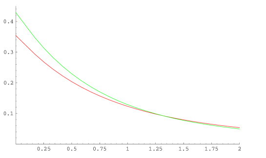
FIG. 1.: The inverse mass $1/\alpha$ is plotted versus $\lambda$ for the two filling factors $\nu=1/2$ (bottom) and $\nu=1/4$ (top)

As a consistency test of the approximation we can verify that the parameter $\kappa$ adjusts its value so that the effect of the interactions is small. Indeed the ratio $\alpha/\alpha^{0}$ where $\alpha^{0}$ is given by (14) has its minimum $.8$ for $\lambda=0$ and increases very fast to $1$. The Coulomb inverse mass ($\lambda=0$) at $\nu=1/2$ is slightly larger than the prediction of Jain and Kamilla [16]: $1/\alpha=.31$. The gaps and the inverse mass decrease very fast with the thickness parameter $\lambda$ which reflects the fact that they are mainly due to the part of the potential of the order of the magnetic length. In order to compare this results with experiments we express the ratio of the effective mass to the bare mass of the electron as [29]:

$${m^{*}\over m_{e}}={\hbar\omega\over V_{c}}$$ (28)

$\hbar\omega=\hbar eB/m_{e}c$ is the cyclotron energy of a bare electron and $V_{c}=e^{2}/\epsilon l$ is the energy scale of the problem ($\epsilon=12.8$ is the dielectric constant for GaAs). It gives ${m^{*}\over m_{e}}=2.63\ 10^{-2}\alpha\sqrt{B}$ ($B$ in tesla). A value of $m^{*}=0.26\sqrt{B}$ in good agreement with the experimental observations [7] is obtained for $\lambda=1.2$ (in units of $l$). This value has been argued by Morf [28] to be a reasonable choice. For this value of $\lambda$ the masses at $\nu=1/4$ and $\nu=1/2$ differ very little, in agreement with Pan et al. [8].

In conclusion we have proposed a simple analytical model to study the FQHE gaps in the vicinity of fillings $\nu=1/2\beta$ with $\beta$ an integer. Its main virtue is to predict microscopically wave functions with no adjustable parameter. Two main feature are predicted. The composite fermion mass depends little on the filling fraction $1/{2\beta}$ as seen in [8] and the gaps collapse with the thickness parameter $\lambda$. The first feature is easy to understand: The filling fraction enters only the definition the Fermi momentum $k_{f}=1/\sqrt{\beta}$ and as long as the CF intraction is weak, the mass depends little on $k_{f}$. The second feature raises questions when we compare this theory to the scaling $m^{*}\propto\sqrt{B}$ seen in [8]. The Thickness parameter $\Lambda=\lambda l$ introduces a new length scale and we see only two ways to explain this scaling. Either $\lambda$ is independent of the density (in other words $\lambda$ scales like $l$) which needs to be explained or the mass depends little on $\lambda$ which contradicts our predictions. We note however that a strong dependence of the gaps in $\Lambda$ may be related to the experimental observation of Shayegan et al [30].

REFERENCES

- [1] J.K.Jain, Phys.Rev.Lett. 63,199 (1989).
- [2] B.A.Halperin, P.A.Lee and N.Read, Phys.Rev.B47,7312 (1993).
- [3] R.L.Willet, Surf.Sci.305, 76 (1994); R.L.Willet et al., Phys.Rev.Lett. 71,3846 (1993).
- [4] W.Kang et al., Phys.Rev.Lett. 71,3850 (1993); V.J. Goldman et al., Phys.Rev.Lett. 72, 2065 (1994); H.J. Smet et al., Phys.Rev.Lett. 77, 2272 (1996).
- [5] L.Saminadayar et al., Phys.Rev.Lett. 79, 2526 (1997); R. de Picciotto et al., Nature 389, 162 (1997).
- [6] E.H.Rezayi and N.Read, Phy.Rev.Lett.72, 900 (1994).
- [7] R.R.Du, H.L.Stormer,D.C.Tsui,N.L.Pfeiffer, and K.W.West, Phys.Rev.Lett. 70, 2944 (1993). P.T.Colerige, Z.W.Wasilewski, P.Zawadzki, A.S. Sacharajda and H.A.Carmona Phys.Rev.B 52 11603 (1995).
- [8] W.Pan,H.L. Stormer,D.C. Tsui,L.N.Pfeiffer,K.W.Baldwin, and K.W.West, cond-mat/9910182.
- [9] F.D.M.Haldane, private communication.
- [10] N.Read,Semicon.Sci.Tech 9, 1859 (1994); Surf.Sci.361,7 (1996).
- [11] V.Pasquier ”Composite Fermions and confinement” (1996) unpublished, to be published in the Morion proceedings (1999).
- [12] R.Shankar and G.Murthy, Phys.Rev.Lett. 79, 4437 (1997).
- [13] Dung-Hai Lee, Phys.Rev.Lett. 80, 4547(1998).
- [14] A.Stern, B.I.Halperin, F. von Oppen, S.Simon, Phys.Rev.B in press and cond mat/9812135.
- [15] V.Pasquier, F.D.M.Haldane Nuclear Physics B 516[FS], 719 (1998).
- [16] J.K.Jain and R.K.Kamilla, Phys. Rev. B 55, R4895 (1997); Int.J.Mod.Phys.B 11,2621 (1997).
- [17] N.Read, Phys.Rev.B58, 16262 (1998).
- [18] L.P.Gor’kov and I.E.Dzyaloshinskii, Sov.Phys.JETP26, 449 (1968).
- [19] I.V.Lerner and Yu.E.Lozovik, Zh Eksp.Theor.Fiz 78, 1167 (1978); [Sov.Phys.JETP51, 588 (1980)].
- [20] C.Kallin and B.I.Halperin, Phys.Rev.B30, 5655 (1984).
- [21] R.Shankar, cond-mat/9903064.
- [22] F.Von Oppen, B.Halperin, S.Simon and A.Stern, cond-mat/9903430.
- [23] F.D.M.Haldane, Phys.Rev.Lett. 51, 605 (1983).
- [24] S.M.Girvin, A.H.Macdonald and P.M.Plazman, Phys.Rev.Lett. 54, 581 (1985).
- [25] G.Murthy , cond-mat/9903187.
- [26] F.C.Zhang and S.Das Sarma, Phys.Rev.B 33, 2903 (1986).
- [27] D.Yoshioka, J.Phys.Soc. Jpn. 55, 885 (1986).
- [28] R.H.Morf, cond mat/9812181
- [29] K.Park and J.K.Jain, Phys.Rev.Lett. 80, 4237 (1997).
- [30] M.Shayegan, J.Jo, Y.W.Suen, M.Santos and V.J.Goldman, Phys.Rev.Lett. 65, 2916 (1990).