Semiclassical theory of the emission properties of wave-chaotic resonant cavities

Abstract

We develop a perturbation theory for the lifetime and emission intensity for isolated resonances in asymmetric resonant cavities. The inverse lifetime $\Gamma$ and the emission intensity $I(\theta)$ in the open system are expressed in terms of matrix elements of operators evaluated with eigenmodes of the closed resonator. These matrix elements are calculated in a semiclassical approximation which allows us to represent $\Gamma$ and $I(\theta)$ as sums over the contributions of rays which escape the resonator by refraction.

The semiclassical theory of wave equations with non-integrable classical (short wavelength) limits has been a topic of great interest over the past decade. Much progress has been made for closed systems based on periodic orbit theory, particularly in the case of fully chaotic systems with no stable periodic orbits or families of regular orbits (KAM tori) [2]. One may for example obtain eigenvalues with an energy resolution inversely proportional to the length of the orbits summed [3]. Much current work addresses the generic case of quantum/wave systems with mixed dynamics in the classical limit, i.e. with stable, unstable and regular regions in phase space [4]. Here we focus on the situation where a system with mixed dynamics is coupled to an infinite asymptotic region and the eigenstates become resonances with complex eigenvalues [5, 6]. A crucial quantity to calculate in this case is the resonance width (imaginary part of the eigenvalue). A basic problem here for semiclassical approaches is that the resonance width may be exponentially smaller than the level spacing, making a direct periodic orbit method very difficult.

Although our approach could be applied to quantum hamiltonians, we will focus here on an important application for such a theory: the formally similar problem of dielectric microcavities. Such resonators are used as high-Q resonators for microlasers and optical spectroscopy [7, 8]. If such resonators are rotationally symmetric the wave equation is separable and analytic solutions for resonance properties are possible; moreover the corresponding ray dynamics (within the resonator) is integrable with conserved angular momentum. When such resonators are deformed from rotational symmetry the ray dynamics is generically mixed and no analytic results were known for resonance properties, except for very small deformations which can then be treated perturbatively [9]. However some time ago [10, 11, 12, 13] it was noted that such asymmetric resonant cavities (ARCs) are equivalent to quantum billiards with refractive escape and a ray-optics model was developed for the lifetime and emission pattern. Although quite successful for low-index resonators where only whispering gallery modes are important, this ray model has several limitations. 1) It only describes quantitatively the whispering gallery modes of such resonators. 2) It neglects all interference effects. 3) It is valid only near a certain adiabatic limit for the phase space flow [12, 13]. However recent experimental results on deformed cylindrical semiconductor microlasers (a high-index, high-gain system) demonstrated high-power and highly directional emission from ”bow-tie” modes which are not well described by this model[14]. Therefore there is both general theoretical and specific experimental motivation for the semiclassical theory of ARCs which we present below.

The key simplification we employ to make the problem tractable is to assume that the eigenstates of the ”closed” system are known and develop a theory which is perturbative in the coupling to the outside but not in the deformation. The resulting analytic formulae are convenient to use in combination with either numerical or semiclassical calculations for the closed problem, and have a simple physical interpretation in terms of refractively escaping rays. For the case of modes associated with stable orbits of the closed system a full analytic semiclassical solution can be found which depends only on $nkR_{0}$ ($k$ is the wavenumber of the radiation, $R_{0}$ is the average radius of the ARC and n is the index of refraction) and properties of the classical orbit (e.g. its period and stability). Finally we note that the numerical solution of such problems becomes intractable due to either instabilities or convergence problems [15] when $kR_{0}$ is of order 100, well below the range of many optical experiments. In this case the semiclassical theory presented here is (to our knowledge) the only available method of solution.

We consider a long cylindrical dielectric resonator of uniform index n with a non–circular cross–section parametrized by the distance $R(\phi)$ between the origin and a point on the the boundary in the $\phi$–direction. We consider the TM polarization (assuming $k_{z}=0$) for which the electric field is perpendicular to the cylinder axis and both the field and its derivative are continuous at the boundary. A quasibound state with complex frequency $\omega=nck$ can be written in the form:

$$E\left({\bf r},t\right)=e^{-ickt}\sum_{m=-\infty}^{\infty}i^{m}A_{m}\left(kr\right)e^{im\phi},$$ (1)

where

$$A_{m} = \left\{\begin{array}[]{ll}\alpha_{m}H_{m}^{+}\left(nkr\right)+\beta_{m}H_{m}^{-}\left(nkr\right)&{\rm if}\ r\leq R(\phi),\\ \gamma_{m}H_{m}^{+}\left(kr\right)&{\rm otherwise}.\end{array}\right.$$ (4)

where $H_{m}^{\pm}$ are Hankel functions. Such resonant solutions can only exist for complex $k$ as there is no incoming wave for $r>R(\phi)$; the imaginary part $\Gamma=-{\rm Im}k$ is the resonance width.

Defining coefficient vectors $\left|\alpha\rangle\right.$, $\left|\beta\rangle\right.$, $\left|\gamma\rangle\right.$ from Eq. (1), the regularity of the wavefunction at $r=0$ requires $\left|\alpha\rangle\right.=\left|\beta\rangle\right.$. Using the continuity conditions to eliminate $\left|\gamma\rangle\right.$ and $\left|\beta\rangle\right.$ the resonance condition can be expressed as the non–hermitian eigenvalue problem

$$\left[{{\cal H}_{0}}\left(k\right)+{V}\left(k\right)\right]\left|\alpha\rangle\right.=0,$$ (5)

where ${\cal H}_{0}$ and $V$ are the hermitian and antihermitian part, respectively, of the matrix ${\cal M}\equiv\left(J^{\prime}J^{\prime}\right)-(1/n)(J^{\prime}{H^{+}}^{\prime})\left(H^{-}H^{+}\right)^{-1}\left(H^{-}J\right)$. Here, ${\cal M}$ is defined in terms of matrices $(Z\bar{Z})$ with matrix elements

$$\left(Z\bar{Z}\right)_{m\ell}=\frac{1}{2\pi}\int d\phi\ Z_{m}\left(k_{0}\right)\bar{Z}_{\ell}\left(k\right)\ e^{i\left(\ell-m\right)\phi},$$ (6)

where $Z_{m}(k)$ and $\bar{Z}_{m}(k)$ stand for either $H^{\pm}_{m}\left(kR\left(\phi\right)\right)$, the Bessel function $J_{m}\left(nkR\left(\phi\right)\right)$, or their derivative, and $k=k_{0}-i\Gamma$.

The perturbation theory is based on the observation that for a narrow resonance $\Gamma\ll\Delta$, (where $\Delta$ is the resonance spacing), the antihermitian term $V$ is a small correction in Eq. (5) which may be expanded in powers of $\Gamma$, to obtain to leading order in $V$:

$$\Gamma = {\langle\alpha^{(0)}\left|V\right|\alpha^{(0)}\rangle\over\langle\alpha^{(0)}\left|\left({\partial{\cal H}_{0}}/{\partial k}\right)\right|\alpha^{(0)}\rangle},$$ (7)

where the matrix elements are taken at the real wave number $\bar{k}_{0}$ defined by the hermitian eigenvalue problem

$${\cal H}_{0}\left(\bar{k}_{0}\right)|\alpha^{(0)}\rangle=0.$$ (8)

The operator ${\cal H}_{0}$ describes a closed resonator with boundary conditions to be specified below. Note, that the denominator in Eq. (7) depends only on the properties of the closed system, and can be regarded as a normalization factor.

Similarly to (7), one can express the far-field emission intensity from the resonance in terms of the eigenstates of ${\cal H}_{0}$,

$$I\left(\theta\right)=|\sum_{m,\ell,\ell^{\prime}}e^{i\ell^{\prime}\theta}\left(H^{-}H^{+}\right)^{-1}_{m\ell}\left(H^{-}J\right)_{\ell\ell^{\prime}}\alpha^{(0)}_{m}|^{2}.$$ (9)

These results represent a general perturbation theory for the problem requiring only small $\Gamma$ and may be of value in their current form. However, far more interesting results can be obtained by taking advantage of the semiclassical limit in which the wavelength of the radiation is assumed much smaller than the average radius of the resonator $nkR_{0}\gg 1$. This condition is satisfied in essentially all optical experiments. In this limit Hankel and Bessel functions may be well-represented by the ”approximation by tangents” [16] and the matrix elements and angular momentum sums in (7), (9) can be evaluated in the stationary phase approximation. In this approximation, the boundary condition corresponding to (8) becomes

$$\left[\nabla_{n}-i\sum_{m}k_{n}\exp\left(i\varphi\right)\left|m\rangle\langle m\right|\right]\left|E\rangle\right.=0,$$ (10)

where $|m\rangle$ is an eigenfunction of angular momentum about the cylinder axis, $\nabla_{n}$ is the normal derivative at the boundary of the resonator and $k_{n}(m,\phi)$ the normal component of the wavevector $\bf k$, and $\varphi\left(k_{n}\right)$ the Fresnel phase change upon reflection from a flat dielectric boundary. When $n\gg 1$, Eq. (10) reduces simply to von Neumann boundary conditions.

We first present the results for $I(\theta)$. Evaluating Eq. (9) in the stationary phase approximation gives three conditions: 1) The matrix $(H^{-}H^{+})^{-1}$ is diagonal. 2) An internal angular momentum $m$ only couples to the angular momentum $l$ which allows the corresponding ray to satisfy Snell’s law (either in transmission or reflection). 3) This ray with angular momentum $\ell_{0}$ must be emitted into angle $\theta$ in the far-field (see Fig. 1a). The last two conditions imply that there exists at most one such ray with angular momentum $\ell_{0}$ for each value of $m,\theta,kR$. If $m$ corresponds to an angle of incidence $\sin\chi\approx m/nkR$ which is totally-internally reflected $(m/kR>1)$ then there is no such ray, and the corresponding component of the field $\alpha_{m}$ does not contribute to emission, hence $I(\theta)$ is only due to refracted rays. At large index the contribution from evanescent escape (tunneling) will be important and is not described by this level of approximation. One finds for the (non–normalized) emission intensity

$$I\left(\theta\right) = \left|\ \Sigma_{m}\exp(im\phi_{\pm})\ e_{m}\left(\theta\right)\alpha_{m}^{(0)}\ \right|^{2},$$ (11)

where $e_{m}\left(\theta\right)=\sum_{\pm}B\left(\phi_{\pm}\right)\exp(i\ell_{0}\left(\theta-\phi_{\pm}-\pi/2\right))$, and

$$B\left(\phi_{\pm}\right)=\frac{H_{\ell_{0}}^{-}\left(kR\right)H_{m}^{\pm}\left(nkR\right)}{H_{\ell_{0}}^{-}\left(kR_{0}\right)H_{\ell_{0}}^{+}\left(kR_{0}\right)}\left[1-2\frac{R^{\prime}}{R}\tan\left(\theta-\phi_{\pm}\right)\right.\ \ \ \ \$$ (12)

$$+\left.\frac{\sec\left(\theta-\phi_{\pm}\right)}{kR}\left[\frac{{R^{\prime\prime}}}{{R^{\prime}}}\left(\ell_{0}-m\right)\pm\frac{\left(R^{\prime}/R\right)^{2}m^{2}}{\sqrt{\left(nkR\right)^{2}-m^{2}}}\right]\right]^{-1/2}.$$ (13)

Here, $\ell_{0}=kR\sin\left(\theta-\phi_{\pm}\right)$ where the $\phi_{\pm}$ are the two distinct points on the boundary where Snell’s law is satisfied for the incident and reflected ray (see Fig. 1a, only incident ray is shown).

Thus Eq. (11) has a simple physical interpretation: $\{\alpha_{m}\}$ describe the relative weight for each angular momentum component in the closed resonator, while the $e_{m}$ are refraction amplitudes describing the probability amplitude for refractive escape from angular momentum $m$ in the direction $\theta$. If the interference terms are neglected in Eq. (11) the result is essentially the ray model of references [10, 11, 12, 13] generalized for an arbitrary initial state, and provides a more rigorous justification for that model. However if one maintains (as we do in Fig. 1) the generality of Eq. (11) including the cross-terms then the interference effects neglected in the ray model are captured.

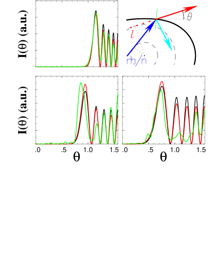
FIG. 1.: Counterclockwise from top right: (a) Schematic of the classical ray emission. (b-d) Far-field emission intensity for a low angular momentum (“bouncing ball”) mode with $nkR\approx 150.$, refractive index $n=1.5$ (b), 2.5 (c), 3.3 (d) and deformation of $\epsilon=0.106$. The black, red and green curves show the exact, perturbative (9) and semiclassical (stationary phase) (11) emission intensities respectively.

In Fig. 1 we show a test of the emission directionality of Eq. (11), comparing to an exact numerically-generated resonance in the resonator with $10\%$ ($\epsilon\approx 0.1$) quadrupolar deformation $R(\phi)=R_{0}(1+\epsilon\cos(2\phi))$, for different values of the refractive index. The exact result (black curve) is very well reproduced by the simple perturbative result of Eq. (9) (red curve) over the whole range of indices of refraction, whereas the semiclassical approximation (Eq. (11), the green curve) works well for the lower indices but not so well for larger index. The origin of this trend is the neglect of the ”non-classical” escape processes mentioned above, which become more important at high index. These tunneling processes are similar to the ”ghost” contributions in periodic orbit theory [17] and can be included by going beyond the real saddles in the stationary-phase approximation as is done in that context. We defer this refinement to future work.

Our theory reduces the calculation of $\Gamma$ and $I(\theta)$ to solving for the eigenstates of the appropriate closed resonator and substituting into Eqs. (7) and (9). In many cases it is possible either to evaluate those eigenstates analytically (e.g. for island or torus states) or to model their statistical properties and hence obtain information about lifetimes and emission patterns in chaotic resonators. As an example, we shall consider the eigenstates localized at the stable islands of the mixed phase space of an ARC. Such eigenstates are of key importance for the recently studied deformed semiconductor microlasers[14], where a factor of $10^{3}$ enhancement of lasing power was attributed to the emission from a mode localized at the stable bow-tie periodic orbit (see inset in Fig. 2a).

We obtain the wave function at the boundary of the resonator using the semiclassical theory developed in Ref. [18]. The quantization on stable islands yields harmonic oscillator wave functions; the corresponding oscillator frequency is determined by the classical dynamics in the vicinity of the periodic orbits. For the ground state resonance, localized at the center of a chain of stable island, we obtain the width

$$\Gamma = \frac{R_{0}}{2\sqrt{\pi}n^{2}}\sum_{\mu}{b\over R_{\mu}\cos^{2}\chi_{\mu}}\int_{-1}^{1}dxe^{-i{b}^{2}\left(x-n\sin\chi_{\mu}\right)^{2}},$$ (14)

where $\chi_{\mu}$ is the periodic orbit incidence angle and $R_{\mu}$ the distance from the bounce point $\mu$. The parameter $b$ measures the ”spread” of the wave function in angular momentum. Choosing as phase space coordinates the arc lenth along the boundary and the transverse momentum $\sin\chi$, one finds $b=(ka_{\mu})/\sqrt{1+a_{\mu}^{4}\left(\eta-f\right)^{2}}$, where $f=s_{\mu}R_{\mu}^{\prime\prime}/R_{\mu}+\left(R_{\mu}^{\prime}/R_{\mu}\right)^{2}\ell^{2}/s_{\mu}$, the angular momentum $\ell$ corresponds to the refracted ray, related to the periodic orbit $\mu$ by $\sin\chi_{\ell}=n\sin\chi_{\mu}$, and $s_{\mu}\equiv\sqrt{\left(kR_{\mu}\right)^{2}-\ell^{2}}$. The parameters $a_{\mu}=\left(4-{\rm Tr}\left[m_{ij}\right]\right)^{1/4}\left(2m_{21}^{\mu}\right)^{-1/2}$ and $\eta_{\mu}=\left(m_{22}^{\mu}-m_{11}^{\mu}\right)/m_{21}^{\mu}$ are defined in term of the monodromy matrix [4] $m_{ij}^{\mu}$. We note that our semiclassical method is justified as long as the area in the phase space “covered” by the eigenstate, is significantly smaller than the size of the islands.

Similar to the calculation of $\Gamma$, we derived a closed semiclassical expression for the emission intensity $I(\theta)$. This calculation will be presented elsewhere [19], one result for the case of the bow-tie resonance is shown in Fig. 2b.

The comparison of the semiclassical emission intensity and width with the exact calculation is presented in Fig. 2. Note, that, as indicated by the Husimi projection of the exact eigenstate (panel (a)), the phase space area of the island is of the order of the effective $\hbar=1/nkR_{0}$. The resulting leakage of amplitude from the island should therefore lead to deviations of the actual intensity from the semiclassical prediction. However, the general structure of the far–field emission pattern (panel (b)) is well reproduced by the semiclassical result.

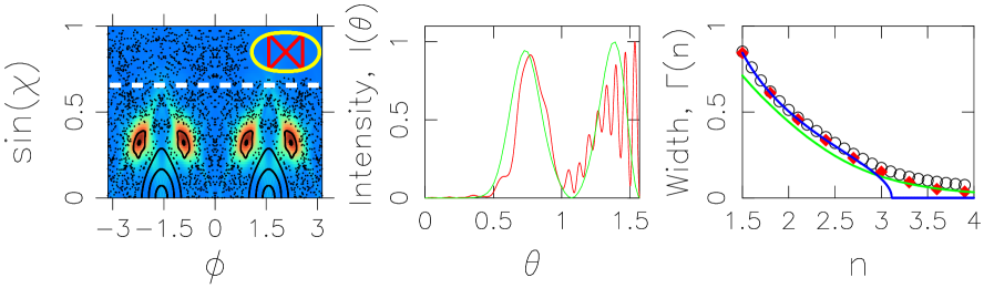
FIG. 2.: The bow-tie resonance, its emission pattern, and its width. (a) Husimi projection (color scale - red denotes high intensity) of bow-tie mode at $n=1.5$, $nkR=102.$, for quadrupolar defomation $\epsilon=0.168$ in $(\phi,\sin\chi)$ coordinates, superimposed on the corresponding Poincaré Surface of Section. The white dashed line indicates the threshold for classical emission, $\sin\chi_{c}=1/n$, above which only tunneling escape occurs. Inset: Schematic of bow-tie periodic orbit. (b) Far-field emission: Exact numerical results (red), and the analytic semiclassical result for this island state (green). The formula leading to the green curve is not given in the text due to space limitations, it will be derived elsewhere [19]. (c) Comparison of the exact width of the bow-tie resonance (circles and diamonds) with the semiclassical (green line) expression (14) and classical (blue line) prediction. Black circles and red diamond correspond to bow-tie resonances close to $nkR_{0}=45.$ and $nkR_{0}=102.$ respectively.

In panel (c) we compare the results for the resonance width. In addition to the exact data points (circles and diamonds) and the semiclassical prediction of Eq. (14) (red curve), we also show the classical result $\Gamma=(2R_{0}/L)\ln r$ (blue curve), based on the Fresnel reflection coefficients $r$, calculated at the incidence angle of the periodic orbit ($L$ here is the total length of the periodic orbit). The simple classical model works very well at index near unity since it is not perturbative in $\Gamma/\Delta$ which is not very small in this case; whereas the semiclassical theory of Eq. (14) is perturbative and shows a small but visible discrepancy in this range. However once the index becomes large enough that a ray on the bow-tie orbit will be totally-internally reflected the classical model gives the unphysical result $\Gamma=0$, whereas our semiclassical model continues to decrease smoothly and in good agreement with the numerical data.

In summary, we have developed a theory of resonance lifetime and emission intensity in nonintegrable dielectric resonators. The theory is in a good agreement with numerical data, has a simple physical interpretation in terms of refractive emission, and gives non-trivial predictions for the lifetimes and emission patterns in asymmetric resonant cavities.

We gratefully acknowledge the support of the NSF grant PHY9612200, the Deutsche Forschungsgemeinschaft, the Swiss National Science Foundation, and the Aspen Center for Physics. We thank Jens Noeckel for useful conversations.

REFERENCES

- [1]
- [2] M.C. Gutzwiller, Chaos in Classical and Quantum Mechanics, (Springer-Verlag, NY, 1990).
- [3] U. Smilansky in Les Houches Session LXI, Eds. E. Akkermans, G. Montambaux, J.-L. Pichard and J. Zinn-Justin (North-Holland, Amsterdam, 1995)
- [4] L. E. Reichl, The Transition To Chaos (Springer-Verlag, New York, 1992).
- [5] P. Gaspard and S.A. Rice, J. Chem. Phys. 90, 2225 (1989); 2242 (1989).
- [6] G. Casati, G. Maspero and D.L. Shepelyansky, Phys. Rev. E 56, R6233 (1997).
- [7] Y. Yamamota and R. E. Slusher, Physics Today 46, 66 (1993).
- [8] M. L. Gorodetsky and V. Ilchenko, J. Opt. Soc. Am. B 16, 147 (1999).
- [9] H.M. Lai et al., Phys. Rev. A, 41, 5187 (1990).
- [10] J. U. Nöckel, A. D. Stone, and R. K. Chang, Opt. Lett. 19, 1693 (1994).
- [11] A. Mekis, J. U. Nöckel, G. Chen, A. D. Stone, and R. K. Chang, Phys. Rev. Lett. 75, 2682 (1995).
- [12] J. U. Nöckel, A. D. Stone, G. Chen, H. Grossman, and R. K. Chang, Opt. Lett. 21, 1609 (1996).
- [13] J. U. Nöckel and A. D. Stone, Nature 385, 47 (1997).
- [14] C. Gmachl, F. Capasso, E. E. Narimanov, J. U. Nöckel, A. D. Stone, J. Faist, D. L. Sivco, and A. Y. Cho, Science 280, 1493 (1998).
- [15] J.P. Barton, J. Appl. Phys. 69, 7973 (1991).
- [16] M. A. Abramowitz and I. Stegun, Handbook of Mathematical Functions, (Dover, NY 1972).
- [17] M. Kus, F. Haake and D. Delande, Phys. Rev. Lett. 71, 2167 (1993).
- [18] E. E. Narimanov, A. D. Stone, and G. S. Boebinger, Phys. Rev. Lett. 80, 4024 (1998); E. E. Narimanov, and A. D. Stone, Physica D 131, 220 (1999).
- [19] G. Hackenbroich, E. E. Narimanov, P. Jacquod, and A. D. Stone, unpublished.