Mean-field theory for scale-free random networks

Abstract

Random networks with complex topology are common in Nature, describing systems as diverse as the world wide web or social and business networks. Recently, it has been demonstrated that most large networks for which topological information is available display scale-free features. Here we study the scaling properties of the recently introduced scale-free model, that can account for the observed power-law distribution of the connectivities. We develop a mean-field method to predict the growth dynamics of the individual vertices, and use this to calculate analytically the connectivity distribution and the scaling exponents. The mean-field method can be used to address the properties of two variants of the scale-free model, that do not display power-law scaling.

PACS:

1 Introduction

Contemporary science has been particularly successful in addressing the physical properties of systems that are composed of many identical elements interacting through mainly local interactions. For example, many successes of materials science and solid state physics are based on the fact that most solids are made of relatively few types of elements that exhibit spatial order by forming a crystal lattice. Furthermore, these elements are coupled by local, nearest neighbor interactions. However, the inability of contemporary science to describe systems composed of non-identical elements that have diverse and nonlocal interactions currently limits advances in many disciplines, ranging from molecular biology to computer science [1]. The difficulty in describing these systems lies partly in their topology: many of them form complex networks, whose vertices are the elements of the system and edges represent the interactions between them. For example, living systems form a huge genetic network, whose vertices are proteins, the edges representing the chemical interactions between them [2]. Similarly, a large network is formed by the nervous system, whose vertices are the nerve cells, connected by axons [3]. But equally complex networks occur in social science, where vertices are individuals, organizations or countries, and the edges characterize the social interaction between them [4], in the business world, where vertices are companies and edges represent diverse business relationships, or describe the world wide web (www), whose vertices are HTML documents connected by links pointing from one page to another [5, 6]. Due to their large size and the complexity of the interactions, the topology of these networks is largely unknown or unexplored.

Traditionally, networks of complex topology have been described using the random graph theory of Erdős and Rényi (ER) [7]. However, while it has been much investigated in combinatorial graph theory, in the absence of data on large networks the predictions of the ER theory were rarely tested in the real world. This is changing very fast lately: driven by the computerization of data acquisition, topological information on various real world networks is increasingly available. Due to the importance of understanding the topology of some of these systems, it is likely that in the near future we will witness important advances in this direction. Furthermore, it is also possible that seemingly random networks in Nature have rather complex internal structure, that cover generic features, common to many systems. Uncovering the universal properties characterizing the formation and the topology of complex networks could bring about the much coveted revolution beyond reductionism [1].

A major step in the direction of understanding the generic features of network development was the recent discovery of a surprising degree of self-organization characterizing the large scale properties of complex networks. Exploring several large databases describing the topology of large networks, that span as diverse fields as the www or the citation patterns in science, recently Barabási and Albert (BA) have demonstrated[8] that independently of the nature of the system and the identity of its constituents, the probability $P(k)$ that a vertex in the network is connected to $k$ other vertices decays as a power-law, following $P(k)\sim k^{-\gamma}$. The generic feature of this observation was supported by four real world examples. In the collaboration graph of movie actors, each actor is represented by a vertex, two actors being connected if they were casted in the same movie. The probability that an actor has $k$ links was found to follow a power-law for large $k$, i.e. $P(k)\sim k^{-\gamma_{actor}}$, where $\gamma_{actor}=2.3\pm 0.1.$ A rather complex network with over $300$ million vertices [9] is the www, where a vertex is a document and the edges are the links pointing from one document to another. The topology of this graph determines the web’s connectivity and, consequently, our effectiveness in locating information on the www [5]. Information about $P(k)$ can be obtained using robots [6], indicating that the probability that $k$ documents point to a certain webpage follows a power-law, with $\gamma_{www}^{in}=2.1$ [10], and the probability that a certain web document contains $k$ outgoing links follows a similar distribution, with $\gamma_{www}^{out}=2.45$. A network whose topology reflects the historical patterns of urban and industrial development is the electrical powergrid of western US, the vertices representing generators, transformers and substations, the edges corresponding to the high voltage transmission lines between them [13]. The connectivity distribution is again best approximated with a power-law with an exponent $\gamma_{power}\simeq 4$. Finally, a rather large, complex network is formed by the citation patterns of the scientific publications, the vertices standing for papers, the edges representing links to the articles cited in a paper. Recently Redner [14] has shown that the probability that a paper is cited $k$ times (representing the connectivity of a paper within the network) follows a power-law with exponent $\gamma_{cite}=3$. These results offered the first evidence that large networks self-organize into a scale-free state, a feature unexpected by all existing random network models. To understand the origin of this scale invariance, BA have shown that existing network models fail to incorporate two key features of real networks: First, networks continuously grow by the addition of new vertices, and second, new vertices connect preferentially to highly connected vertices. Using a model incorporating these ingredients, they demonstrated that the combination of growth and preferential attachment is ultimately responsible for the scale-free distribution and power-law scaling observed in real networks.

The goal of the present paper is to investigate the properties of the scale-free model introduced by BA [8], aiming to identify its scaling properties and compare them with other network models intended to describe the large scale properties of random networks. We present a mean field theory that allows us to predict the dynamics of individual vertices in the system, and to calculate analytically the connectivity distribution. We apply the same method to uncover the scaling properties of two versions of the BA model, that are missing one of the ingredients needed to reproduce the power-law scaling. Finally, we discuss various extensions of the BA model, that could be useful in addressing the properties of real networks.

2 Earlier network models

2.1 The Erdős-Rényi model

Probably the oldest and most investigated random network model has been introduced by Erdős and Rényi (ER) [7], who were the first to study the statistical aspects of random graphs by probabilistic methods. In the model we start with $N$ vertices and no bonds (see Fig. 1a). With probability $p_{\mathrm{ER}}$, we connect each pair of vertices with a line (bond or edge), generating a random network. The greatest discovery of ER was that many properties of these graphs appear quite suddenly, at a threshold value of $p_{\mathrm{ER}}(N)$. A property of great importance for the topology of the graph is the appearance of trees and cycles. A tree of order $k$ is a connected graph with $k$ vertices and $k-1$ edges, while a cycle of order $k$ is a cyclic sequence of $k$ edges such that every two consecutive edges and only these have a common vertex. ER have demonstrated that if $p_{\mathrm{ER}}\sim c/N$ with $c<1$, then almost all vertices belong to isolated trees, but there is an abrupt change at $p_{\mathrm{ER}}\sim 1/N$, (i.e. $c=1$), when cycles of all orders appear. In the physical literature the ER model is often referred to as infinite dimensional percolation, that is known to belong to the universality class of mean field percolation [15]. In this context $p_{c}\sim 1/N$ is the percolation threshold of the system. For $p<p_{c}$ the system is broken into many small clusters, while at $p_{c}$ a large cluster forms, that in the asymptotic limit contains all vertices.

To compare the ER model with other network models, we need to focus on the connectivity distribution. As Erdős and Rényi have shown in their seminal work, the probability that a vertex has $k$ edges follows the Poisson distribution

$$P(k)=e^{-\lambda}{\lambda}^{k}/k!,$$ (1)

where

$$\lambda=\left(\begin{array}[]{c}N-1\\ k\end{array}\right)p_{\mathrm{ER}}^{k}(1-p_{\mathrm{ER}})^{N-1-k},$$ (2)

its expectation value being $(N-1)p_{\mathrm{ER}}$. For sake of comparison, in Fig. 2a we show $P(k)$ for different values of $p_{\mathrm{ER}}$.

Figure 1: Schematic illustration of the Erdős-Rényi (ER) and Watts-Strogatz (WS) models. (a) A random network described by the ER model has N vertices connected with probability $p_{\mathrm{ER}}$, the total number of edges in the system being $n=p_{\mathrm{ER}}N(N-1)/2$. The example presents a network of $N=10$ vertices for $p_{\mathrm{ER}}=0$ and $p_{\mathrm{ER}}=0.2$. At $p_{\mathrm{ER}}=0$ there are no edges in the system. We select each pair of vertices and connect them with probability $p_{\mathrm{ER}}=0.2$. The figure shows the result of this process, the network having $n=9$ edges. For $p_{\mathrm{ER}}=1$ the model leads to a fully connected network. (b) The WS model starts with a regular one dimensional lattice with edges between the nearest and next-nearest neighbors, thus the average connectivity is $\langle k\rangle=4$. Then a fraction $p_{\mathrm{WS}}$ of the edges is rewired randomly (their endpoint is changed to a randomly selected vertex). The example presents a network of $N=10$ vertices. For $p_{\mathrm{WS}}=0$ the system is a regular lattice with $2N=20$ edges. For $p_{\mathrm{WS}}=0.3$, $2p_{\mathrm{WS}}N=6$ edges have been rewired to randomly selected vertices. Note that for $p_{\mathrm{WS}}=1$ we obtain a random network, equivalent to that obtained for the ER model with $p_{\mathrm{ER}}=\langle k\rangle/N=0.4$.

2.2 The small-world model

Aiming to describe the transition from a locally ordered system to a random network, recently Watts and Strogatz (WS) have introduced a new model [13], that is often referred to as small-world network. The topological properties of the network generated by this model have been the subject of much attention lately [16, 17, 18, 19, 20, 21, 22, 23, 24, 25, 26, 27, 28]. The WS model begins with a one-dimensional lattice of $N$ vertices with bonds between the nearest and next-nearest neighbors (in general, the algoritm can include neighbors up to an order $n$, such that the coordination number of a vertex is $z=2n$) and periodic boundary conditions (see Fig. 1b). Then each bond is rewired with probability $p_{\mathrm{WS}}$, where rewiring in this context means shifting one end of the bond to a new vertex chosen at random from the whole system, with the constraint that no two vertices can have more than one bond, and no vertex can have a bond with itself. For $p_{\mathrm{WS}}=0$ the lattice is highly clustered, and the average distance between two vertices $\langle l\rangle$ grows linearly with $N$, while for $p_{\mathrm{WS}}=1$ the system becomes a random graph, poorly clustered and $\langle l\rangle$ grows logarithmically with $N$. WS found that in the interval $0<p_{\mathrm{WS}}<0.01$ the model exhibits small-world properties[29], ($\langle l\rangle\simeq\langle l\rangle_{random}$), while it remains highly clustered.

The connectivity distribution of the WS model depends strongly on $p_{\mathrm{WS}}$: for $p_{\mathrm{WS}}=0$ we have $P(k)=\delta(k-z)$, where $z$ is the coordination number of the lattice, while for finite $p_{\mathrm{WS}}$, $P(k)$ is still peaked around $z$, but it gets broader. Ultimately, as $p_{\mathrm{WS}}\rightarrow 1$, the distribution $P(k)$ approaches the connectivity distribution of a random graph, i.e. the distribution converges to that obtained for the ER model with $p_{\mathrm{ER}}=z/N$ (see Fig. 2b).

Figure 2: Connectivity distributions for the ER and WS models. (a) $P(k)$ in the ER model for $N=10,000$ and for $p_{\mathrm{ER}}=0.0006$ (circles), $p_{\mathrm{ER}}=0.001$ (squares) and $p_{\mathrm{ER}}=0.0015$ (diamonds). (b) $P(k)$ in the WS model for $N=10,000$, $\langle k\rangle=6$ and three rewiring probabilities $p_{\mathrm{WS}}=0$ (circle, corresponding to the delta-function $\delta(k-6)$), $p_{\mathrm{WS}}=0.1$ (squares) and $p_{\mathrm{WS}}=0.3$ (diamonds).

3 The scale-free model

A common feature of the models discussed in the previous section is that they both predict that the probability distribution of the vertex connectivity, $P(k)$, has an exponential cutoff, and has a characteristic size $\left<k\right>$, that depends on $p$. In contrast, as we mentioned in the Introduction, many systems in nature have the common property that $P(k)$ is free of scale, following a power-law distribution over many orders of magnitude. To understand the origin of this discrepancy, BA have argued that there are two generic aspects of real networks that are not incorporated in these models [8]. First, both models assume that we start with a fixed number ($N$) of vertices, that are then randomly connected (ER model), or reconnected (SW model), without modifying $N$. In contrast, most real world networks are open, i.e. they form by the continuous addition of new vertices to the system, thus the number of vertices, $N$, increases throughout the lifetime of the network. For example, the actor network grows by the addition of new actors to the system, the www grows exponentially in time by the addition of new web pages, the research literature constantly grows by the publication of new papers. Consequently, a common feature of these systems is that the network continuously expands by the addition of new vertices that are connected to the vertices already present in the system.

Second, the random network models assume that the probability that two vertices are connected is random and uniform. In contrast, most real networks exhibit preferential connectivity. For example, a new actor is casted most likely in a supporting role, with more established, well known actors. Similarly, a newly created webpage will more likely include links to well known, popular documents with already high connectivity, or a new manuscript is more likely to cite a well known and thus much cited paper than its less cited and consequently less known peer. These examples indicate that the probability with which a new vertex connects to the existing vertices is not uniform, but there is a higher probability to be linked to a vertex that already has a large number of connections. The scale-free model introduced by BA, incorporating only these two ingredients, naturally leads to the observed scale invariant distribution. The model is defined in two steps (see Fig. 3):

(1) Growth: Starting with a small number ($m_{0}$) of vertices, at every timestep we add a new vertex with $m$($\leq m_{0}$) edges (that will be connected to the vertices already present in the system).

(2) Preferential attachment: When choosing the vertices to which the new vertex connects, we assume that the probability $\Pi$ that a new vertex will be connected to vertex $i$ depends on the connectivity $k_{i}$ of that vertex, such that

$$\Pi(k_{i})=k_{i}/\sum_{j}k_{j}.$$ (3)

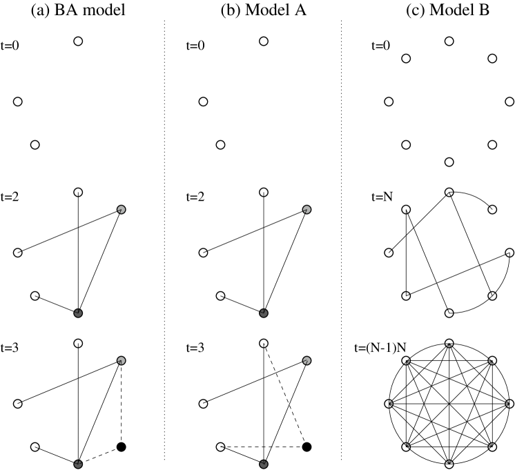
Figure 3: Illustration of the BA model and its variants. (a) BA model for $m_{0}=3$ and $m=2$. At $t=0$ the system consists of $m_{0}=3$ isolated vertices. At every timestep a new vertex is added, which is connected to $m=2$ vertices, preferentially to the vertices with high connectivity, determined by the rule (3). Thus at $t=2$ there are $m_{0}+t=5$ vertices and $mt=4$ edges. At $t=3$ the sixth vertex is added, the two new edges being drawn with dashed lines. Due to preferential attachment the new vertex was linked to vertices with already high connectivity. (b) Model A with $m_{0}=3$ and $m=2$. At $t=0$ there are $m_{0}=3$ vertices and no edges. At every timestep a new vertex is added to the system, which is connected randomly to $m=2$ vertices already present. As in (a), at $t=2$ there are five vertices and four edges. At $t=3$ the sixth vertex is added to the system. The two new edges are drawn with dashed lines. Since preferential attachment is absent, the new vertex connects with equal probability to any vertex in the system. (c) Model B with $N=8$ vertices. In this model the number of vertices is fixed. At $t=0$ there are no edges. At every step a new edge is introduced, one end being added to a randomly selected vertex, the other end folowing preferential attachment (3). At $t=N$ there are eight edges in the considered example, while at $t=N(N-1)/2$ the system is fully connected.

After $t$ timesteps the model leads to a random network with $N=t+m_{0}$ vertices and $mt$ edges. As Fig. 4a shows, this network evolves into a scale-invariant state, the probability that a vertex has $k$ edges following a power-law with an exponent $\gamma_{model}=2.9\pm 0.1$. The scaling exponent is independent of $m$, the only parameter in the model. Since the power-law observed for real networks describes systems of rather different sizes at different stages of their development, one expects that a correct model should provide a distribution whose main features are independent of time. Indeed, as Fig. 4b demonstrates, $P(k)$ is independent of time (and, subsequently, independent of the system size $N=m_{0}+t$), indicating that despite its continuous growth, the system organizes itself into a scale-free stationary state.

Figure 4: (a) Connectivity distribution of the BA model, with $N=m_{0}+t=300,000$ and $m_{0}=m=1$ (circles), $m_{0}=m=3$ (squares), $m_{0}=m=5$ (diamonds) and $m_{0}=m=7$ (triangles). The slope of the dashed line is $\gamma=2.9$. The inset shows the rescaled distribution (see text) $P(k)/2m^{2}$ for the same values of $m$, the slope of the dashed line being $\gamma=3$. (b) $P(k)$ for $m_{0}=m=5$ and system sizes $N=100,000$ (circles), $N=150,000$ (squares) and $N=200,000$ (diamonds). The inset shows the time-evolution for the connectivity of two vertices, added to the system at $t_{1}=5$ and $t_{2}=95$. Here $m_{0}=m=5$, and the dashed line has slope $0.5$, as predicted by Eq. (6).

We next describe a method to calculate analytically the probability $P(k)$, allowing us to determine exactly the scaling exponent $\gamma$. The combination of growth and preferential attachment leads to an interesting dynamics of the individual vertex connectivities. The vertices that have the most connections are those that have been added at the early stages of the network development, since vertices grow proportionally to their connectedness relative to the rest of the vertices. Thus some of the oldest vertices have a very long time to acquire links, being responsible for the high-$k$ part of $P(k)$. The time dependence of the connectivity of a given vertex can be calculated analytically using a mean-field approach. We assume that $k$ is continuous, and thus the probability $\Pi(k_{i})=k_{i}/\sum_{j}k_{j}$ can be interpreted as a continuous rate of change of $k_{i}$. Consequently, we can write for a vertex $i$

$$\frac{\partial k_{i}}{\partial t}=A\Pi(k_{i})=A\frac{k_{i}}{\sum_{j=1}^{m_{0}+t-1}k_{j}}.$$ (4)

Taking into account that $\sum_{j}k_{j}=2mt$ and the change in connectivities at a time step is $\Delta(k)=m$, we obtain that $A=m$, leading to

$$\frac{\partial k_{i}}{\partial t}=\frac{k_{i}}{2t}.$$ (5)

The solution of this equation, with the initial condition that vertex $i$ was added to the system at time $t_{i}$ with connectivity $k_{i}(t_{i})=m$, is

$$k_{i}(t)=m\left(\frac{t}{t_{i}}\right)^{0.5}.$$ (6)

As the inset of Fig. 4b shows, the numerical results are in good agreement with this prediction. Thus older (smaller $t_{i}$) vertices increase their connectivity at the expense of the younger (larger $t_{i}$) vertices, leading with time to some vertices that are highly connected, a “rich-gets-richer” phenomenon that can be easily detected in real networks. Furthermore, this property can be used to calculate $\gamma$ analytically. Using (6), the probability that a vertex has a connectivity $k_{i}(t)$ smaller than $k$, $P(k_{i}(t)<k)$, can be written as

$$P(k_{i}(t)<k)=P(t_{i}>{{m^{2}t}\over{k^{2}}}).$$ (7)

Assuming that we add the vertices at equal time intervals to the system, the probability density of $t_{i}$ is

$$P_{i}(t_{i})=\frac{1}{m_{0}+t}.$$ (8)

Substituting this into Eq. (4) we obtain that

$$P(t_{i}>{{m^{2}t}\over{k^{2}}})=1-P(t_{i}\leq{{m^{2}t}\over{k^{2}}})=1-{{m^{2}t}\over{k^{2}(t+m_{0})}}.$$ (9)

The probability density for $P(k)$ can be obtained using

$$P(k)=\frac{\partial P(k_{i}(t)<k)}{\partial k}=\frac{2m^{2}t}{m_{0}+t}\,\frac{1}{k^{3}},$$ (10)

predicting

$$\gamma=3,$$ (11)

independent of $m$. Furthermore, Eq. (10) also predicts that the coefficient $A$ of the power-law distribution, $P(k)\sim Ak^{-\gamma}$, is proportional to the square of the average connectivity of the network, i.e., $A\sim m^{2}$. In the inset of Fig. 4a we show $P(k)/2m^{2}$ vs. $k$. The curves obtained for different $m$ collapse into a single one, supporting the analytical result (10).

4 Limiting cases of the scale-free model

4.1 Model A

The development of the power-law scaling in the scale-free model indicates that growth and preferential attachment play an important role in network development. To verify that both ingredients are necessary, we investigated two variants of the BA model. The first variant, that we refer to as model A, keeps the growing character of the network, but preferential attachment is eliminated. The model is defined as follows (see Fig. 3b):

(1) Growth : Starting with a small number of vertices ($m_{0}$), at every time step we add a new vertex with $m(\leq m_{0})$ edges.

(2) Uniform attachment : We assume that the new vertex connects with equal probability to the vertices already present in the system, i.e. $\Pi(k_{i})=1/(m_{0}+t-1)$, independent of $k_{i}$.

Fig. 5a shows the probability $P(k)$ obtained for different values of $m$, indicating that in contrast with the scale-free model, $P(k)$ has an exponential form

$$P(k)=B\exp(-\beta k)$$ (12)

Figure 5: (a) The connectivity distribution for model A for $m_{0}=m=1$ (circles), $m_{0}=m=3$ (squares), $m_{0}=m=5$ (diamonds) and $m_{0}=m=7$ (triangles). The system size is $N=800,000$. The inset presents the scaling of the coefficients $B$ and $\beta$ (see Eq. (12)) with $m$, the dashed line following the prediction (18). (b) Time evolution for the connectivity of two vertices added to the system at $t_{1}=7$ and $t_{2}=97$. Here $m_{0}=m=3$. The dashed line follows $k_{i}(t)=m\ln(m_{0}+t-1)$ as predicted by (14).

We can use the mean field arguments developed in the previous section to calculate analytically the expression for $P(k)$. The rate of change of the connectivity of vertex $i$ in this case is given by

$$\frac{\partial k_{i}}{\partial t}=A\Pi(k_{i})=\frac{A}{m_{0}+t-1}.$$ (13)

At one timestep $\Delta(k)=m$, implying that $A=m$. Solving the equation for $k_{i}$, and taking into account that $k_{i}(t_{i})=m$, we obtain

$$k_{i}=m\left(\ln(m_{0}+t-1)-\ln(m_{0}+t_{i}-1)+1\right),$$ (14)

a logarithmic increase with time, verified by the numerical simulations (see Fig. 5b).

The probability that vertex $i$ has connectivity $k_{i}(t)$ smaller than $k$ is

$$P(k_{i}(t)<k)=P\left(t_{i}>(m_{0}+t-1)\exp(1-\frac{k}{m})-m_{0}+1\right).$$ (15)

Assuming that we add the vertices uniformly to the system, we obtain that

$$P\left(t_{i}>(m_{0}+t-1)\exp(1-\frac{k}{m})-m_{0}+1\right)$$

$$=1-\frac{(m_{0}+t-1)\exp(1-\frac{k}{m})-m_{0}+1}{m_{0}+t}.$$ (16)

Using Eq. (10) and assuming long times, we obtain

$$P(k)=\frac{e}{m}\exp(-\frac{k}{m}),$$ (17)

indicating that in (12) the coefficients are

$$B=\frac{e}{m},~{}~{}\beta=\frac{1}{m}.$$ (18)

Consequently, the vertices in the model have the characteristic connectivity

$$k^{*}={1\over\beta}=m,$$ (19)

which coincides with half of the average connectivities of the vertices in the system, since $\left<k\right>=2m$. As the inset of Fig. 5a demonstrates the numerical results approach asymptotically the theoretical predictions. The exponential character of the distribution for this model indicates that the absence of preferential attachment eliminates the scale-free feature of the BA model.

4.2 Model B

This model tests the hypothesis that the growing character of the model is essential to sustain the scale-free state observed in the real systems. Model B is defined as follows (see Fig. 3c):

We start with $N$ vertices and no edges. At each time step we randomly select a vertex and connect it with probability $\Pi(k_{i})=k_{i}/\sum_{j}k_{j}$ to vertex $i$ in the system.

Consequently, in comparison with the BA model, this variant eliminates the growth process, the numbers of vertices staying constant during the network evolution. While at early times the model exhibits power-law scaling (see Fig. 6, $P(k)$ is not stationary: Since $N$ is constant, and the number of edges increases with time, after $T\simeq N^{2}$ timesteps the system reaches a state in which all vertices are connected.

The time-evolution of the individual connectivities can be calculated analytically using the mean field approximation developed for the previous models. The rate of change of the connectivity of vertex $i$ has two contributions: the first describes the probability that the vertex is chosen randomly as the origin of the link, $\Pi_{random}(k_{i})=1/N$ and the second is proportional to $\Pi(k_{i})=k_{i}/\sum_{j}k_{j}$, describing the probability that an edge originating from a randomly selected vertex is linked to vertex $i$:

$$\frac{\partial k_{i}}{\partial t}=A\frac{k_{i}}{\sum_{j=1}^{N}k_{j}}+\frac{1}{N}.$$ (20)

Taking into account that $\sum_{j}k_{j}=2t$ and that the change in connectivities during one timestep is $\Delta(k)=2$, and excluding from the summation edges originating and terminating in the same vertex, we obtain $A=N/(N-1)$, leading to

$$\frac{\partial k_{i}}{\partial t}=\frac{N}{N-1}\,\frac{k_{i}}{2t}+\frac{1}{N}.$$ (21)

The solution of this equation has the form

$$k_{i}(t)=\frac{2(N-1)}{N(N-2)}t+Ct^{\frac{N}{2(N-1)}}.$$ (22)

Since $N>>1$, we can approximate $k_{i}$ with

$$k_{i}(t)=\frac{2}{N}t+Ct^{1/2}$$ (23)

Since the number of vertices is constant, we do not have “introduction times” $t_{i}$ for the vertices. There exists, however, a time time analogous to $t_{i}$: the time when vertex $i$ was selected for the first time as the origin of an edge, and consequently its connectivity changed from $0$ to $1$. Equation (22) is valid only for $t>t_{i}$, and all vertices will follow this dynamics only after $t\geq N$. The constant $C$ can be determined from the condition that $\sum_{j}k_{j}=2t$, and has the value

$$C=0,$$ (24)

thus

$$k_{i}(t)\simeq\frac{2}{N}t.$$ (25)

The numerical results shown in Fig. 6b agree well with this prediction, indicating that after a transient time of duration $t\simeq N$ the connectivity increases linearly with time.

Figure 6: (a) The connectivity distribution for model B for $N=10,000$ and $t=N$ (circles), $t=5N$ (squares), and $t=40N$ (diamonds) and $t=40N$. (b) Time dependence of the connectivities of two vertices. The system size is $N=10,000$. The inset shows the connectivities rescaled by $N/2t$, supporting the theoretical prediction $k_{i}(t)N/2t\rightarrow 1$.

Since the mean-field approximation used above predicts that after a transient period the connectivities of all vertices should have the same value given by Eq. (25), we expect that the connectivity distribution becomes a Gaussian around its mean value. Indeed, Fig. 6a illustrates that as time increases, the shape of $P(k)$ changes from the initial power-law to a Gaussian.

The failure of models A and B in leading to a scale-free distribution indicates that both ingredients, namely growth and preferential attachment, are needed to reproduce the stationary power-law distribution observed in real networks.

5 Discussion and conclusions

In the following we discuss some of the immediate extensions of the present work.

(i) A major assumption in the model was the use of a linear relationship between $\Pi(k_{i})$ and $k_{i}$, given by (3). However, at this point there is nothing to guarantee us that $\Pi(k)$ is linear, i.e. in general we could assume that $\Pi(k)\sim k^{\alpha}$, where $\alpha\neq 1$. The precise form of $\Pi(k)$ could be determined numerically by comparing the topology of real networks at not too distant times. In the absence of such data, the linear relationship seems to be the most efficient way to go. In principle, if nonlinearities are present (i.e. $\alpha\neq 1$), that could affect the nature of the power-law scaling. This problem will be addressed in future work [30].

(ii) An another quantity that could be tested explicitelly is the time evolution of connectivities in real networks. For the scale-free model we obtained that the connectivity increases as a power of time (See Eq. (6)). For model A we found logarithmic time dependence (Eq. (14)), while for model B linear (Eq. (25)). Furthermore, if we introduce $p_{\mathrm{ER}}=at$ in the ER model, one can easily show that $\langle k\rangle_{\mathrm{ER}}(t)\sim t$. If time resolved data on network connectivity becomes available, these predictions could be explicitelly tested for real networks, allowing us to distinguish between the different growth mechanisms.

(iii) In the model we assumed that new links appear only when new vertices are added to the system. In many real systems, including the movie actor networks or the www, links are added continuously. Our model can be easily extended to incorporate the addition of new edges. Naturally, if we add too many edges, the system becomes fully connected. However, in most systems the addition of new vertices (and the growth of the system) competes with the addition of new internal links. As long as the growth rate is large enough, we believe that the system will remain in the universality class of the BA model, and will continue to display scale-free features.

(iv) Naturally, in some systems we might witness the reconnection or rewiring of the existing links. Thus some links, that were added when a new vertex was added to the system, will break and reconnect with other vertices, probably still obeying preferential attachment. If reattachment dominates over growth (i.e. addition of new links by new vertices), the system will undergo a process similar to ripening: the very connected sites will acquire all links. This will destroy the power-law scaling in the system. However, similarly to case (iii) above, as long as the growth process dominates the dynamics of the system, we expect that the scale-free state will prevail.

(v) The above discussion indicates that there are a number of “end-states” or absorbing states for random networks, that include the scale-free state, when power-law scaling prevails at all times, the fully connected state, which will be the absorbing state of the ER model for large $p$, and the ripened state, which will characterize the system described in point (iv). Note that the end state of the WS model, obtained for $p_{\mathrm{WS}}=1$, is the ER model for $p_{\mathrm{ER}}=z/N$. The precise nature of the transition between these states is still an open question, and will be the subject of future studies [30].

(vi) Finally, the concept of universality classes has not been properly explored yet in the context of random network models. For this we have to define scaling exponents that can be measured for all random networks, whether they are generated by a model or a natural process. The clustering of these exponents for different systems might indicate that there are a few generic universality classes characterizing complex networks. Such studies have the potential to lead to a better understanding of the nature and growth of random networks in general.

Growth and preferential attachment are mechanisms common to a number of complex systems, including business networks [31], social networks (describing individuals or organizations), transportation networks [32], etc. Consequently, we expect that the scale-invariant state, observed in all systems for which detailed data has been available to us, is a generic property of many complex networks, its applicability reaching far beyond the quoted examples. A better description of these systems would help in understanding other complex systems as well, for which so far less topological information is available, including such important examples as genetic or signaling networks in biological systems. Similar mechanisms could explain the origin of the social and economic disparities governing competitive systems, since the scale-free inhomogeneities are the inevitable consequence of self-organization due to the local decisions made by the individual vertices, based on information that is biased towards the more visible (richer) vertices, irrespective of the nature and the origin of this visibility.

References

- [1] R. Gallagher, T. Appenzeller, Science 284 (1999) 79; R. F. Service, Science 284 (1999) 80.
- [2] G. Weng, U. S. Bhalla, R. Iyengar, Science 284 (1999) 92.
- [3] C. Koch, G. Laurent, Science 284 (1999) 96.
- [4] S. Wasserman, K. Faust, Social Network Analysis (Cambridge University Press, Cambridge, 1994).
- [5] Members of the Clever project, Sci. Am. 280 (June 1999) 54.
- [6] R. Albert, H. Jeong, A.-L. Barabási, cond-mat/9907038.
- [7] P. Erdős, A. Rényi, Publ. Math. Inst. Hung. Acad. Sci. 5 (1960) 17; B. Bollobás, Random Graphs (Academic Press, London, 1985).
- [8] A.-L. Barabási and R. Albert (preprint, available from ralbert@nd.edu).
- [9] S. Lawrence, C. L. Giles, Science 280 (1998) 98.
- [10] Note that in addition to the distribution of incoming links, the www displays a number of other scale-free features, characterizing the organization of the webpages within a domain [11], the distribution of searches [12], or the number of links per webpage [6].
- [11] B. A. Huberman, L. A. Adamic, cond-mat/9901071.
- [12] B. A. Huberman, P. L. T. Pirolli, J. E. Pitkow, R. J. Lukose, Science 280 (1998) 95.
- [13] D. J. Watts, S. H. Strogatz, Nature 393 (1998) 440.
- [14] S. Redner, European Physical Journal B 4 (1998) 131.
- [15] D. Stauffer and A. Aharony, Percolation Theory (Taylor Francis, London, 1992).
- [16] M. Barthélémy, L. A. N. Amaral, Phys. Rev. Lett. 82 (1999) 15.
- [17] J. Collins, C. Chow, Nature 393 (1998) 6684.
- [18] G. Lubkin, Phys. Today 51 (1998) 17.
- [19] H. Herzel, Fractals 6 (1998) 301.
- [20] A. Barrat, cond-mat/9903323.
- [21] R. Monasson, cond-mat/9903347.
- [22] M. E. J. Newman, D. J. Watts, cond-mat/9903357; ibid, cond-mat/9904419.
- [23] A. Barrat, M. Weigt, cond-mat/9903411.
- [24] M. A. Menezes, C. Moukarzel, T. J. P. Penna, cond-mat/9903426.
- [25] R. Kasturirangan, cond-mat/9904055.
- [26] R. V. Kulkarni, E. Almaas, D. Stroud, cond-mat/9905066.
- [27] C. F. Moukarzel, M. A. Menezes, cond-mat/9905131.
- [28] C. F. Moukarzel, cond-mat/9905322.
- [29] S. Milgram, Psychol. Today 2 (1967) 60; M. Kochen (ed.) The Small World (Ablex, Norwood, NJ, 1989).
- [30] R. Albert, H. Jeong, A.-L. Barabási (to be published).
- [31] W. B. Arthur, Science 284 (1999) 107.
- [32] J. R. Banavar, A. Maritan, A. Rinaldo, Nature 399 (1999) 130.