Distribution of fractal dimensions at the Anderson transition

Abstract

We investigated numerically the distribution of participation numbers in the 3d Anderson tight-binding model at the localization-delocalization threshold. These numbers in one disordered system experience strong level-to-level fluctuations in a wide energy range. The fluctuations grow substantially with increasing size of the system. We argue that the fluctuations of the correlation dimension, $D_{2}$ of the wave functions are the main reason for this. The distribution of these correlation dimensions at the transition is calculated. In the thermodynamic limit ($L\to\infty$) it does not depend on the system size $L$. An interesting feature of this limiting distribution is that it vanishes exactly at $D_{\rm 2max}=1.83$, the highest possible value of the correlation dimension at the Anderson threshold in this model.

The localization-delocalization Anderson transition has posed for a long time a fascinating problem. In systems with short range interaction, purely diagonal disorder and unbroken time-reversal symmetry, without spin-orbit interaction, it occurs for dimensions $d>2$ [1]. In the thermodynamic limit (i.e. infinite system size) the transition point separates the systems where all wave functions are localized from the systems where some part of them is extended. Exactly at the transition one finds in the center of the band extended wave functions. Due to the proximity of the unavoidable localization at one side of the transition they have a self-similar fractal (actually multifractal) structure. This is a direct consequence of quantum critical fluctuations at the transition point.

This multifractality of the wave functions at the localization threshold is one of the most important features discovered [2, 3] since the pioneering work of Anderson [4]. This fruitful idea has became widely recognized (see e.g. Refs. [5, 6, 7]) and has considerably helped our understanding of different phenomena in mesoscopic systems related to electron localization. For instance the well known log-normal distribution of the conductance in disordered metals [8] can be taken as a finger-print of multifractal wave functions which survive in the weakly disordered state (so-called pre-localized states [7]).

Usually the multifractal (as well as fractal) structure of a wave function manifests itself in the size dependence of the participation number (PN)

$${\cal N}=\left(\int\left|\psi({\bf r})\right|^{4}d{\bf r}\right)^{-1}\propto L^{D_{2}},$$ (1)

where $L$ is the system size and $D_{2}<d$ is the correlation dimension of the wave function $\psi({\bf r})$. For a localized state $D_{2}=0$ and ${\cal N}$ do not depend on $L$. On the other hand $D_{2}=d$ for a delocalized wave function which extends uniformly over the sample. The inequality $0<D_{2}<d$ means that a multifractal wave function is delocalized but, in the thermodynamic limit, nevertheless occupies only an infinitesimal fraction of the sample.

Due to strong level-to-level fluctuations[9] it is very hard to verify the size dependence of ${\cal N}$ for a particular state in a computer experiment. At the transition these fluctuations increase with increasing system size. Therefore, one has to study the size dependence of the averages of ${\cal N}$ or, preferably, the distribution function. The size dependence of the fluctuations of ${\cal N}$ is then converted to the size dependence of this distribution function. Choosing suitable size dependent variables one can collapse these distributions (for different system sizes) to one universal curve. However, to do this systematically one needs to understand the origin of these fluctuations. In our opinion the main source of above mentioned giant fluctuations of PN at the transition are the fluctuations of the fractal dimension $D_{2}$ of the wave functions.

In a disordered system, exactly at the transition [10], critical wave functions with very different degrees of delocalization (participation numbers) should coexist independent of their energy. This is a direct consequence of an infinitesimal neighborhood of the localized behavior at one side of the transition and delocalized behavior at another side. Accordingly each delocalized wave function should have a different $D_{2}$. If the distribution function ${\cal P}(D_{2})$ becomes size-independent in the thermodynamic limit our hypothesis will be correct.

In the present paper we present numerical results for this distribution (more exactly for the distribution of logarithms of the PN) and show that it is indeed universal, i.e. it does not depend on the system size in the thermodynamic limit. This is somewhat reminiscent of the previous idea of Shapiro [11, 12] about the existence of universal distributions at the Anderson transition. This problem has recently been addressed analytically in a couple of papers, but far from the transition point.

In Ref. [13] the variance of the inverse participation ratio (IPR) was calculated for disordered metallic samples in leading order of small parameter $1/g^{2}$, where $g\gg 1$ is a dimensionless conductance of the system. It was suggested that the relative value of the IPR-fluctuations should be of order unity at the transition point and that their distribution should be universal. A similar question was raised recently in Ref. [14] where the distribution of the IPR was calculated for a large but finite conductance $g$ of small metallic grains.

To investigate this problem at the transition we numerically solve the standard Anderson tight-binding model with diagonal disorder on a 3d simple cubic lattice with the Hamiltonian

$${\cal H}=\sum\limits_{i}\varepsilon_{i}|i\left.\right>\left<\right.i|+\sum\limits_{i\neq j}t_{ij}|i\left.\right>\left<\right.j|.$$ (2)

To model a disorder we distribute the site energies $\varepsilon_{i}$ uniformly in the interval $-W/2<\varepsilon_{i}<W/2$. For the off-diagonal elements we took $t_{ij}=1$ for nearest neighbors and otherwise zero. The Anderson transition is in this model at a critical value, $W_{c}=16.5$ (see, e.g. Ref. [15] and references therein).

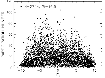
FIG. 1.: Participation numbers versus energy for a 3d system of $14\times 14\times 14=2744$ sites at the Anderson transition.

Diagonalizing the matrix ${\cal H}_{ij}$ for a cubic sample with $N=L^{3}$ sites and open boundary conditions we find a set of $N$ orthonormal eigenvectors $e_{s}(j)$ and corresponding eigenvalues, $E_{j}$. The participation number for a state $j$ is defined as usual by

$${\cal N}_{j}=\left(\sum\limits_{s=1}^{N}e_{s}^{4}(j)\right)^{-1}.$$ (3)

Fig. 1 shows the participation numbers ${\cal N}_{j}$ versus energy $E_{j}$ for a 3d system with $N=2744$ sites. At the transition there is a strong level-to-level fluctuation of the PN. In the whole energy range states are found which are very close in energy but whose ${\cal N}_{j}$ differ by up to two orders of magnitude. This means that the energy of a particular state is not indicative of the spatial behavior of the wave function. In a next step we, therefore, calculate the distribution function of the PN in an energy band around zero energy (where the Anderson transition takes place). We take the width of this band equal $10$ i.e. we include all states with $|E_{j}|<5$. The distribution remains practically the same if we take a much narrower strip, $|E_{j}|<1$ but the computation time increases significantly.

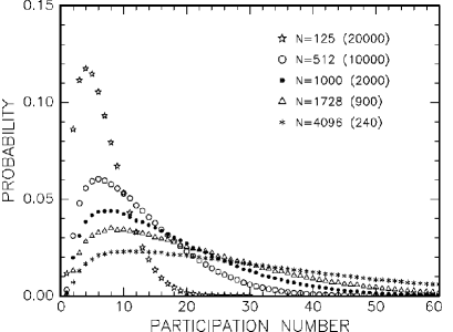
FIG. 2.: Distribution functions of participation numbers at the Anderson transition for different system sizes. In the brackets the numbers of realizations used in the averaging are shown

The normalized distribution functions of the participation numbers for different system sizes are shown in Figure 2. As expected the distributions are strongly size dependent. Increasing the system size the position of the maximum shifts to higher values, approximately as $\propto N^{0.3}$, and the amplitude of the maximum decreases as $\propto N^{-0.46}$.

Let us suppose now that the fluctuation of the PN at the transition is due to fluctuations of $D_{2}$ of the wave functions. According to Eq. (1), without loss of generality, we can take this relation in the form ${\cal N}\propto N^{D_{2}/3}$. Then if $F_{N}({\cal N})$ is the normalized distribution function of PN for an ensemble of systems with $N$ sites and different disorder, we can extract the distribution function of the correlation dimensions, $D_{2}$, in this ensemble

$${\cal P}_{N}(D_{2})=(1/3)F_{N}\left(N^{D_{2}/3}\right)N^{D_{2}/3}\ln N.$$ (4)

Fig. 3 shows that this distribution of correlation dimensions is much less sensitive to the system size than the one of the PN. Moreover, with increasing $N$ it obviously approaches some size independent function, ${\cal P}_{\infty}(D_{2})$, i.e. in the thermodynamic limit a universal distribution function of correlation dimensions does exist at the Anderson transition. For a given model of disorder it should be the same for different realizations. In other words we believe that the distribution function ${\cal P}_{\infty}(D_{2})$ is a self-averaged quantity [16] and can be obtained by analyzing one sufficiently large system.

Fig. 3 shows an additional interesting feature of this distribution: with increasing argument the function ${\cal P}_{N}(D_{2})$ rapidly decays to zero. The drop gets steeper with increasing size $N$. This is seen more clearly in a logarithmic plot of ${\cal P}_{N}(D_{2})$. For systems with $N\geq 512$, ${\cal P}_{N}(D_{2})$ drops four orders of magnitude in the small interval $1.5<D_{2}<2$. We think, therefore, that in the thermodynamic limit there is a point, $D_{\rm 2max}$ where the function ${\cal P}_{\infty}(D_{2})$ approaches exactly zero. In such a case this would be the highest possible value of the correlation dimension $D_{2}$ at the Anderson transition. In the following we present additional evidence in support of this idea.

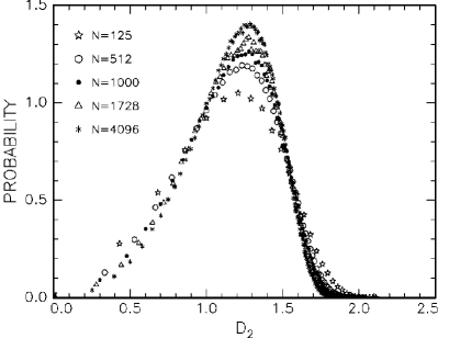
FIG. 3.: Distribution functions of the correlation dimension ${\cal P}_{N}(D_{2})$ at the Anderson transition for different system sizes.

For that purpose we calculate the size dependence of the average PN and of the PN of the the most extended state in the system, i.e. for a given realization of disorder the state with maximal participation number, ${\cal N}_{\rm max}$. The ensemble averages of both quantities (denoted by aapn and ampn, respectively) against system size $N$ are plotted in Fig. 4. First, both quantities scale with $N$ as a power law, $aN^{D_{2}/3}$. Secondly the value $D_{2}=1.26$ for the average participation number (aapn) is very close to the position of the maximum in the distribution function of correlation dimensions shown in Figure 3. It is surprising that averaging over all states does not affect the power law behavior given by Eq. (1) for a single state. For the ensemble average of the maximum participation number, $\left<{\cal N}_{\rm max}\right>$ we find $D_{2}=1.83$. This is the correlation dimension of the most extended state in the system at the transition. To answer the question whether it really is the maximal correlation dimension, $D_{\rm 2max}$, we should study the fluctuations of this quantity. A maximal correlation dimension $D_{\rm 2max}$ does exist if the fluctuation of this quantity goes to zero with $N\to\infty$.

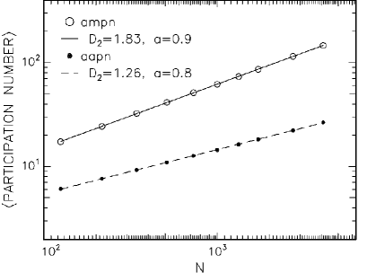
FIG. 4.: Averaged maximum participation number (ampn) and averaged average participation number (aapn) at the transition versus system size. Lines are the best least squares fit with $\left<{\cal N}\right>=aN^{D_{2}/3}$, where $\left<{\cal N}\right>$ is ”ampn” or ”aapn”, respectively.

Fig. 5 shows the relative fluctuations of the maximum participation number versus system size. Firstly the fluctuations are rather small and decrease slowly with increasing $N$. According to Eq. (1) we can relate them to the fluctuations of the correlation dimension $\delta D_{\rm 2max}$

$$\delta_{\rm mpn}\equiv\delta{\cal N}_{\rm max}/\left<{\cal N}_{\rm max}\right>=(\delta D_{\rm 2max}/3)\ln N.$$ (5)

We conclude from the above that, in the thermodynamic limit ($N\to\infty$), the fluctuation of the correlation dimension for the most extended state $\delta D_{\rm 2max}\to 0$ at least not slower than $1/\ln N$. Therefore $D_{\rm 2max}=1.83$ is indeed the highest possible value of the wave function correlation dimension at the Anderson transition. The distribution function ${\cal P}_{\infty}({\cal D}_{2})$ should approach exactly zero at this value.

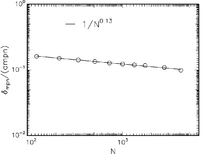
FIG. 5.: Relative root mean square deviation of the maximum participation number against system size. The solid fitting line corresponds to a power law behavior, $\propto 1/N^{0.13}$.

There are numerous previous calculations of the correlation dimension $D_{2}$ at the 3d Anderson transition. From the scaling with system size of the density-density correlation of the wave functions, the correlation dimension was estimated to be $D_{2}=1.7\pm 0.3$ (for $W=16$)[17]. From the size dependence of the participation number averaged, both over different wave functions in a small energy interval $0.25$ around zero and over disorder (with a Gaussian distribution of site energies), the correlation dimension $D_{2}=1.6\pm 0.1$ was estimated[18]. In Ref. [19] from the spectral compressibility, $\chi$ of the levels, using $\chi=(1-D_{2}/d)/2$ derived in Ref. [20] the correlation dimension was estimated as $D_{2}=1.4\pm 0.2$. From the time decay of the temporal autocorrelation function, $C(t)\propto t^{-D_{2}/3}$, the correlation dimension, $D_{2}=1.5\pm 0.2$ was obtained[21]. Using box-counting procedures $D_{2}=1.7\pm 0.2$ [22], $D_{2}=1.52\pm 0.11$ [23], and $D_{2}=1.68$ [24] was calculated. Again using box counting and averaging the results over wave functions in a small energy interval, $\Delta E=0.01$, around zero and over five different realizations of disorder $D_{2}=1.46$ was found [15]. Again using box-counting techniques in Ref. [25], $D_{2}=1.33\pm 0.02$ was obtained.

This shows clearly the quite large uncertainty, in the literature, in the existing values of $D_{2}$ at the transition. The reason is obviously that one deals with a distribution of this quantity. Among different characteristics of this distribution one can consider for example the position of the maximum, at about $1.3$, the average value, $\overline{D_{2}}=1.26$, and the correlation dimension of the most extended state at the transition, $D_{\rm 2max}=1.83$.

Similarly the distribution function of the information dimension $D_{1}$ as well as of the other generalized dimensions $D_{q}$ at the transition can be obtained. The results of this analysis will be published elsewhere. In the thermodynamic limit all these distribution functions are expected to be universal and self-averaged quantities. Using the Legendre transformation the multifractal spectrum $f_{j}(\alpha)$ for each wave function with energy $E_{j}$ can be calculated (compare Ref [26]). In other words critical wave functions at the transition should be characterized by a whole distribution of $f(\alpha)$’s which is already a functional. In particular, the positions of the maxima, $\alpha_{0}$’s of these functions should be distributed.

In conclusion, we investigated numerically the distribution of the correlation fractal dimension $D_{2}$ for the critical wave functions at 3d Anderson transition. This distribution appears to be universal i.e. it no longer depends on the system size in the thermodynamic limit. Extrapolating these results to other fractal dimensions we conclude that each critical wave function should possess its own (infinite) set of generalized fractal dimensions, $D_{d}$ at the transition. And one should rather speak about the distribution functional of these functions.

The authors are very grateful to B.I. Shklovskii for fruitful discussions. One of us (D.A.P.) gratefully acknowledges the financial support and hospitality of the University of Minnesota where part of this work was done.

REFERENCES

- [1] P. A. Lee, T. V. Ramakrishnan, Rev. Mod. Phys, 57, 287 (1985).
- [2] F. Wegner, Z. Phys. B, 36, 209 (1980).
- [3] H. Aoki, J. Phys. C, 16, L205 (1983); Phys.Rev.B, 33, 7310 (1986).
- [4] P. W. Anderson, Phys. Rev. B, 109, 1492 (1958).
- [5] C. Castellani and L. Peliti, J. Phys. A, 19, L429 (1986).
- [6] M. Janssen, Int. J. Mod. Phys. B, 8, 943 (1994).
- [7] V. Fal’ko and K. B. Efetov, Phys. Rev. B, 52, 17413 (1995).
- [8] B. L. Altshuler, V. E. Kravtsov and I. V. Lerner, Phys. Lett. A, 134, 488 (1989).
- [9] S.Yoshino, and M.Okazaki, J.Phys.Soc.Jap, 43, 415 (1977); F.Yonezawa, J. Non-Cryst. Sol., 35&36, 29 (1980).
- [10] In fact it is sufficient that the correlation length was much bigger than the sample size .
- [11] B. Shapiro, Phys.Rev.B, 34, 4394 (1986); Phil. Mag.B, 56, 1031 (1987); Phys. Rev. Lett., 65, 1510 (1990).
- [12] A.Cohen, and B.Shapiro, Int. J. Mod. Phys., 6, 1243 (1992).
- [13] Y.V.Fyodorov, and A.D.Mirlin, Phys. Rev. B, 51, 13403 (1995).
- [14] V. N. Prigodin, and B. L. Altshuler, Phys. Rev. Lett., 80, 1944 (1998).
- [15] H. Grussbach, and M. Schreiber, Phys. Rev. B, 51, 663 (1995).
- [16] To calculate the distribution functions for the rather small sizes shown in Fig. 1 we had, of course, to average over many different realizations of disorder.
- [17] C.M. Soukoulis and E.N. Economou, Phys. Rev. Lett., 52, 565 (1984).
- [18] M. Schreiber, Physica A, 167, 188 (1990).
- [19] D.Braun, G.Montambaux, and M.Pascaud, Phys. Rev. Lett, 81, 1062 (1998).
- [20] J.T. Chalker, V.E. Kravtsov, and I.V. Lerner, JETP Lett., 64, 386 (1996).
- [21] T. Ohtsuki, and T. Kawarabayashi, J. Phys. Soc. Jap., 66, 314 (1997).
- [22] T. Brandes, B. Huckestein, and L. Schwetzer, Ann. Physik, 5, 633 (1996).
- [23] T. Terao, Phys. Rev. B, 56, 975 (1997).
- [24] M. Schreiber, and H. Grussbach, Phys. Rev. Lett, 67, 607 (1991).
- [25] S.N. Evangelou, Physica A, 167, 199 (1990).
- [26] H. Grussbach, and M.Schreiber, Phys. Rev. B, 48, 6650 (1993).