Quantum dot dephasing by edge states

Abstract

We calculate the dephasing rate of an electron state in a pinched quantum dot, due to Coulomb interactions between the electron in the dot and electrons in a nearby voltage biased ballistic nanostructure. The dephasing is caused by nonequilibrium time fluctuations of the electron density in the nanostructure, which create random electric fields in the dot. As a result, the electron level in the dot fluctuates in time, and the coherent part of the resonant transmission through the dot is suppressed.

I Introduction

The dephasing of electron states in Quantum Dots (QD) was considered mainly in connection with weak localization phenomena, see experiments [1, 2] and theory [3, 4]. A different type of phenomenon in which dephasing is important is interference phenomenon in an Aharonov-Bohm ring [5]. If a pinched QD is embedded in one of the arms of such a ring the transmission through this arm is supported by a resonant electron state in the QD. The dephasing of this state [6] suppresses the interference in the ring, and this can be observed as a decrease of of the oscillating part of the ring conductance [7].

The dephasing is due to electron-phonon or electron-electron interactions of the QD electrons with some “environment”, which can either be in equilibrium or driven out of it by external forces. In the experiment [7] the dephasing was due to the capacitive interaction of the QD with a voltage biased point contact (PC), and the amount of dephasing was dependent on the bias. In a situation like this one can separate the equilibrium dephasing, which depends only on the temperature of the environment, from an additional dephasing which is due to voltages applied to the environment. The theory concerning this experiment was given in [6, 8].

In recent experiments [9] the nanostructure (NS), that was capacitively coupled to the QD, was a multiterminal 2DEG device in a quantizing magnetic field . We present in this paper a generalization of the theory given in [6] that takes into account the specific effects appearing due to the complicated geometry, and the chirality of the states in the NS (see Fig.1). A similar problem was addressed in [10] using a different approach, based on lumped mesoscopic circuit elements. Broadening of electron transitions in self-assembled QD’s due to Coulomb interactions with the electrons in the wetting layer was considered in [11].

II Model

We consider a QD with a single level $\epsilon_{0}$, that is described by the Hamiltonian $H_{QD}=\epsilon_{0}c^{+}c$, where $c^{+}$ is an operator creating an electron in the QD state. The NS is a multiterminal junction in the 2DEG described by the Hamiltonian

$$H_{NS}=\int d{\bf r}\Psi^{+}({\bf r})H({\bf r})\Psi({\bf r}),\qquad H({\bf r})={1\over 2m}\left(-i\nabla-{e\over c}{\bf A}({\bf r})\right)^{2}+U({\bf r}),$$ (1)

where $U({\bf r})$ is the potential confining the 2DEG, ${\bf A}({\bf r})$ is the vector potential of the external magnetic field $(e<0,\hbar=1)$, and $\Psi({\bf r})$ is the electron field operator. The capacitive interaction between the QD and the NS, assumed to be weak, is

$$H_{int}=c^{+}c\int d{\bf r}W({\bf r})\rho({\bf r}),$$ (2)

where $\rho({\bf r})=\Psi^{+}({\bf r})\Psi({\bf r})$ is the electron density operator, and $W({\bf r})$ is a Coulomb interaction kernel.

The perturbation Eq.(2) has a “dual” meaning. If one combines $H_{NS}+H_{int}$ one can see that $W({\bf r})$ is the change of the confining potential $U({\bf r})$ due to one electron occupying the QD state (when $<c^{+}c>=1$), while combining $H_{QD}+H_{int}$ one can see that $\int d{\bf r}W({\bf r})\rho({\bf r})$ is the change of the energy $\epsilon_{0}$ due to the Coulomb interaction of the electron in the QD with the electron density in the NS.

III Dephasing rate notion

At low temperatures the dephasing is due to electron-electron interactions [12]. To calculate the dephasing rate we use the method developed in [6]. The electron density in the NS fluctuates in time and creates a fluctuating potential in the QD which brings about fluctuations of the energy level $\epsilon_{0}$. These fluctuations are given by

$$\delta\epsilon_{0}(t)=\int d{\bf r}W({\bf r})\delta\rho({\bf r},t),$$ (3)

where $\delta\rho({\bf r},t)\equiv\rho({\bf r},t)-\langle\rho({\bf r})\rangle$. As a result, the correlator $\langle\delta\epsilon_{0}(t)\delta\epsilon_{0}(0)\rangle$ is defined by the density-density correlator $\langle\delta\rho({\bf r},t)\delta\rho({\bf r}^{\prime},0)\rangle$, while $\langle\delta\epsilon_{0}\rangle=0$.

Consider resonant transmission through the QD for electron energies $\epsilon$ close to $\epsilon_{0}$. When the QD level does not fluctuate the transmission amplitude $t(\epsilon)$ contains the Breit-Wigner factor $-i/[(\epsilon-\epsilon_{0})+i\Gamma]$, where $\Gamma$ is the width of the level due to the QD’s connection with the leads. When the level fluctuates the transmission and reflection can be elastic and inelastic. In interference experiments only the elastic transmission is of importance and to obtain the elastic transmission amplitude $\langle t(\epsilon)\rangle$ one has to replace the Breit-Wigner factor by [6]

$$\int_{0}^{\infty}dt\exp[-\Gamma t-\Phi(t)+i(\epsilon-\epsilon_{0})t],$$ (4)

where

$$\Phi(t)={1\over 2}\int_{0}^{t}dt^{\prime}\int_{0}^{t}dt^{\prime\prime}\langle\delta\epsilon_{0}(t^{\prime})\delta\epsilon_{0}(t^{\prime\prime})\rangle.$$ (5)

One can see that $|\langle t(\epsilon)\rangle|<|t(\epsilon)|$ which means dephasing of the QD state, that is responsible for resonant transmission. The same can be understood from the dynamics of the QD state amplitude [6], $\langle c(t)^{+}c(0)\rangle=\langle c(0)^{+}c(0)\rangle\exp[i\epsilon_{0}t-\Gamma t-\Phi(t)].$

The level fluctuations are characterized by their amplitude $\langle(\delta\epsilon_{0})^{2}\rangle^{1/2}$ and by the correlation time $\tau_{c}$. The amplitude is proportional to the strength of the capacitive coupling $W$, while the correlation time is independent of $W$ and is determined by the correlation time of the density-density correlator. Hence, for weak enough coupling, one has $\langle(\delta\epsilon_{0})^{2}\rangle^{1/2}\tau_{c}\ll 1$, which corresponds to dynamical narrowing. In this case $\Phi(t)=\gamma t$ and the integral Eq.(4) reduces to $-i/[(\epsilon-\epsilon_{0})+i(\Gamma+\gamma)]$. Here

$$\gamma=\pi K(0),$$ (6)

with the following level oscillations’ spectrum

$$K(\omega)={1\over 2\pi}\int_{-\infty}^{+\infty}dte^{i\omega t}\langle\delta\epsilon_{0}(t)\delta\epsilon_{0}(0)\rangle.$$ (7)

This result means that in the case of dynamical narrowing one can describe the dephasing by a dephasing time $\tau_{\varphi}=\gamma^{-1}$. The dephasing rate can be estimated as $\gamma\simeq\langle(\delta\epsilon_{0})^{2}\rangle\tau_{c}$, and is smaller than the amplitude of the level fluctuations $\langle(\delta\epsilon_{0})^{2}\rangle^{1/2}$. In the general case when $\langle(\delta\epsilon_{0})^{2}\rangle^{1/2}\tau_{c}\gtrsim 1$, the transmission probability $|\langle t(\epsilon)\rangle|^{2}$ is not a Lorenzian, and a dephasing time can not be defined.

IV Dephasing rate calculation

To calculate the correlator $K(\omega)$ we represent the field operator in terms of scattering states (SS’s) [14] (see Appendix)

$$\Psi({\bf r})=\int{d\epsilon\over 2\pi}\sum_{\alpha n}a_{\alpha n}(\epsilon)\chi_{\alpha n}(\epsilon,{\bf r}),$$ (8)

where $a_{\alpha n}^{+}(\epsilon)$ is an operator creating an incoming electron in channel $n$ of terminal $\alpha$, with energy $\epsilon$. Performing calculations similar to those in [6] we find

$$K(\omega)=\sum_{\alpha\alpha^{\prime}}K^{\alpha\alpha^{\prime}}(\omega),$$ (9)

where the contribution from terminals $\alpha$ and $\alpha^{\prime}$ is

$$K^{\alpha\alpha^{\prime}}(\omega)={1\over 2}\int{d\epsilon\over 2\pi}\int{d\epsilon^{\prime}\over 2\pi}\sum_{nn^{\prime}}f_{\alpha}(\epsilon)[1-f_{\alpha^{\prime}}(\epsilon^{\prime})]|W_{\alpha n,\alpha^{\prime}n^{\prime}}(\epsilon,\epsilon^{\prime})|^{2}[\delta(\epsilon^{\prime}-\epsilon-\omega)+\delta(\epsilon^{\prime}-\epsilon+\omega)].$$ (10)

Here we used the fact that when the SS’s are normalized to a unit of incoming flux one has $\langle a^{+}_{\alpha n}(\epsilon)a_{\alpha^{\prime}n^{\prime}}(\epsilon^{\prime})\rangle=2\pi\delta(\epsilon-\epsilon^{\prime})\delta_{\alpha n,\alpha^{\prime}n^{\prime}}f_{\alpha}(\epsilon)$, where $f_{\alpha}(\epsilon)$ is the Fermi distribution for energy $\epsilon$ in terminal $\alpha$. It is convenient to write it as $f(\epsilon-\delta\mu_{\alpha})$, where $\delta\mu_{\alpha}=\mu_{\alpha}-\mu$ and $f(\epsilon)=\left(e^{(\epsilon-\mu)/T}+1\right)^{-1}$ is the Fermi distribution with some reference chemical potential $\mu$. The matrix element entering Eq.(10) contains SS’s,

$$W_{\alpha n,\alpha^{\prime}n^{\prime}}(\epsilon,\epsilon^{\prime})=\int d{\bf r}W({\bf r})\chi_{\alpha n}(\epsilon,{\bf r})^{*}\chi_{\alpha^{\prime}n^{\prime}}(\epsilon^{\prime},{\bf r}).$$ (11)

The integration here is over the interaction area, i.e. over that part of the NS which is close enough to the QD and where $W({\bf r})$ is not small (see Fig.1).

In what follows we consider the case when the voltages $V_{\alpha}$ applied to all terminals are small. We choose $\mu$ to be the equilibrium chemical potential (when all $V_{\alpha}=0$) and $\delta\mu_{\alpha}=eV_{\alpha}$. In this case the relevant energies in Eq.(10) correspond to the small energy window $|\epsilon-\mu|\lesssim\max[T,eV]$, where electron exchange between terminals happens. We assume that within this energy window one can neglect the energy dependence of the scattering states and hence of the matrix elements Eq.(11). As a result we have

$$K^{\alpha\alpha^{\prime}}(\omega)={1\over 2}|W_{\alpha,\alpha^{\prime}}|^{2}\int{d\epsilon\over 2\pi}\int{d\epsilon^{\prime}\over 2\pi}f(\epsilon-eV_{\alpha})[1-f(\epsilon^{\prime}-eV_{\alpha^{\prime}})][\delta(\epsilon^{\prime}-\epsilon-\omega)+\delta(\epsilon^{\prime}-\epsilon+\omega)],$$ (12)

with an effective matrix element

$$|W_{\alpha,\alpha^{\prime}}|^{2}\equiv\sum_{nn^{\prime}}|W_{\alpha n,\alpha^{\prime}n^{\prime}}|^{2}.$$ (13)

Shifting the integration variables in Eq.(12) by $eV_{\alpha}$ and $eV_{\alpha^{\prime}}$ one can see that the diagonal contributions $K^{\alpha\alpha}$ do not depend on the applied voltages $V_{\alpha}$, and are equal to their equilibrium values at $V_{\alpha}=0$, i.e.

$$K^{\alpha\alpha}(\omega)={1\over 8\pi^{2}}|W_{\alpha,\alpha}|^{2}F_{T}(\omega),$$ (14)

where $F_{T}(\omega)=\omega\coth(\omega/2T)=2\omega\left[N_{T}(\omega)+{1\over 2}\right]$, with $N_{T}(\omega)=\left(e^{\omega/T}+1\right)^{-1}$. Note that $F_{T}(0)=2T$ and $F_{0}(\omega)=|\omega|$.

For the nondiagonal contributions $\alpha\neq\alpha^{\prime}$ we find after a shift of the integration variables

$$K^{(\alpha\alpha^{\prime})}(\omega)\equiv K^{\alpha\alpha^{\prime}}(\omega)+K^{\alpha^{\prime}\alpha}(\omega)={1\over 8\pi^{2}}|W_{\alpha,\alpha^{\prime}}|^{2}[F_{T}(\omega+eV_{\alpha\alpha^{\prime}})+F_{T}(\omega-eV_{\alpha\alpha^{\prime}})],$$ (15)

where $V_{\alpha\alpha^{\prime}}=V_{\alpha}-V_{\alpha^{\prime}}$.

Using Eq.(9) one can find the dephasing rate as a sum over single terminals and pairs of terminals,

$$\gamma=\sum_{\alpha}\gamma^{(\alpha)}+\sum_{\alpha<\alpha^{\prime}}\gamma^{(\alpha\alpha^{\prime})}.$$ (16)

It follows from Eq.(14) that a single terminal contributes to the dephasing only if SS’s emitted from this terminal reach the interaction area, and that this is always an equilibrium contribution,

$$\gamma^{(\alpha)}=\pi K^{\alpha\alpha}(0)={1\over 4\pi}|W_{\alpha,\alpha}|^{2}T.$$ (17)

A pair of terminals contribute to the dephasing only if SS’s emitted from both terminals overlap in the interaction area,

$$\gamma^{(\alpha\alpha^{\prime})}=K^{(\alpha\alpha^{\prime})}(0)={1\over 4\pi}|W_{\alpha,\alpha^{\prime}}|^{2}F_{T}(eV_{\alpha\alpha^{\prime}}).$$ (18)

When both terminals are at the same voltage, the contribution of this pair to dephasing is an equilibrium one.

Note that $F_{T}(\omega)$ contains the “zero point fluctuations”, but they do not contribute to the equilibrium dephasing rate, given by $K(\omega)$ at $\omega=0$, hence for zero temperature there is no equilibrium dephasing.

If one is interested in nonequilibrium dephasing one has to look only at pairs of terminals which are at different voltages, and which send scattering states that overlap in the interaction region. The nonequilibrium contribution of such a pair is

$$\gamma^{(\alpha\alpha^{\prime})}_{V}\equiv\gamma^{(\alpha\alpha^{\prime})}-\gamma^{(\alpha\alpha^{\prime})}|_{V=0}={1\over 4\pi}|W_{\alpha,\alpha^{\prime}}|^{2}[F_{T}(eV_{\alpha\alpha^{\prime}})-F_{T}(0)].$$ (19)

For zero temperature it reduces to

$$\gamma^{(\alpha\alpha^{\prime})}_{V}|_{T=0}={1\over 4\pi}|W_{\alpha,\alpha^{\prime}}|^{2}|eV_{\alpha\alpha^{\prime}}|.$$ (20)

Using the dual property of the interaction between the QD and the NS, we consider now $W({\bf r})$ as a small variation of the confining potential $U({\bf r})$ due to an electron occupying the QD. As a result the scattering matrix of the NS is changed according to Eq.(46) from $S$ to $S+\delta S$. Using in addition Eq.(37) we can express the matrix elements Eq.(11) in terms of the scattering matrix variation

$$W_{\alpha n\epsilon,\alpha^{\prime}n^{\prime}\epsilon}=i\sum_{\beta m}S_{\beta m,\alpha n}(\epsilon)^{*}\delta S_{\beta m,\alpha^{\prime}n^{\prime}}(\epsilon).$$ (21)

Pinching the QD to the Coulomb blockade regime one can change the number of electrons in the QD one by one and measure the variation of the conductance matrix $G_{\beta\alpha}$ due to an additional electron in the QD [13]. Since $G_{\beta\alpha}=\sum_{mn}|S_{\beta m,\alpha n}|^{2}-\delta_{\beta,\alpha}$, this is a way to measure (in case of simple enough NS geometry) the variation $\delta S$ and the matrix elements $W$. This procedure was performed experimentally [7] for the simplest NS, being a one channel point contact.

V Dephasing versus current noise

Dephasing is closely related to current noise since current fluctuations are related to charge density fluctuations by the continuity equation. The results obtained in [14] for the current noise can be presented in the following form

$$\langle\delta I_{\alpha}\delta I_{\alpha^{\prime}}\rangle={e^{2}\over 8\pi^{2}}\sum_{\beta\beta^{\prime}}A_{\beta\beta^{\prime}}^{\alpha\alpha^{\prime}}F_{T}(eV_{\beta\beta^{\prime}}).$$ (22)

Here the left hand side is the $\omega=0$ Fourier component of the current cross-correlator in terminals $\alpha$ and $\alpha^{\prime}$,

$$A_{\beta\beta^{\prime}}^{\alpha\alpha^{\prime}}=\sum_{mm^{\prime}}A^{\alpha}_{\beta m,\beta^{\prime}m^{\prime}}A^{\alpha^{\prime}}_{\beta^{\prime}m^{\prime},\beta m},$$ (23)

with

$$A^{\alpha}_{\beta m,\beta^{\prime}m^{\prime}}=\delta_{\beta\alpha}\delta_{\beta^{\prime}\alpha}\delta_{mm^{\prime}}-\sum_{n}S^{*}_{\alpha n,\beta m}S_{\alpha n,\beta^{\prime}m^{\prime}},$$ (24)

where the scattering matrix is at $\epsilon=\mu$. One can see that a single terminal $\beta$ contributes to $\langle\delta I_{\alpha}\delta I_{\alpha^{\prime}}\rangle$ only if SS’s emitted from this terminal reach both terminals $\alpha$ and $\alpha^{\prime}$, and that this contribution, given by the term with $\beta^{\prime}=\beta$ is always equilibrium. Pairs of terminals $\beta$ and $\beta^{\prime}$ contribute to $\langle\delta I_{\alpha}\delta I_{\alpha^{\prime}}\rangle$ only if SS’s emitted from each of these terminals reach both terminals $\alpha$ and $\alpha^{\prime}$. This contribution given by terms with $\beta^{\prime}\neq\beta$ contains a nonequilibrium part. These conditions are very similar to those in case of dephasing.

VI Examples and discussion

We consider first a simple one channel 2-terminal device with a gate and a QD (see Fig.2). The scattering matrix of the gate (in the absence of an electron in the QD) is

$$S=\left|\begin{array}[]{cc}r&{\tilde{t}}\\ t&{\tilde{r}}\end{array}\right|\equiv\left|\begin{array}[]{cc}\cos\theta e^{i\alpha}&\sin\theta e^{i{\tilde{\beta}}}\\ \sin\theta e^{i\beta}&\cos\theta e^{i{\tilde{\alpha}}}\end{array}\right|,\qquad{\tilde{\alpha}}-{\tilde{\beta}}=\pi-(\alpha-\beta),$$ (25)

where $r$ and $t$ correspond to reflection and transmission of the SS’s approaching the gate from left, while ${\tilde{r}}$ and ${\tilde{t}}$ correspond to the SS’s approaching the gate from the right. If the magnetic field $B\neq 0$ the scattering matrix is not symmetric, $t\neq{\tilde{t}}$.

In case of zero temperature the equilibrium part of the QD state dephasing rate vanishes, and the nonequilibrium part is according to Eq.(20) and Eq.(21)

$$\gamma=\pi|W|^{2}eV,\qquad\qquad|W|^{2}=|r^{*}\delta{\tilde{t}}+t^{*}\delta{\tilde{r}}|^{2}=|\delta\theta-i(\delta\beta-\delta\alpha)\sin\theta\cos\theta|^{2}.$$ (26)

Here $V\equiv|V_{12}|$ and $\delta{\tilde{t}}$ , $\delta{\tilde{r}}$ are the changes of the transmission and the reflection amplitudes due to the electron in the QD. This result was obtained in [6] for $B=0$ and a symmetric gate. The shot noise in this device (in the absence of an electron in the QD) is [15]

$$\langle(\delta I)^{2}\rangle=(e^{2}/4\pi^{2})|r|^{2}|t|^{2}eV.$$ (27)

Both the dephasing and the shot-noise are due to the same nonequilibrium fluctuations, but they are not proportional to each other. To get some insight, consider first zero or a weak magnetic field, when both SS’s 1 and 2 occupy the whole crossection of the sample (see Fig. 2). If we assume there is no reflection from the gate, i.e. $|t|^{2}=1$, $|r|^{2}=0$, we find $\langle(\delta I)^{2}\rangle=0$, while $\gamma=\pi|\delta r|^{2}eV\neq 0$. The dephasing is nonzero because SS’s emitted from different terminals overlap near the QD, while the shot noise is zero because each terminal (where the shot noise is measured) is feeded only by one SS. The situation for the shot noise changes if the gate is reflecting, in which case each terminal is feeded by both SS’s.

One can understand this difference from the following simple calculation. In a channel without reflection the wave function is $\psi(x)=ae^{ikx}+be^{-ikx}$, where the two terms are SS’s coming from the left and right terminals. The corresponding charge and current densities are $\rho(x)=e\{|a|^{2}+|b|^{2}+(ab^{*}e^{i2kx}+c.c.)\}$ and $j(x)=ev_{k}\{|a|^{2}-|b|^{2}\}$. What is important for nonequilibrium fluctuations is the overlap of SS’s coming from different terminals, i.e. terms proportional to $ab$. Such terms do not exist in $j$ but do exist in $\rho$. This is why the shot-noise is zero, while the dephasing rate is not. The term $(ab^{*}e^{i2kx}+c.c.)$ is of quantum origin. It means that in a quasiclassical situation, when the number of channels is large, this term will average out due to “integration” over $k$. When the gate is reflecting, $|t|^{2}\neq 1$, $|r|^{2}\neq 0$, both $\rho(x)$ and $j(x)$ contain terms proportional to $ab$. One can easily check it using, for example, the wave function to the left of the barrier $\psi(x)=a[e^{ikx}+re^{-ikx}]+b{\tilde{t}}e^{-ikx}$. It is also important to notice that for $\omega=0$ the current and charge fluctuations are not coupled by the continuity equation.

Consider now the same device in a strong magnetic field when the SS’s are edge states (ES’s) localized near the boundaries. We assume also that the QD is far from the gate and the interaction region does not reach ES2. In this situation due to the chirality of ES1 the QD can change only the phases of $t$ and ${\tilde{r}}$. As a result $|W|^{2}=(\delta\beta)^{2}|t|^{2}|r|^{2}$, i.e. the dephasing rate is proportional to the shot-noise. This is because for chiral states the current and charge densities are proportional, $j=\rho v_{k}$. (The connection between dephasing and the phase of $t$ was mensioned in [16]).

As a second example we consider a 4-terminal device similar to that used in experiment [9], with a geometry as shown in Fig.3. The source S ($\alpha=1$) and the drain D ($\alpha=2$) are used to bias the device. Two floating terminals, one down-stream from S to D ($\alpha=3$) and one up-stream from D to S ($\alpha=4$) are “dephasors” according to [17]. Gate A regulates the source-drain current, while gates B and C block the floating terminals. The QD is located far from gate B. We assume there is only one LL at the Fermi energy and that the ES’s at opposite edges are well separated and do not overlap. We will be interested only in nonequilibrium dephasing and consider zero temperature.

The SS’s emitted from the up-stream floating terminal 4 do not reach the interaction region and hence this terminal does not contribute to the dephasing of the QD. (In what follows it is assumed that this terminal is blocked). Only scattering states emitted from terminals 1,2, and 3 overlap in the interaction region, and hence in accordance with Eq.(16) one has $\gamma=\gamma^{(12)}+\gamma^{(23)}+\gamma^{(31)}.$ Since the QD is located far from point contact B, all SS’s in the interaction region have the form of the same ES $w^{-}_{2}({\bf r})\equiv w({\bf r})$ with different amplitudes, i.e. $\chi_{1}=e^{i\phi_{1}}t_{A}r_{B}w,\;\chi_{2}=e^{i\phi_{2}}{\tilde{r}}_{A}r_{B}w,\;\chi_{3}=e^{i\phi_{3}}{\tilde{t}}_{B}w.$ Here $r_{A}$, $t_{A}$ and ${\tilde{r}}_{A}$, ${\tilde{t}}_{A}$ are the reflection and transmission amplitudes for ES’s approaching A from left and from right. $r_{B}$, $t_{B}$ and ${\tilde{r}}_{B}$, ${\tilde{t}}_{B}$ correspond to ES’s approaching B from above and below. The phase factors $e^{i\phi}$ depend on the position of the QD. The relevant matrix elements Eq.(13) are

$$|W_{12}|^{2}=|t_{A}r_{B}|^{2}|r_{A}r_{B}|^{2}|W|^{2},\;|W_{13}|^{2}=|t_{B}|^{2}|t_{A}r_{B}|^{2}|W|^{2},\;|W_{23}|^{2}=|t_{B}|^{2}|r_{A}r_{B}|^{2}|W|^{2},$$ (28)

where

$$W=\int d{\bf r}W({\bf r})|w({\bf r})|^{2}.$$ (29)

Using these matrix elements we find

$$\gamma^{(12)}=A|t_{A}|^{2}|r_{A}|^{2}|r_{B}|^{4}|V_{12}|,\;\gamma^{(23)}=A|t_{B}|^{2}|r_{B}|^{2}|r_{A}|^{2}|V_{23}|,\;\gamma^{(31)}=A|t_{B}|^{2}|r_{B}|^{2}|t_{A}|^{2}|V_{13}|,$$ (30)

with the constant $A=(e/4\pi)|W|^{2}$.

When terminal 3 is open, i.e. $r_{B}=0$, SS1 and SS2 are absorbed in this terminal and then the interaction region is reached only by SS3. There is no overlap in the interaction region of SS’s emitted from different terminals and as a result all the contributions to nonequilibrium dephasing rate vanish. When terminal 3 is blocked, i.e. $t_{B}=0$ we find $\gamma=\gamma^{(12)}=A|t_{A}|^{2}|r_{A}|^{2}|V_{12}|\equiv\gamma_{0}$.

Since terminal 3 is floating $V_{3}$ is given by the condition that the current entering this terminal is zero, which leads to $V_{3}=V_{1}|t_{A}|^{2}+V_{2}|r_{A}|^{2}$. Using this one finds

$$\gamma=\gamma_{0}\;|r_{B}|^{2}\;(2-|r_{B}|^{2}).$$ (31)

One can see from this result that $\gamma<\gamma_{0}$, i.e. the floating terminal suppresses the nonequilibrium dephasing rate of the QD state. This result is in agreement with experiment [9]. We would like to stress that the suppression is not because of dephasing the SS’s coming to the interaction region. The absolute values of the matrix elements that enter the expression of the dephasing rate according to Eq.(20) do not depend on the phases of the SS’s overlapping in the interaction region. If one would simply destroy their phases it would not affect the dephasing rate $\gamma$. The floating terminal suppresses $\gamma$ because it absorbs the SS’s moving towards the interaction region from different terminals. It is important to have in mind that a theory based on the representation Eq.(8) assumes that terminals absorb incoming waves as black bodies, which means that terminals have infinite capacitance.

It is instructive to compare the dephasing rate with the shot noise. When terminal 3 is blocked the shot noise is known to be $\langle(\delta I_{1})^{2}\rangle=\langle(\delta I_{2})^{2}\rangle=(e^{2}/4\pi^{2})e|V_{12}||t_{A}|^{2}|r_{A}|^{2}.$ Using Eq.(36) one can see that opening terminal 3 does not change $\langle(\delta I_{1})^{2}\rangle$ but suppress $\langle(\delta I_{2})^{2}\rangle$ by exactly the same factor $|r_{B}|^{2}(2-|r_{B}|^{2})$ as the dephasing rate.

Acknowlegements

I am thankful to Y.Imry and B.Spivak for valuable discussions. I also thank M.Heiblum and D.Shprinzak who informed me about their recent unpublished experiments. The work was supported by the Israel Academy of Sciences and Humanities and Ministry of Science of Israel.

In this Appendix we list some useful properties of the Green function, the scattering states and the scattering matrix, valid also when the magnetic field $B\neq 0$.

For each terminal $\alpha$, and given energy $\epsilon$ we define outgoing waves $w_{\alpha n}^{+}(\epsilon,{\bf r})$ and incoming waves $w_{\alpha n}^{-}(\epsilon,{\bf r})$, where $n$ is the mode number (see Fig.1). In case of a strong magnetic field $w^{\pm}$ are ES’s and $n$ is the LL number. The waves $w^{\pm}$ are normalized to carry a unit flux over the cross section of the terminal. Choosing the gauge $A_{x}=-By,A_{y}=0$ for a given terminal, where $x$ and $y$ are the longitudinal and transverse coordinates in this terminal, one can represent the waves as follows: $w_{n}^{+}(\epsilon,{\bf r})=\exp[ik_{n}^{+}(\epsilon)x]\phi_{n}^{+}(\epsilon,y),\;\;w_{n}^{-}(\epsilon,{\bf r})=\exp[ik_{n}^{-}(\epsilon)x]\phi_{n}^{-}(\epsilon,y)$.

In what follows we use “hat” to indicate the magnetic field inversion. It means for example that if $w^{+}_{n}$ is an outgoing wave for the field $B$ (i.e. an outgoing ES for LL $n$) then ${\hat{w}}^{+}_{n}$ is an outgoing wave for field $-B$ (i.e. an outgoing ES for the same LL near the opposite boundary). It is easy to check that $w_{\alpha n}^{\pm}(\epsilon,{\bf r})^{*}={\hat{w}}_{\alpha n}^{\mp}(\epsilon,{\bf r})$ or equivalently $k_{n}^{\pm}(\epsilon)=-{\hat{k}}_{n}^{\mp}(\epsilon)$ and $\phi_{n}^{\pm}(\epsilon,y)={\hat{\phi}}_{n}^{\mp}(\epsilon,y)^{*}$.

Different functions $\phi(y)$ corresponding to the same wave vector $k$ are eigenfunctions of the same Hamiltonian and are orthogonal. This is not the case when two functions $\phi_{1}(y)$ and $\phi_{2}(y)$ correspond to the same energy $\epsilon$, but to different wave vectors $k_{1}$ and $k_{2}$. In this case the “orthogonality” relations are [18]

$$\int dy\phi_{1}\phi_{2}[(k_{1}-{e\over c}A_{x})+(k_{2}-{e\over c}A_{x})]=0,$$ (32)

and

$$\int dy\phi_{1}{\hat{\phi}}_{2}[(k_{1}-{e\over c}A_{x})-(k_{2}+{e\over c}A_{x})]=0.$$ (33)

For a given energy $\epsilon$ the incoming field in terminal $\alpha$ is a superposition of incoming waves $\sum_{n}a_{\alpha n}(\epsilon)w_{\alpha n}^{-}(\epsilon,{\bf r}),$ while the outgoing field in terminal $\beta$ is a superposition of outgoing waves $\sum_{m}b_{\beta m}(\epsilon)w_{\beta m}^{+}(\epsilon,{\bf r}).$ The scattering matrix connects the amplitudes of the incoming and outgoing waves

$$b_{\beta m}(\epsilon)=\sum_{\alpha n}S_{\beta m,\alpha n}(\epsilon)a_{\alpha n}(\epsilon).$$ (34)

The scattering matrix is unitary due to flux conservation

$$\sum_{\beta m}S_{\beta m,\alpha n}(\epsilon)^{*}S_{\beta m,\alpha^{\prime}n^{\prime}}(\epsilon)=\delta_{\alpha n,\alpha^{\prime}n^{\prime}},$$ (35)

and due to time reversal

$$S_{\beta m,\alpha n}(\epsilon)={\hat{S}}_{\alpha n,\beta m}(\epsilon).$$ (36)

A scattering state $\chi_{\alpha n}(\epsilon,{\bf r})$ is defined as a solution of the Schroedinger equation with energy $\epsilon$ excited by an incoming wave $w_{\alpha n}^{-}(\epsilon,{\bf r})$. Complex conjugate scattering states are solutions of the Schroedinger equation with inverted magnetic field. Comparing the behaviour of $\chi^{*}$ and ${\hat{\chi}}$ at infinity one finds that

$$\chi_{\alpha n}(\epsilon,{\bf r})^{*}=\sum_{\beta m}S_{\beta m,\alpha n}(\epsilon)^{*}\;{\hat{\chi}}_{\beta m}(\epsilon,{\bf r})$$ (37)

and also

$${\hat{\chi}}_{\alpha n}(\epsilon,{\bf r})=\sum_{\beta m}{\hat{S}}_{\beta m,\alpha n}(\epsilon)\;\chi_{\beta m}(\epsilon,{\bf r})^{*}.$$ (38)

The Green function is defined by the equation

$$[H({\bf r})-\epsilon]G_{\epsilon}({\bf r},{\bf r}^{\prime})=-\delta({\bf r}-{\bf r}^{\prime}),$$ (39)

with the Hamiltonian given by Eq.(1). The boundary conditions are $G_{\epsilon}({\bf r},{\bf r}^{\prime})=0$ when ${\bf r}$ is at the boundary of the NS, and these correspond to outgoing waves when ${\bf r}$ approaches infinity in some of its terminals. The Green theorem in case $B\neq 0$ is as follows [19]

$$\int({\bf r})(uHv-vH^{*}u)=-{i\over 2m}\oint dl\;{\bf n}\left[u(-i\nabla-{e\over c}{\bf A})v-v(-i\nabla+{e\over c}{\bf A})u\right],$$ (40)

where ${\bf n}$ is the unit normal vector directed outside the NS, $dl$ is an element of the boundary.

Using this theorem and Eq.(33) one can prove the symmetry $G_{\epsilon}({\bf r}^{\prime},{\bf r})={\hat{G}}_{\epsilon}({\bf r},{\bf r}^{\prime}).$

When ${\bf r}$ approaches infinity in terminal $\beta$

$$\chi_{\alpha n}(\epsilon,{\bf r})|_{{\bf r}\rightarrow\infty\beta}=\delta_{\alpha\beta}w_{\alpha n}^{-}(\epsilon,{\bf r})+\sum_{m}S_{\beta m,\alpha n}(\epsilon)w_{\beta m}^{+}(\epsilon,{\bf r}),$$ (41)

and

$$G_{\epsilon}({\bf r},{\bf r}^{\prime})|_{{\bf r}\rightarrow\infty\beta}=-i\sum_{m}w_{\beta m\epsilon}^{+}({\bf r}){\hat{\chi}}_{\beta m\epsilon}({\bf r}^{\prime}).$$ (42)

The first equation follows from the definition of the scattering states and the scattering matrix, while the second equation can be obtained as follows. From the explicit expression of the Green function for a waveguide in a magnetic field given in [20] one can see that a unit source $-\delta({\bf r}-{\bf r}^{\prime})$ at ${\bf r}^{\prime}\rightarrow\infty\beta$ excites an incoming field $-i\sum_{m}w^{-}_{\beta m}(\epsilon,{\bf r}^{\prime})^{*}w^{-}_{\beta m}(\epsilon,{\bf r}).$ Since each wave $w^{-}_{\beta m}(\epsilon,{\bf r})$ excites a state $\chi_{\beta m}(\epsilon,{\bf r})$ we find that

$$G_{\epsilon}({\bf r},{\bf r}^{\prime})|_{{\bf r}^{\prime}\rightarrow\infty\beta}=-i\sum_{m}w^{-}_{\beta m}(\epsilon,{\bf r}^{\prime})^{*}\chi_{\beta m}(\epsilon,{\bf r}).$$ (43)

Using the symmetry of $G$, and the relation between $w^{-}$ and $w^{+}$, we find the relation given above.

A useful function is defined as follows

$$G_{\epsilon}({\bf r},{\bf r}^{\prime})-{\hat{G}}_{\epsilon}({\bf r},{\bf r}^{\prime})^{*}\equiv-ig_{\epsilon}({\bf r},{\bf r}^{\prime}).$$ (44)

This function can be presented in terms of the scattering states

$$g_{\epsilon}({\bf r},{\bf r}^{\prime})=\sum_{\alpha n}\chi_{\alpha n\epsilon}({\bf r})\chi_{\alpha n\epsilon}({\bf r}^{\prime})^{*}.$$ (45)

Obviously $g_{\epsilon}({\bf r},{\bf r})$ is the local density of states. Inverting $B$ one finds ${\hat{g}}_{\epsilon}({\bf r},{\bf r}^{\prime})=g_{\epsilon}({\bf r},{\bf r}^{\prime})^{*}.$ For $B=0$ the function $g_{\epsilon}({\bf r},{\bf r}^{\prime})$ is real.

Let the confining potential $U({\bf r})$ be subjected to some variation $\delta U({\bf r})$. The variation of the scattering states $\delta\chi_{\alpha m}(\epsilon,{\bf r})$ contains only outgoing waves and can be found from the first Born approximation using the retarded Green function corresponding to the potential $U({\bf r})$. The asymptotic behaviour of $\delta\chi_{\alpha m}(\epsilon,{\bf r})$ at ${\bf r}\rightarrow\infty\beta$ can then be found using Eq.(42). As a result the variation of the scattering matrix is

$${\delta\over\delta U({\bf r})}S_{\alpha n,\beta m}(\epsilon)=-i{\hat{\chi}}_{\alpha n}(\epsilon,{\bf r})\chi_{\beta m}(\epsilon,{\bf r}).$$ (46)

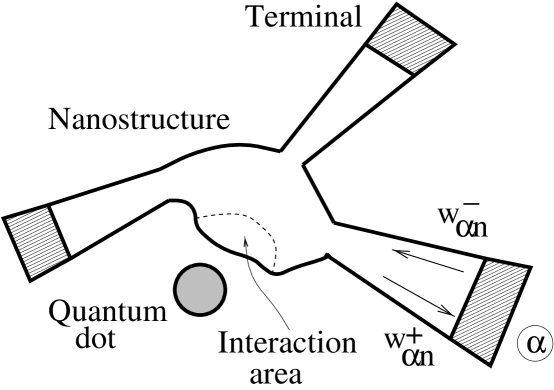
FIG. 1.: The quantum dot and the nanostructure. $w^{\pm}_{\alpha n}$ are waves emitted and absorbed by terminal $\alpha$ (see text).

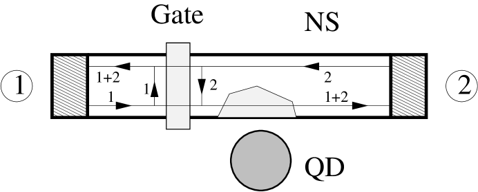
FIG. 2.: A two-terminal device. Scattering states emitted from the terminals are labeled by the terminals’ corresponding numbers. The interaction area is shown.

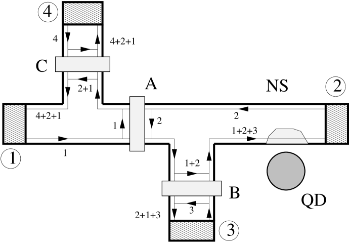
FIG. 3.: A four-terminal device. Scattering states emitted from the terminals are labeled by the terminals’ corresponding numbers. The interaction area is shown.

REFERENCES

- [1] R.M.Clark et al., Phys.Rev. B 52, 2656, 1995
- [2] J.P.Bird et al., Phys.Rev. B 51 , 18036, 1995; J.Phys.: Condens. Matter 10, L55,1998
- [3] U.Sivan, Y.Imry and A.Aronov, Europhys.Lett., 28,115, 1994
- [4] Ya.M.Blanter, cond-mat/9604101
- [5] A.Stern,Y.Aharonov and Y.Imry, Phys.Rev. 41, 3436, 1990
- [6] Y.Levinson, Europhys.Lett., 39,299, 1997
- [7] E.Buks et al. Physica 249-251, 295, 1998
- [8] I.L.Aleiner, N. S.Wingreen and Y.Meir, Phys.Rev.Lett. 79 , 3740, 1997
- [9] D.Sprinzak and M.Heiblum, unpublished
- [10] M.Buttiker and A.M.Martin, cond-mat/9902320
- [11] A.V.Uskov, K.Nishi and R.Lang, Appl.Phys.Lett. 74, 3081, 1999
- [12] B.L.Al’tshuler, A.G.Aronov and D.E.Khmelnitskii, J.Phys.C15, 7367, 1982
- [13] M.Field et al., Phys.Rev.Lett. 70 , 1311, 1993
- [14] M.Buttiker, Phys.Rev. B 46 , 12485, 1992
- [15] G.B.Lesovik, JETP Lett. 49, 592, 1989
- [16] L.Stodolsky, quant-ph/9805081
- [17] M.Buttiker, Phys.Rev. B 33 , 3020, 1986
- [18] E.V.Sukhorukov, unpublished
- [19] Y.B.Levinson and E.V.Sukhorukov, Phys.Lett. 149A, 167, 1990
- [20] Y.B.Levinson and E.V.Sukhorukov, J.Phys.: Condens.Matter 3, 7291, 1991