Contact resistance of quantum tubes

Abstract

We consider the conductance of a quantum tube connected to a metallic contact. The number of angular momentum states that the tube can support depends on the strength of the radial confinement. We calculate the transmission coefficients which yield the conductance via the Landauer formula, and discuss the relation of our results to armchair carbon nanotubes embedded in a metal. For Al and Au contacts and tubes with a realistic radial confinement we find that the transmission can be close to unity corresponding to a contact resistance close to $h/2e^{2}$ per band at the Fermi level in the carbon nanotube.

(Submitted )

1 Introduction

Since the recent discovery of the carbon nanotubes by Iijima [1] there has been a significant progress [2] in the studies of the conducting properties of both single-walled [3] and multi-walled [4] carbon nanotubes. Conductance of a mesoscopic system connected to metallic reservoirs is well understood and is usually described by the Landauer formula [5]. For quantum point contacts in semiconductor structures and in metallic nanowires it is well establish experimentally that the differential conductance to a good approximation is quantized in units of $G_{0}=2e^{2}/h$ and at zero temperature given by $G=G_{0}N$ where $N$ is the number of propagating modes. In carbon nanotubes with metallic contacts most experiments show that the conductance is less than the conductance which one should expect for a smooth interface between tube and metal, e.g. $G=4e^{2}/h$ for metallic single-walled tubes where the extra factor of 2 comes from the two $\pi$ bands that are crossing the Fermi level [6]. The reasons for this lower conductance are still not fully known. Theoretically, several groups have considered the effects of vacancies [7], disorder [8], distortion [9], and doping [10] on the conductance of carbon nanotubes. The conducting properties have also been studied in e.g. the context of junctions between different metallic carbon nanotubes [11], Aharonow–Bohm effect in the presence of a magnetic field [12], and the Luttinger liquid behavior of a one-dimensional gas of interacting electrons [13]. Also the ideal “hollow quantum cylinder”, i.e. a two-dimensional electron gas on a cylinder, has been studied in context of the difference between strip-like wires and tubes [14]. However, with the exception of the recent qualitative study of Tersoff [15] and the recent modeling-works of Anantram et al. [16] and Sanvito et al. [17], less attention has been focused on the conditions for a good transmission between tube and a metal contact which is an important issue for practical devices with carbon nanotubes, or other quantum tubes.

In quantum point contacts an adiabatic interface between the wire and reservoirs ensures a transmission coefficient close to unity [18]. The condition for adiabaticity is that the shape of the contact region varies slowly on the scale of the Fermi wave length. In the opposite case with an abrupt interface, i.e. quasi-one-dimensional lead connected to a wide two-dimensional contact, Szafer and Stone [19] found that the transmission rapidly increases to unity as the width of the confined region exceeds half of the Fermi wavelength, thus giving a reflectionless contact.

For the contact between a quantum tube and a three-dimensional metal it is not obvious that the assumption of an ideal reflectionless contact applies and the aim of this work is to study the contact resistance for this case.

The model we are studying is that of a hollow quantum cylinder of radius $R_{\scriptscriptstyle\rm T}$ contacted by a three-dimensional free-electron metal which we for convenience model by a cylindrical wire with radius $R_{\scriptscriptstyle\rm C}\gg R_{\scriptscriptstyle\rm T}$, see Fig. 1. The system thus has full cylindrical symmetry and the angular momentum quantum number $m$ can therefore be used to label the scattering states.

For the coupling of the quantum tube to the contact it is necessary to take a radial confinement potential for the quantum tube into account and here we model the confinement by an attractive delta-function potential. As an example we apply this model to metal contacts of Al or Au; the quantum tube parameters are chosen to mimic armchair carbon nanotubes: the strength of the confinement can be related to the work function for the material that constitutes the tube and in the case of a carbon nanotube we relate it to the work function of graphene. It should be noted that the employed free electron model does not fully describe the actual band structure of carbon nanotubes. Nevertheless, a study of contact resistance within this idealized model should yield valuable insights which are relevant to real materials.

The paper is organized as follows: In Section II the eigenstates of a quantum tube connected to a cylindrical metal contact are found. In Section III these eigenstates are used to construct the scattering states to find the transmission coefficient, and hence the conductance of the contact. In Section IV, we apply our model to contacts between an armchair carbon nanotube and a metal. Finally, in Section V discussion and conclusions are given. Essential details of analytical calculations are given in Appendices A and B.

2 The eigenstates

We separate the discussion into two parts: first we find the eigenstates in the tubular geometry and then the eigenstates for the cylindrical metal contact. In Section III the matching of these eigenstates are used to construct the scattering states of the contact.

2.1 Quantum tube

The quantum tube of radius $R_{\scriptscriptstyle\rm T}$ with otherwise free electrons is modeled by the Hamiltonian

$$\hat{{\cal{H}}}_{\scriptscriptstyle\rm T}=-\frac{\hbar^{2}}{2m_{e}}\left[\frac{\partial^{2}}{\partial z^{2}}+\frac{\partial^{2}}{\partial r^{2}}+\frac{1}{r}\frac{\partial}{\partial r}+\frac{1}{r^{2}}\frac{\partial^{2}}{\partial\phi^{2}}\right]+V_{\scriptscriptstyle\rm T}(r),$$ (1)

with a confining potential given by an attractive delta function potential

$$V_{\scriptscriptstyle\rm T}(r)=-H\delta(r-R_{\scriptscriptstyle\rm T}),$$ (2)

where the confinement strength $H$ is taken positive.

The eigenstates of the Schrödinger equation have the form

$$\Psi_{m}(r,\phi,z)=R_{m}(r)\chi_{m}(\phi)\psi_{m}(z),$$ (3)

with angular and longitudinal wave functions

$$\chi_{m}(\phi) = (2\pi)^{-1/2}\exp[im\phi],$$ (4)

$$\psi_{m}(z) = \left[k_{m}(E)\right]^{-1/2}\exp\left[\pm ik_{m}(E)z\right],$$ (5)

where the angular momentum quantum numbers $m$ are integers, $k_{m}(E)=\left[\frac{2m_{e}}{\hbar^{2}}\left(E-\varepsilon_{m}\right)\right]^{1/2}$ is the wave vector associated to the longitudinal free propagation, and $E=E_{m}+\varepsilon_{m}$ is the total energy of the state. Here, $E_{m}>0$ is the energy associated to the longitudinal propagation and $\varepsilon_{m}<0$ is the (binding) energy associated to the transverse motion. We can relate the strength of the confinement to the work function $W=\left|\varepsilon_{m}\right|-\hbar^{2}k_{{\rm F}}^{2}/2m_{e}$, which is the energy required to remove an electron at the Fermi level (disregarding surface charge effects). The normalization $\left[k_{m}(E)\right]^{-1/2}$ is chosen such that the propagating modes carry the same amount of current.

The radial wave function $R_{m}(r)$ satisfies

$$\left\{r^{2}\frac{\partial^{2}}{\partial r^{2}}+r\frac{\partial}{\partial r}+\left[\frac{2m_{e}\varepsilon_{m}}{\hbar^{2}}r^{2}-m^{2}\right]\right\}R_{m}(r)=-\gamma R_{\scriptscriptstyle\rm T}\delta(r-R_{\scriptscriptstyle\rm T})R_{m}(r),$$ (6)

where $\gamma\equiv 2m_{e}HR_{\scriptscriptstyle\rm T}/\hbar^{2}$ is a dimensionless confinement strength. For the bound states ($\varepsilon_{m}<0$) and $r\neq R_{\scriptscriptstyle\rm T}$ this equation has the form of Bessel’s modified differential equation [20]. The solutions are given by modified Bessel functions of order $m$ of the first and second kind, so that the full solution is given by

$$R_{m}(r) = \left\{\begin{array}[]{ccc}A_{m}I_{m}(\kappa_{m}r)&,&r<R_{\scriptscriptstyle\rm T}\\ B_{m}K_{m}(\kappa_{m}r)&,&r>R_{\scriptscriptstyle\rm T}\end{array}\right.,$$ (9)

where $\kappa_{m}\equiv\left[2m_{e}\left|\varepsilon_{m}\right|/\hbar^{2}\right]^{1/2}$. At $r=R_{\scriptscriptstyle\rm T}$, the radial wave function is continuous and the appropriate matching condition for the derivative $\partial R_{m}(r)/\partial r$ at $r=R_{\scriptscriptstyle\rm T}$ is found by integrating Eq. (6) from $R_{\scriptscriptstyle\rm T}^{-}=R_{\scriptscriptstyle\rm T}-0^{+}$ to $R_{\scriptscriptstyle\rm T}^{+}=R_{\scriptscriptstyle\rm T}+0^{+}$. In this way the matching conditions become

$$R_{m}(R_{\scriptscriptstyle\rm T}^{+})-R_{m}(R_{\scriptscriptstyle\rm T}^{-}) = 0,$$ (10)

$$\left.\frac{\partial R_{m}(r)}{\partial r}\right|_{R_{\scriptscriptstyle\rm T}^{+}}-\left.\frac{\partial R_{m}(r)}{\partial r}\right|_{R_{\scriptscriptstyle\rm T}^{-}} = -\gamma\frac{R_{m}(R_{\scriptscriptstyle\rm T})}{R_{\scriptscriptstyle\rm T}},$$ (11)

and we get the following equation for the normalization coefficients

$$\left(\begin{array}[]{cc}I_{m}(\kappa_{m}R_{\scriptscriptstyle\rm T})&-K_{m}(\kappa_{m}R_{\scriptscriptstyle\rm T})\\ I_{m-1}(\kappa_{m}R_{\scriptscriptstyle\rm T})+I_{m+1}(\kappa_{m}R_{\scriptscriptstyle\rm T})-\frac{2\gamma I_{m}(\kappa_{m}R_{\scriptscriptstyle\rm T})}{\kappa_{m}R_{\scriptscriptstyle\rm T}}&K_{m-1}(\kappa_{m}R_{\scriptscriptstyle\rm T})+K_{m+1}(\kappa_{m}R_{\scriptscriptstyle\rm T})\end{array}\right)\left(\begin{array}[]{c}A_{m}\\ B_{m}\end{array}\right)=\left(\begin{array}[]{c}0\\ 0\end{array}\right).$$ (12)

Non-trivial solutions exist if the determinant vanishes, and hereby the wave vector $\kappa_{m}$ is a solution to the equation

$$\gamma^{-1}=I_{m}(\kappa_{m}R_{\scriptscriptstyle\rm T})K_{m}(\kappa_{m}R_{\scriptscriptstyle\rm T}),$$ (13)

where the result for the Wronskian $W\left\{K_{m}\left(x\right);I_{m}\left(x\right)\right\}=1/x$ has been used [20]. Expanding Eq. (13) in the small-$\kappa_{m}R_{\scriptscriptstyle\rm T}$ limit [20] we find that a bound state with angular momentum $m\hbar$ exists for $\gamma>2m$. The number of bound states for a certain value of $\gamma$ is given by $N={\rm Int}(\gamma/2)+1$ where ${\rm Int}(x)$ is the integer part of $x$. Thus, there is always at least a single bound state corresponding to $m=0$.

From the matching conditions and the normalization of $R_{m}$ (see Appendix A), it follows that

$$R_{m}(r) = A_{m}\times\left\{\begin{array}[]{ccc}I_{m}(\kappa_{m}r)&,&r<R_{\scriptscriptstyle\rm T}\\ \frac{I_{m}(\kappa_{m}R_{\scriptscriptstyle\rm T})}{K_{m}(\kappa_{m}R_{\scriptscriptstyle\rm T})}K_{m}(\kappa_{m}r)&,&R_{\scriptscriptstyle\rm T}<r\end{array}\right.,$$ (16)

$$A_{m} = \frac{\sqrt{2}}{R_{\scriptscriptstyle\rm T}}\left[\frac{I_{m}^{2}(\kappa_{m}R_{\scriptscriptstyle\rm T})}{K_{m}^{2}(\kappa_{m}R_{\scriptscriptstyle\rm T})}K_{m-1}(\kappa_{m}R_{\scriptscriptstyle\rm T})K_{m+1}(\kappa_{m}R_{\scriptscriptstyle\rm T})-I_{m-1}(\kappa_{m}R_{\scriptscriptstyle\rm T})I_{m+1}(\kappa_{m}R_{\scriptscriptstyle\rm T})\right]^{-1/2}.$$ (17)

A plot of the radial wave function is shown in the inset of Fig. 3. Increasing the confinement strength, the radial wave function becomes more localized which is accompanied by an increase in the binding energy.

2.2 Metal contacts

For the metal it is convenient to assume a cylindrical geometry and consider a cylindrical wire of radius $R_{\scriptscriptstyle\rm C}\gg R_{\scriptscriptstyle\rm T}$. The Hamiltonian is written as

$$\hat{{\cal{H}}}_{\scriptscriptstyle\rm C}=-\frac{\hbar^{2}}{2m_{e}}\left[\frac{\partial^{2}}{\partial z^{2}}+\frac{\partial^{2}}{\partial r^{2}}+\frac{1}{r}\frac{\partial}{\partial r}+\frac{1}{r^{2}}\frac{\partial^{2}}{\partial\phi^{2}}\right]+V_{\scriptscriptstyle\rm C}(r),$$ (18)

with a hard-wall confining potential

$$V_{\scriptscriptstyle\rm C}(r)=\left\{\begin{array}[]{ccc}-V_{\scriptscriptstyle\rm C}^{0}&,&r<R_{\scriptscriptstyle\rm C}\\ \infty&,&R_{\scriptscriptstyle\rm C}<r\end{array}\right..$$ (19)

Obviously, for $r\geq R_{\scriptscriptstyle\rm C}$, $\Psi(r,\phi,z)=0$ and for $r<R_{\scriptscriptstyle\rm C}$ the eigenstates have the form

$$\Psi_{\nu m}(r,\phi,z) = R_{\nu m}(r)\chi_{m}(\phi)\psi_{\nu m}(z),$$ (20)

$$R_{\nu m}(r) = C_{\nu m}J_{m}(\kappa_{\nu m}r),$$ (21)

$$\chi_{m}(\phi) = (2\pi)^{-1/2}\exp[im\phi],$$ (22)

$$\psi_{\nu m}(z) = \left[k_{\nu m}(E)\right]^{-1/2}\exp\left[\pm ik_{\nu m}(E)z\right],$$ (23)

where $J_{m}$ is a Bessel function of the first kind of order $m$, $\kappa_{\nu m}^{2}=2m_{e}\varepsilon_{\nu m}/\hbar^{2}$ is a wave vector corresponding to the radial energy $\varepsilon_{\nu m}$, $k_{\nu m}(E)=\left[\frac{2m_{e}}{\hbar^{2}}\left(E+V_{\scriptscriptstyle\rm C}^{0}-\varepsilon_{\nu m}\right)\right]^{1/2}$ is the wave vector of the longitudinal motion, and $E$ is the total energy of the state. Again the normalization $\left[k_{\nu m}(E)\right]^{-1/2}$ makes the propagating modes carry the same amount of current.

The boundary condition for the radial wave function leads to $J_{m}(\kappa_{\nu m}R_{\scriptscriptstyle\rm C})=0,$ from which we find $\kappa_{\nu m}$ numerically. Since $J_{m}(x)\sim(2/\pi x)^{1/2}\cos(x-m\pi/2-\pi/4)$ for large $x$ [20], we have $\kappa_{\nu m}R_{\scriptscriptstyle\rm C}\simeq(\nu+m/2-1/4)\pi$ with $\nu=1,2,3,\ldots$. The normalization $C_{\nu m}$ is given by (see Appendix A)

$$C_{\nu m}=\frac{1}{R_{\scriptscriptstyle\rm C}}\sqrt{\frac{2}{-J_{m-1}(\kappa_{\nu m}R_{\scriptscriptstyle\rm C})J_{m+1}(\kappa_{\nu m}R_{\scriptscriptstyle\rm C})}},$$ (24)

which is a real number.

3 Transmission of contact

We consider an electron in the tube in mode $m$ incident on the contact (see Fig. 1) and compute the transmission and reflection coefficients. We construct the scattering states in the basis of the eigenstates of the Schrödinger equation (see previous section). Since the angular momentum is a conserved quantity, the transmitted and reflected parts of the wave function also have the same quantum number $m$. In the quantum tube ($z<0$) the scattering state is given by

$$\Psi_{m}(r,\phi,z)=R_{m}(r)\frac{\exp(im\phi)}{\sqrt{2\pi}}\left[\frac{\exp(ik_{m}z)}{\sqrt{k_{m}}}+r_{m}\frac{\exp(-ik_{m}z)}{\sqrt{k_{m}}}\right],$$ (25)

and in the contact ($z>0$) by

$$\Psi_{m}(r,\phi,z)=\sum_{\nu=1}^{\infty}t_{\nu m}R_{\nu m}(r)\frac{\exp(im\phi)}{\sqrt{2\pi}}\frac{\exp(ik_{\nu m}z)}{\sqrt{k_{\nu m}}}.$$

Here $r_{m}$ is the reflection amplitude for mode $m$ and $t_{\nu m}$ is the corresponding transmission amplitude. We assume that the effective electron mass is the same in the two materials so that the continuity of $\Psi_{m}(r,\phi,z)$ and $\partial\Psi_{m}(r,\phi,z)/\partial z$ at $z=0$ are appropriate boundary conditions. For carbon nanotubes and metals like Al and Au this is a reasonable approximation ($m_{e}^{\star}\sim 1.2\,m_{0}$ [21]). For general details on how to account for differences in the effective mass and the underlying symmetry of the lattice we refer to Refs. [22] and references therein. The boundary conditions lead to

$$r_{m} = \frac{1-\sum_{\nu=1}^{\infty}\varrho_{\nu m}^{2}}{1+\sum_{\nu=1}^{\infty}\varrho_{\nu m}^{2}},$$ (26)

$$t_{\nu m} = \frac{2\varrho_{\nu m}}{1+\sum_{\nu=1}^{\infty}\varrho_{\nu m}^{2}},$$ (27)

where $\varrho_{\nu m}\equiv\sqrt{k_{\nu m}/k_{m}}\left\langle R_{m}\left|R_{\nu m}\right.\right\rangle$, with the radial overlap defined as $\left\langle R_{m}\left|R_{\nu m}\right.\right\rangle\equiv\int_{0}^{\infty}{\rm d}r\,rR_{m}(r)R_{\nu m}(r).$ In addition we have the sum-rule $\sum_{\nu=1}^{\infty}\left\langle R_{m}\left|R_{\nu m}\right.\right\rangle^{2}=1$, which can be used to verify the numerical convergence. The overlap can be calculated analytically (see Appendix B) and the squared overlap is given by

$$\left<R_{m}\left|R_{\nu m}\right.\right>^{2} = \left(\frac{R_{\scriptscriptstyle\rm T}}{R_{\scriptscriptstyle\rm C}}\right)^{2}\frac{\left[J_{m}(\kappa_{\nu m}R_{\scriptscriptstyle\rm T})+\kappa_{\nu m}I_{m}(\kappa_{m}R_{\scriptscriptstyle\rm T})K_{m}(\kappa_{m}R_{\scriptscriptstyle\rm C})J_{m+1}(\kappa_{\nu m}R_{\scriptscriptstyle\rm C})\right]^{2}}{\left[\left(\kappa_{m}R_{\scriptscriptstyle\rm T}\right)^{2}+\left(\kappa_{\nu m}R_{\scriptscriptstyle\rm T}\right)^{2}\right]^{2}\left[J_{m-1}(\kappa_{\nu m}R_{\scriptscriptstyle\rm C})J_{m+1}(\kappa_{\nu m}R_{\scriptscriptstyle\rm C})\right]}$$

$$\times\frac{4}{\left[K_{m}^{2}(\kappa_{m}R_{\scriptscriptstyle\rm T})I_{m-1}(\kappa_{m}R_{\scriptscriptstyle\rm T})I_{m+1}(\kappa_{m}R_{\scriptscriptstyle\rm T})-I_{m}^{2}(\kappa_{m}R_{\scriptscriptstyle\rm T})K_{m-1}(\kappa_{m}R_{\scriptscriptstyle\rm T})K_{m+1}(\kappa_{m}R_{\scriptscriptstyle\rm T})\right]}.$$

The total transmission from mode $m$ in the quantum tube into the contact is thus

$${\cal T}_{m} = \sum_{\nu=1}^{\infty}{\cal{P}}_{\nu m}\left|t_{\nu m}\right|^{2}$$ (29)

$$= \left|\frac{2}{1+\sum_{\nu=1}^{\infty}\varrho_{\nu m}^{2}}\right|^{2}\sum_{\nu=1}^{\infty}{\cal{P}}_{\nu m}\varrho_{\nu m}^{2},$$

where ${\cal{P}}_{\nu m}$ projects onto the propagating modes ($k_{\nu m}$ real) of the metal contact. Here we have assumed that the lengths of the quantum tube and the contact are semi-infinite so that tunneling through evanescent modes can be neglected. These should be included in the case of two metal contacts connected by a quantum tube of finite length. Introducing real and imaginary parts by $\sum_{\nu=1}^{\infty}\varrho_{\nu m}^{2}\equiv{\Gamma}_{m}^{\prime}+i{\Gamma}_{m}^{\prime\prime}$ we obtain

$${\cal T}_{m}=\frac{4{\Gamma}_{m}^{\prime}}{\left(1+{\Gamma}_{m}^{\prime}\right)^{2}+{{\Gamma}_{m}^{\prime\prime}}^{2}}.$$ (30)

The reflection probability ${\cal R}_{m}$ can be calculated in a similar manner which provides us with the usual sum-rule ${\cal T}_{m}+{\cal R}_{m}=1$, ensuring the conservation of probability current density.

To summarize, the transmission probability of mode $m$ can be calculated from Eq. (30) with $k_{m}(E)=\left[\frac{2m_{e}}{\hbar^{2}}\left(E-\varepsilon_{m}\right)\right]^{1/2}$ and $k_{\nu m}(E)=\left[\frac{2m_{e}}{\hbar^{2}}\left(E+V_{\scriptscriptstyle\rm C}^{0}-\varepsilon_{\nu m}\right)\right]^{1/2}$, with $\varepsilon_{m}=\frac{\hbar^{2}}{2m_{e}}\kappa_{m}^{2}$ being the energy of the $m$th transverse mode in the tube and similarly $\varepsilon_{\nu m}=\frac{\hbar^{2}}{2m_{e}}\kappa_{\nu m}^{2}$ is the transverse energy in the contact. Here $\kappa_{m}$ and $\kappa_{\nu m}$ are solutions to $I_{m}(\kappa_{m}R_{\scriptscriptstyle\rm T})K_{m}(\kappa_{m}R_{\scriptscriptstyle\rm T})=\gamma^{-1}$ and $J_{m}(\kappa_{\nu m}R_{\scriptscriptstyle\rm C})=0$, respectively. For a numerical implementation, an upper cut-off $\nu_{c}$ in the sum over modes in the contact is needed and the sum-rule for the squared radial overlap is then a measure of the numerical convergence for a given cut-off.

When choosing values for the confinement parameters, $\gamma$ and $V_{\scriptscriptstyle\rm C}^{0}$, we take into account that the Fermi momenta of the quantum tube and the metal can be different since the relevant electrons are located at the Fermi levels of the two materials. For the metal contact we use the known Fermi energies for e.g. Al and Au to relate the confinement potential to the Fermi level as $E_{\rm F}^{\scriptscriptstyle\rm C}=E+V_{\scriptscriptstyle\rm C}^{0}$, with the Fermi energy being defined positive. For the tube, the Fermi energy enters as $E_{{\rm F}}^{\scriptscriptstyle\rm T}=E+|\varepsilon_{m}|$. When the two materials are brought into contact the chemical potentials align, but the difference in Fermi wave vectors remains. Thus for the metal contact $E+V_{\scriptscriptstyle\rm C}^{0}=\hbar^{2}\left[k_{{\rm F}}^{\scriptscriptstyle\rm C}\right]^{2}/2m_{e}$, and for the tube $E+|\varepsilon_{m}|=\hbar^{2}\left[k_{{\rm F}}^{\scriptscriptstyle\rm T}\right]^{2}/2m_{e}$. For the tube we need to specify $\gamma$, which follows from the work function $W=|\varepsilon_{m}|-\hbar^{2}\left[k_{{\rm F}}^{\scriptscriptstyle\rm T}\right]^{2}/2m_{e}$. We have neglected the charge density induced at the interface by a mismatch of the work functions. For a discussion of this in the context of the screening properties of one-dimensional systems, see e.g. Ref. [23].

4 Contact resistance of single-walled armchair carbon nanotubes

The $(n,n)$ armchair single-walled carbon nanotube can be regarded as the result of rolling one sheet of graphite (with the carbon atoms in a hexagonal lattice) in the direction of one of the bonds [21]. The resulting tube has a periodicity $a\simeq 0.246\,{\rm nm}$ along the tube axis ($z$-axis) and a radius $R_{\scriptscriptstyle\rm T}\simeq n\times\sqrt{3}a/2\pi$ with $4n$ atoms along the perimeter, arranged in two rows that resemble a chain of armchairs, see Fig. 2. Their metallic character is caused by two $\pi$ bands crossing the Fermi level at a wave vector $k_{{\rm F}}^{\scriptscriptstyle\rm T}\simeq 2\pi/3a$.

As discussed recently by Tersoff [15] the metallic armchair carbon nanotubes have electrons at the Fermi level which can be regarded as having an angular momentum quantum number $m=0$. In order to apply our simple model to the problem of the contact resistance of $(n,n)$ single-walled carbon nanotubes embedded in a free-electron metal we notice that $k_{{\rm F}}^{\scriptscriptstyle\rm T}R_{\scriptscriptstyle\rm T}\simeq n/\sqrt{3}$. In Fig. 3 the transmission probability at the Fermi level is shown for several values of $k_{\rm F}^{\scriptscriptstyle\rm T}R_{\scriptscriptstyle\rm T}$ corresponding to $(n,n)$ armchair carbon nanotubes for various values of the dimensionless confinement strength $\gamma$. In the particular case of an Al contact, the mismatch is given by $k_{{\rm F}}^{\scriptscriptstyle\rm T}/k_{{\rm F}}^{\scriptscriptstyle{\rm Al}}\sim 0.49$ and the corresponding transmission is presented in panel (a) of Fig. 4. In panel (b) we show similar results for an Au contact for which $k_{{\rm F}}^{\scriptscriptstyle\rm T}/k_{{\rm F}}^{\scriptscriptstyle{\rm Au}}\sim 0.70$.

In order to estimate $\gamma$ we relate it to the work function of the carbon nanotube which is of the order $4-5\,{\rm eV}$. For the quantum tube we associate a work function to the $m=0$ bound state via its binding energy, i.e. $W\equiv\frac{\hbar^{2}\kappa_{0}^{2}}{2m_{e}}-E_{{\rm F}}^{\scriptscriptstyle\rm T}$ where $\kappa_{0}$ is the solution to $I_{0}(\kappa_{0}R_{\scriptscriptstyle\rm T})K_{0}(\kappa_{0}R_{\scriptscriptstyle\rm T})=\gamma^{-1}$. In Fig. 5 this work function is shown as a function of the confinement strength for quantum tubes corresponding to $(n,n)$ armchair carbon nanotubes. From this we estimate that $\gamma<10-20$ is a reasonable regime for the curves shown in Figs. 3 and 4. This means that a transmission close to unity (per band at the Fermi level) can be expected if the armchair nanotube is embedded in free-electron metals like Al or Au. Assuming a work function $W=4.5\,{\rm eV}$ of the nanotube we have used the corresponding value of $\gamma$ to calculate the transmission for the different nanotubes. For $(n,n)$ armchair nanotubes with Al and Au contacts we find ${\cal T}_{\scriptscriptstyle\rm Al}\sim 0.93$ and ${\cal T}_{\scriptscriptstyle\rm Au}\sim 0.98$, respectively. In the case of matching Fermi wave vectors ($k_{{\rm F}}^{\scriptscriptstyle{\rm T}}/k_{{\rm F}}^{\scriptscriptstyle{\rm C}}=1$) we get ${\cal T}\sim 0.87$. For the considered tubes ($3\leq n\leq 17$), these transmissions are found to be almost independent of the specific value of the tube indices $(n,n)$.

Here we have only taken the geometry-related contact scattering into account. Physically, a lower transmission can be caused by electrons being scattered by interface imperfections/roughness, deviations from a spherical Fermi surface of the metal contact, and scattering due to non-matching work functions of the nanotube and metal. Also scattering due to the non-matching Fermi velocities of the nanotube and the metal could be expected. However, as shown in Fig. 4, a mismatch between Fermi wave vectors can actually in some cases increase the transmission (and thereby the conductance) due to quantum interferences, even though the mismatch by itself is known to give rise to momentum relaxation and thereby resistance.

5 Discussion and conclusion

We have considered the contact resistance (in terms of transmission) of a quantum tube embedded in a free-electron metal. For the quantum tube we have modeled the radial confinement of the electron motion by an attractive delta function potential which gives rise to at least one bound state in the radial direction. The strength of the attractive potential can phenomenologically be associated to the work function of the quantum tube. Within this model we have calculated the transmission of a quantum tube contacted by a free-electron metal. Due to the cylindrical geometry of the contact, considerable analytical progress was possible and with the resulting equations the scattering problem is readily solved numerically.

As an application we have considered the transparency of contacts with armchair carbon nanotubes embedded in free-electron metals. Our calculations show that in the absence of scattering mechanisms associated to e.g. interface imperfections/roughness, deviations from a spherical Fermi surface of the metal contact, and scattering due to non-matching work functions of the nanotube and metal, the geometry itself allows for a high transparent contact between armchair carbon nanotubes and free-electron metal contacts. Furthermore, from this simple model we find that Al would be a good candidate for such a metal as it was suggested recently by Tersoff [15]. For Au however, we find that the present 3D geometry allows for good contact in contrast to Tersoff’s findings for Au, which were based on 1D considerations.

A Normalization of radial wave functions

From the radial wave function of the quantum tube, Eq. (16), it follows that the normalization is given by

$$A_{m}=\kappa_{m}\left[\int_{0}^{\kappa_{m}R_{\scriptscriptstyle\rm T}}{\rm d}\alpha\,\alpha I_{m}^{2}(\alpha)+\frac{I_{m}^{2}(\kappa_{m}R_{\scriptscriptstyle\rm T})}{K_{m}^{2}(\kappa_{m}R_{\scriptscriptstyle\rm T})}\int_{\kappa_{m}R_{\scriptscriptstyle\rm T}}^{\infty}{\rm d}\alpha\,\alpha K_{m}^{2}(\alpha)\right]^{-1/2},$$ (31)

and since [24]

$$\int{\rm d}\alpha\,\alpha I_{m}^{2}(\alpha) = {\alpha}^{2}\left[I_{m}^{2}({\alpha})-I_{m-1}({\alpha})I_{m+1}({\alpha})\right]/2,$$ (32)

$$\int{\rm d}\alpha\,\alpha K_{m}^{2}(\alpha) = {\alpha}^{2}\left[K_{m}^{2}({\alpha})-K_{m-1}({\alpha})K_{m+1}({\alpha})\right]/2,$$ (33)

we get the result in Eq. (17). Similarly, from the radial wave function of the free-electron metal contact, Eq. (21), it follows that the normalization is given by

$$C_{\nu m}=\left[\int_{0}^{R_{\scriptscriptstyle\rm C}}{\rm d}r\,rJ_{m}^{2}(\kappa_{\nu m}r)\right]^{-1/2},$$ (34)

and since $J_{m}(\kappa_{\nu m}R_{\scriptscriptstyle\rm C})=0$ and [24]

$$\int{\rm d}\alpha\,\alpha J_{m}^{2}(\alpha)=\alpha^{2}\left[J_{m}^{2}(\alpha)-J_{m-1}(\alpha)J_{m+1}(\alpha)\right]/2,$$ (35)

we obtain Eq. (24).

B Overlap of radial wave functions

The overlap of radial wave functions can be written as

$$\left<R_{m}\left|R_{\nu m}\right.\right> = A_{m}C_{\nu m}\left[\int_{0}^{R_{\scriptscriptstyle\rm T}}{\rm d}r\,rI_{m}(\kappa_{m}r)J_{m}(\kappa_{\nu m}r)+\frac{I_{m}(\kappa_{m}R_{\scriptscriptstyle\rm T})}{K_{m}(\kappa_{m}R_{\scriptscriptstyle\rm T})}\int_{R_{\scriptscriptstyle\rm T}}^{R_{\scriptscriptstyle\rm C}}{\rm d}r\,rK_{m}(\kappa_{m}r)J_{m}(\kappa_{\nu m}r)\right]$$ (36)

$$= \frac{A_{m}C_{\nu m}}{\kappa_{m}^{2}+\kappa_{\nu m}^{2}}\frac{J_{m}(\kappa_{\nu m}R_{\scriptscriptstyle\rm T})+\kappa_{\nu m}R_{\scriptscriptstyle\rm C}I_{m}(\kappa_{m}R_{\scriptscriptstyle\rm T})K_{m}(\kappa_{m}R_{\scriptscriptstyle\rm C})J_{m+1}(\kappa_{\nu m}R_{\scriptscriptstyle\rm C})}{K_{m}(\kappa_{m}R_{\scriptscriptstyle\rm T})},$$

where we have used the integrals [24]

$$\int{\rm d}r\,rI_{m}(\alpha r)J_{m}(\beta r) = \frac{r\left\{\alpha I_{m+1}(\alpha r)J_{m}(\beta r)+\beta I_{m}(\alpha r)J_{m+1}(\beta r)\right\}}{\alpha^{2}+\beta^{2}},$$ (37)

$$\int{\rm d}r\,rK_{m}(\alpha r)J_{m}(\beta r) = -\frac{r\left\{\alpha K_{m+1}(\alpha r)J_{m}(\beta r)-\beta K_{m}(\alpha r)J_{m+1}(\beta r)\right\}}{\alpha^{2}+\beta^{2}},$$ (38)

together with the boundary condition $R_{\nu m}(R_{\scriptscriptstyle\rm C})=0$.

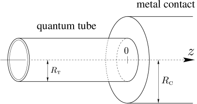
Fig.  1: Contact between a quantum tube ($z<0$) of radius $R_{\scriptscriptstyle\rm T}$ and a three-dimensional cylindrical free-electron metallic wire ($z>0$) of radius $R_{\scriptscriptstyle\rm C}\gg R_{\scriptscriptstyle\rm T}$.

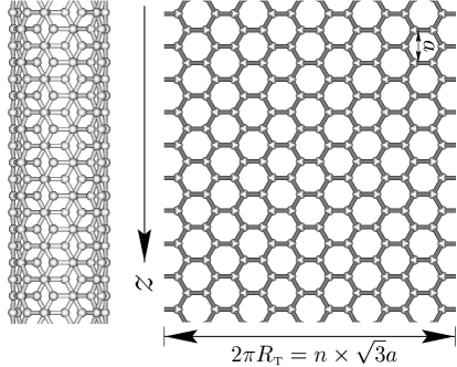
Fig.  2: A sheet of graphite (upper panel) which can be rolled up to a $(n,n)$ armchair single-walled carbon nanotube (lower panel). The tube has a periodicity $a\simeq 0.246\,{\rm nm}$ along the tube axis ($z$-axis) and a radius $R_{\scriptscriptstyle\rm T}\simeq n\times\sqrt{3}a/2\pi$ with $4n$ carbon atoms along the perimeter, arranged in two rows that resemble a chain of armchairs. The shown example is a $(5,5)$ armchair nanotube.

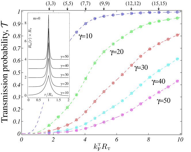
Fig.  3: Transmission probability ${\cal T}$ from an $(n,n)$ armchair carbon nanotube of radius $R_{\scriptscriptstyle\rm T}\simeq n/\sqrt{3}k_{{\rm F}}$ into a cylindrical contact with radius $R_{\scriptscriptstyle\rm C}\gg R_{\scriptscriptstyle\rm T}$. ${\cal T}$ is shown for several values of the confinement strength $\gamma$. The results marked with $\otimes$ are the specific values of $R_{\scriptscriptstyle\rm T}k_{{\rm F}}=n/\sqrt{3}$ corresponding to $(n,n)$ tubes and the dashed lines are calculated curves which are shown as guides to the eye. The inset shows the radial wave function of the quantum tube, Eq. (16), for $m=0$. The nanotube and the metal are assumed to have the same Fermi wave vectors, so that $k_{{\rm F}}^{\scriptscriptstyle{\rm T}}/k_{{\rm F}}^{\scriptscriptstyle{\rm C}}=1$.

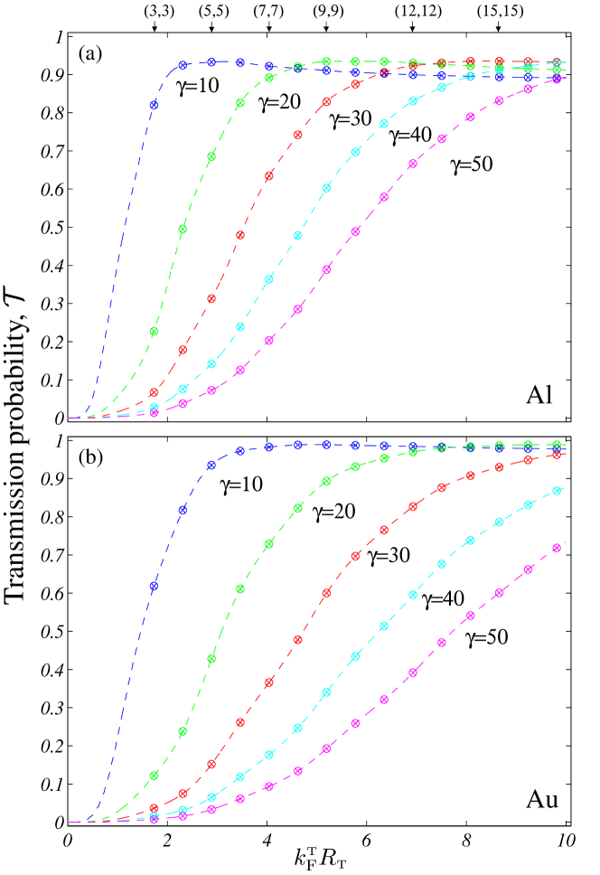
Fig.  4: The same calculation as in Fig. 3, but, with a mismatch between the Fermi wave vectors of the carbon nanotube and the metal. Panel (a) is for $k_{{\rm F}}^{\scriptscriptstyle{\rm T}}/k_{{\rm F}}^{\scriptscriptstyle{\rm Al}}\sim 0.49$ corresponding to nanotubes embedded in an Al contact and panel (b) is for $k_{{\rm F}}^{\scriptscriptstyle{\rm T}}/k_{{\rm F}}^{\scriptscriptstyle{\rm Au}}\sim 0.70$ corresponding to nanotubes embedded in an Au contact.

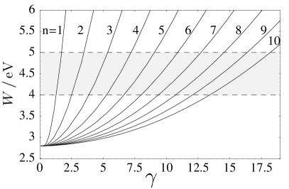
Fig.  5: Work function $W$ of quantum tubes corresponding to $(n,n)$ armchair carbon nanotube as a function of the dimensionless confinement strength $\gamma$. Experimentally, the work function of a carbon nanotube is $W\sim 4-5\,{\rm eV}$ which for the shown nanotubes means that $\gamma<10-20$ is the important parameter range.