WISC-TH-99-353

GENERALIZED RANDOM PHASE APPROXIMATION:
Zero and Non-Zero Temperature Properties of an Interacting Electron Gas

A. REBEI

Department of Physics
University of Wisconsin-Madison
Madison, WI 53706

W.N.G. HITCHON
Materials Science Program
University of Wisconsin-Madison
Madison, WI 53706

Correlated systems at both zero and nonzero temperature are treated here from a novel angle using a functional method. This functional method is an extension of the usual effective potential method. Here, however the effective action is made to depend explicitly on the correlation effects that are inherent in the physics involved. This will enable us to obtain new expressions for the free energy, the specific heat and the ground state energy. The new expansion is shown to give the expected results for the homogeneous case at zero temperature. However at non-zero temperature we are able to get new sets of diagrams that have a vanishing effect at zero temperature. To lowest order these diagrams if summed properly will solve a $\ln T$ anomaly in the specific heat of an electron gas at low temperature. We are also able to show that this method provides a very clear way to extend the RPA approximation. We calculate the effect of exchange on the ring diagrams at zero temperature and show how to include some of the ladder diagrams. Our results agree well with known numerical calculations. We conclude by showing that this method is in fact a variant of the time dependent density functional method and can in principle be applied to study the effects of correlation in the nonhomogeneous case.

PACS :71.10.Ca, 05.30.-d, 05.30.Fk, 31.15.Gy, 71.27.+a, 71.15.Mb

1 Introduction

Strongly correlated systems continue to be a popular subject due to the importance of these systems in physical processes in general. Electron systems form an important subset of these systems. The nonlinearity that appears in this type of problem complicates greatly the calculation of any physical properties of the system that strongly depend on the correlation between the individual particles. In this paper we are mainly concerned with a particular aspect of this area, that is, of calculating the ground state equilibrium energy of a large Fermi gas in an external potential, at both zero and at nonzero temperature. At zero temperature the random phase approximation (RPA) is a well known method which addresses this problem. Here we present a way to improve on it, using an effective action method, which includes higher order interactions in a consistent way. This new method is also applicable at finite temperature. At low temperature, the  new method shows clearly the importance of the so called “anomalous diagrams” in cancelling the non-physical $\ln T$ term in the specific heat [1]. Another important aspect of this new approach is that it is applicable to nonhomogeneous Fermi systems. The currently popular method for treating such systems is the density functional method (DFT)[2], [3]. In DFT, the density of the system plays a central role and the energy is a functional of it. Both the current method and density functional method are extensions of the Thomas-Fermi method. In DFT the density is found by solving self-consistently a one-particle Schrodinger equation. Correlation effects are taken into account by using the homogeneous result locally. The kinetic energy term is taken to be that of a non-interacting system having the same density as the real system under consideration. In spite of all these approximations, density functional methods have proved to give better values for binding energies than Hartree-Fock in atoms, molecules and solids in general. However the method works best only for almost homogeneous systems; surface effects are handled poorly by this method. So far the attempt to include a gradient of the density in the energy functional makes the result worse. The success of the method is therefore limited. Here we propose a different method, that in principle can treat nonhomogeneity in a better fashion. However, the problem becomes harder to manage numerically.

The method proposed here is a path integral method known as the effective action method. In one dimension it reduces to the well-known WKB method to first approximation. This work is a first step toward finding a new practical scheme for the evaluation of correlation energies and other physical properties of strongly correlated electron systems using this method.

In the homogeneous case, the effectiveness of the method was demonstrated in Ref.[4]. A closely related approach also appears in Ref. [5] where the gap equation in a superconductor has been derived using effective action ideas. In field theory this method also received some attention recently in treating a scalar field with a quartic interaction [6]. Here we carry out the calculations of the energy in the non-homogeneous case as far as possible analytically. It will be seen that the method provides a very compact expression for the energy that goes beyond the RPA method in a natural way. We also apply our result for the energy to the homogeneous case. We  explicitly calculate the effect of taking exchange into account in the ring diagrams. Our results agree well with results obtained using quantum Monte Carlo methods.

In the following, we will present a way to compute the free energy of the electron system. Zero temperature results follow easily from this calculation. The system is assumed to be in an external static potential $V(\vec{x})$. The result that we get is very general and could be applied to many different systems.

The paper is laid out as follows: In the next section, section 2, we introduce the thermodynamic potential $\Omega$ for a system subject to external sources. $\Omega$ therefore will be a functional of these sources. The functional $\Omega$ is the generator of connected Green’s functions at finite temperature. Usually, one point source functions are used. Here, we will instead introduce two-point functions [7], [8], [9],[10]. The introduction of two-point external sources enables us to take into account the higher order corrections to the stationary phase approximation of the partition function in a better way. By including merely two diagrams (expressed in terms of the variables which are conjugate to the external sources) in the effective action, we are able to obtain the contribution of all the second order diagrams (and beyond) of the Coulomb interaction to the energy in a very compact way (see Fig. 1). This is the crucial advantage of this version of the effective action. The diagrams which are included here are two-particle irreducible, in contrast to the one-particle irreducible diagrams that we get when only one-point functions are used in the effective action. However, before doing this, we introduce a new field to replace the quartic Coulomb interaction by the well known Stratanovich-Hubbard transformation, so that all the interactions become local. This new field is simply the Hartree potential as in the RPA method [11]. However the treatment presented here is somewhat different from the one in the aforementioned reference. Here, we explicitly introduce a term that describes correlation of the Hartree field at two locations. The sources can also be taken to be instantaneous so we can get a time-translation invariant solution.

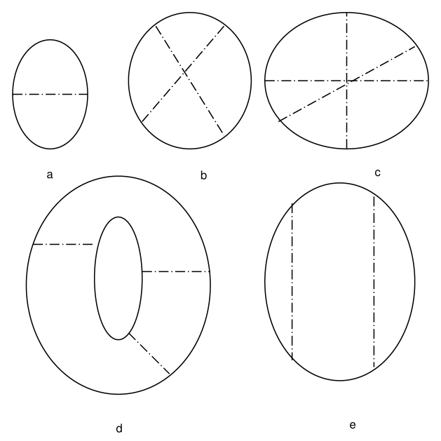
Figure 1: Graphs a, b, c and d are part of the expansion terms in $\Gamma$. Graph e is however reducible and does not show up in the expansion. The solid line represents the propagator $\rho(x,y)$, the dashed line represents the propagator $C(x,y)$.

In section 3, we introduce the finite temperature effective action $\Gamma$. We get this action by a Legendre transformation from $\Omega$. Therefore, we introduce new variables conjugate to the sources. This is exactly the same type of transformation as is used in thermodynamics. At the tree level, the $\Gamma$ functional is simply the action of the system and is related to the free energy of the system. For homogeneous systems, $\Gamma$ is known as the effective potential. In our case $\Gamma$ will be a functional of three variables, the Hartree potential $\varphi(\vec{r})$, the correlation function $C(x,y)$ of the Hartree potential, and the Green’s function $\rho_{\alpha\beta}(x,y)$ of the Fermi field. If the external sources are taken to be instantaneous, the points $x=(\tau_{1},\vec{r_{1}})$ and $y=(\tau_{2},\vec{r_{2}})$, correspond to the same temperature, $\tau_{1}=\tau_{2}$, and the function $\rho_{\alpha\beta}(x,y)$ simply becomes the density matrix of the system. $\alpha$ and $\beta$ are spin indices. Even though it is possible to express the free energy in terms of the density matrix, it makes the manipulations more cumbersome.

In section 4, we solve for $\varphi(x)$ and $C(x,y)$ in terms of $\rho_{\alpha\beta}(x,y)$. We are able to do this simply because in reality $\rho_{\alpha\beta}(x,y)$ is the only independent variable. In this case we get an expression for the effective action $\Gamma$ in terms of the density only. Therefore getting an expression for $\Gamma$ in terms of $\rho_{\alpha\beta}(x,y)$ is the essential result of this work from which other important calculations can be made.

In section 5, we give an explicit expression for the free energy in the homogeneous case in a neutral background. Here we go beyond the RPA results. We show that new diagrams appear at finite temperature. The famous ‘anomalous’ diagram is just one of them (see Fig. 6). An important outcome of this calculation is the disappearance of the $lnT$ behavior in the specific heat that is due to exchange [14] .

In section 6, we treat the zero temperature case. We show explicitly that the anomalous diagrams disappear as they should. Here again we go beyond RPA to include exchange effects on the ring diagrams. We also show that some of the ladder terms are included in our approximation.

In section 7, we continue the treatment started in the previous section and calculate the contribution of the ring diagrams if they include exchange.

In the conclusion, we reexamine the non-homogeneous problem. We show how this method is related to the DFT formalism. In fact it is shown that a statement like the Hohenberg-Kohn theorem is trivially realized in this formalism. Similarly the question of v-representability can be given an affirmative answer within perturbation theory.

2 The Thermodynamic Potential $\mathbf{\Omega}$

In this section, we obtain an expression for the functional $\Omega$ to ‘order’ $\hbar^{2}$. This functional is the logarithm of the partition functional $Z$ of the system in the presence of external sources. The $Z$ functional is written as an integral over all possible allowable paths of the different fields with a weighting factor that depends on the value of the action of the given path. The functional $\Omega$ is simply the generating functional of connected Green’s functions at finite temperature of the fields involved. However because the Coulomb interaction, quartic in the Fermion field, is hard to integrate, we introduce an auxiliary field by means of the well known Hubbard-Stratanovich transformation so that we can avoid the quartic interaction and its nonlocal behavior. In other words, the procedure consists of transforming the problem into one in which the electrons interact locally with a Hartree-type potential. In this treatment, exchange energy terms will show up directly because of the anti-commutation of the Fermi fields, which is built into the calculation as will be described below. The correlation terms are due to the quantum fluctuations around the Hartree potential.

In the following we give an explicit derivation of the terms to order $\hbar^{2}$ in $\Omega$ and no counting will be necessary. What we mean here is that we are including effects of second order in the full Hartree field of the theory. The equation of motion satisfied by $\rho(x,y)$ goes therefore beyond the Hartree-Fock approximation and involves second order exchange effects.

A non-relativistic interacting electron gas in an external potential $V(\vec{x})$ has the following Hamiltonian in the second quantized form:

$$H_{0} =\int d^{3}x\left[-\frac{1}{2}\Psi_{\alpha}^{\dagger}(x)\nabla^{2}\Psi_{\alpha}(x)+V(x)\Psi_{\alpha}^{\dagger}(x)\Psi_{\alpha}(x)\right]$$

$$+\frac{1}{2}\int d^{3}xd^{3}y\frac{1}{|\vec{x}-\vec{y}|}\Psi_{\alpha}^{\dagger}(x)\Psi_{\nu}^{\dagger}(y)\Psi_{\nu}(y)\Psi_{\alpha}(x).$$ (1)

Here, we use units such that $\hbar=m=e=k_{B}=1$ and $\beta\equiv\frac{1}{T}$. $\Psi(x)$ is a two-component temperature-dependent electron field. $\alpha$ and $\nu$ are spin indices, i.e., $\alpha=1$ for spin up and $\alpha=-1$ for spin down. Summation is implicit for repeated indices. In the following $\vec{x}$ will always mean a 3-D space vector. The system is constrained by the condition

$$\int d^{3}x\Psi_{\alpha}^{\dagger}(x)\Psi_{\alpha}(x)=N$$ (2)

where N is the electron number operator which is constant. Therefore the density operator is simply $\Psi_{\alpha}^{\dagger}(x)\Psi_{\alpha}(x).$ Because of this constraint, we prefer to work instead with the following Hamiltonian

$$H=H_{0}-\mu N$$ (3)

where $\mu$ is a Lagrangian multiplier. The electron operator $\Psi(x)$ can be expanded in terms of a complete orthonormal set of one-particle functions $\varphi_{k}(x),$ so we write

$$\Psi(x) =\sum_{k}a_{k}\varphi_{k}(x)\text{ },$$

$$\Psi^{\dagger}(x) =\sum_{k}a_{k}^{\dagger}\varphi_{k}^{\ast}(x)\text{ }.$$ (4)

$a_{k}$ and $a_{k}^{\dagger}$ are annihilation and creation operators. The subscript $k$ includes momentum and spin. The ground state and the excited states can be represented as Slater determinants formed by the wave functions $\varphi_{k}(x)$. In our case, it will be advantageous to take these functions to be self-consistent Hartree eigenfunctions. In the homogeneous case they reduce to plane waves. Since we are going to use a path integral formulation, we give the Lagrangian associated with the Hamiltonian H.

$$L =\int\!d^{3}x\left[i\Psi^{\dagger}(x)\frac{\partial}{\partial t}\Psi(x)+\frac{1}{2}\Psi(x)\nabla^{2}\Psi^{\dagger}(x)-V(\vec{x})\Psi^{\dagger}(x)\Psi(x)+\mu\Psi^{\dagger}(x)\Psi(x)\right]$$

$$-\frac{1}{2}\int d^{3}xd^{3}y\frac{1}{|\vec{x}-\vec{y}|}\Psi^{\dagger}(x)\Psi^{\dagger}(y)\Psi(y)\Psi(x).$$ (5)

So for a system at thermal equilibrium, we have to replace the time component t in the Hamiltonian by $-i\tau$. The partition function $Z$ is as usual defined as a sum over all possible states $\Phi$. In the absence of external sources, we have

$$Z[0] =\sum_{\Phi}\left\langle{\Phi}\,|\,e^{-\beta H}\,|\,{\Phi}\right\rangle$$

$$=N\int D\Psi D{\Psi}^{\dagger}\exp\left({-S[\Psi,\Psi^{\dagger}]}\right)$$ (6)

where N is a normalization constant and the integration measure of the Fermi fields is only defined for fields that satisfy:

$$\Psi(0,x)=-\Psi(\beta,x).$$ (7)

$S[\Psi,\Psi^{\dagger}]$ is the action of the system

$$S[\Psi,\Psi^{\dagger}] =\int_{0}^{\beta}d\tau\,L$$

$$=\int_{0}^{\beta}d\tau\int d^{3}x\;\left\{\Psi^{\dagger}(x)\left[\frac{-\partial}{\partial\tau}+\frac{1}{2}\nabla^{2}+\mu-V(x)\right]\Psi(x)\right\}$$

$$-\frac{1}{2}\int_{0}^{\beta}d\tau\int d^{3}xd^{3}y\;\frac{1}{|\vec{x}-\vec{y}|}\Psi^{\dagger}(x)\Psi^{\dagger}(y)\Psi(y)\Psi(x).$$ (8)

The functional integral for the partition function becomes

$$Z[0] = N\int D\Psi D\Psi^{\dagger}\exp\left\{-\int d\tau_{x}d^{3}x\left[\Psi^{\dagger}(x)\left(\frac{\partial}{\partial\tau}-\frac{1}{2}\nabla^{2}-\mu+V(\vec{x})\right)\Psi(x)\right.\right.$$ (9)

$$\mbox{}\left.\left.+\frac{1}{2}\int_{0}^{\beta}d\tau\;d\tau_{y}\int d^{3}y\frac{\Psi^{\dagger}(x)\Psi(x)\Psi^{\dagger}(y)\Psi(y)}{|\vec{x}-\vec{y}|}\delta(\tau-\tau_{y})\right]\right\}.$$

In writing the last term we made use of the fact that the Fermi fields satisfy a Grassmann algebra. An infinite self-energy term has been dropped from the above expression. Such a term cancels at the end and has no effect on the evaluation of the eigenfunctions or related physical quantities. Now, we set for notational convenience:

$$G^{-1}(x,y)=\left(\frac{\partial}{\partial\tau_{x}}-\frac{1}{2}\nabla^{2}-\mu+V(\vec{x})\right)\delta(x-y)$$ (10)

and

$$A(x,y)=\frac{\delta(\tau_{x}-\tau_{y})}{|\,\vec{x}-\vec{y}\,|}\text{ }.$$ (11)

Before proceeding further, we have to get rid of the quartic term in the Lagrangian. This is done by introducing an auxiliary boson field.
We write

$$Z[0] =N^{\prime}\int D\Psi D\Psi^{\dagger}D\varphi\;\exp\left\{-\int d^{4}xd^{4}y\;\Psi_{\alpha}^{\dagger}(x)G^{-1}(x,y)\Psi_{\alpha}(y)\right.$$

$$\left.-\frac{1}{2}\int d^{4}xd^{4}y\;\varphi(x)A^{-1}(x,y)\varphi(y)+\int d^{4}x\;\varphi(x)\Psi_{\alpha}^{\dagger}(x)\Psi(x)\right\}.$$ (12)

The fourth component is the time component integrated over the proper range. It is easy to see that by using the following formula,

$$\int dx\;e^{-\frac{1}{2}xQx+bx}=(\det Q)^{-\frac{1}{2}}\;e^{\frac{1}{2}bQ^{-1}b}$$ (13)

and integrating over $\varphi$ we get back the original expression for $Z[0]$. The prefactor $N^{\prime}$ is a new normalization constant. The operator $A(x,y)$ is clearly invertible,

$$A^{-1}(x,y)=-\frac{1}{4\pi}\delta(x-y)\nabla^{2}\text{ }.$$ (14)

The non-local character of the Coulomb interaction has been removed by introducing the new bosonic field $\varphi(x).$ It can be shown that $\varphi(x)$ is the Hartree potential by using the new equations of motion derived from the new action of the problem. We also couple the fields to local and non-local sources $J(x),Q(x,y)$ and $B(x,y)$. Now we introduce the functional $\Omega$, a generator of connected Green functions. This is introduced through the normalized partition functional which is now a functional of the external sources. It is given by:

$$Z[J,B,Q]=\exp\left\{-\beta\;\Omega[J,B,Q]\right\}$$ (15)

such that

$$\exp\left(-\Omega[J,B,Q]\right)\int D\Psi D\Psi^{\dagger}D\varphi\;\exp\left(-S[\Psi,\Psi^{\dagger},\varphi]\right)=$$ (16)

$$\int D\Psi D\Psi^{\dagger}D\varphi\exp\left\{-S[\Psi,\Psi^{\dagger},\varphi]+\int d^{4}xd^{4}y\Psi^{\dagger}(x)Q(x,y)\Psi(y)\right.$$

$$\mbox{}+\left.\frac{1}{2}\int d^{4}xd^{4}y\varphi(x)B(x,y)\varphi(y)+\int d^{4}x\varphi(x)J(x)\right\}$$

where we have set $\beta=1$. $S[\Psi,\Psi^{\dagger},\varphi]$ is simply the action of the transformed problem,

$$S[\Psi,\Psi^{\dagger},\varphi] =\int d^{4}xd^{4}y\;\Psi^{\dagger}(x)G^{-1}(x,y)\Psi(y)+\frac{1}{2}\varphi(x)A^{-1}(x,y)\varphi(y)$$

$$-\int d^{4}x\varphi(x)\Psi^{\dagger}(x)\Psi(x)$$ (17)

Now we define three new variables:

$$\frac{\delta\Omega[J,B,Q]}{\delta J(x)}|_{J=B=Q=0}=\left\langle\varphi(x)\right\rangle\equiv\varphi_{c}(x)$$ (18)

$$\frac{\delta\Omega[J,B,Q]}{\delta B(x,y)}|_{J=B=Q=0}=\frac{1}{2}\left\langle\varphi(x)\varphi(y)\right\rangle\equiv\frac{1}{2}\left[\varphi_{c}(x)\varphi_{c}(y)+C(x,y)\right]$$ (19)

$$\frac{\delta\Omega[J,B,Q]}{\delta Q(x,y)}|_{J=B=Q=0}=\left\langle\Psi_{\alpha}^{\dagger}(x)\Psi_{\beta}(y)\right\rangle\equiv\rho_{\alpha\beta}(x,y)$$ (20)

$\varphi_{c}(x)$ is the expectation value of the field $\varphi(x)$ in the ground state. $C(x,y)$ is a correlation function of the field $\varphi(x).$ $\rho_{\alpha\beta}(x,y)$ is the Green function of the Fermi field. $\rho_{\alpha\beta}(x,x)$ is therefore the density of the system. Here and below, the “time” ordering operator is not written explicitly. Therefore terms like $\rho(\vec{x},\vec{y})$ are defined by setting $\tau_{x}-\tau_{y}=0^{+}.$ Note that $C(x,y)$ measures the departure from quasi-independence due to the correlation between the values of the potential at two different locations. The expectation value of the Fermi field $\Psi(x)$ is zero. In the following, we will obtain an explicit expression for $\Omega[J,B,Q]$ to ‘order’ $\hbar^{2}$. Then by solving for $\varphi_{c}(x),C(x,y)$ and $\rho(x,y)$ in terms of $J(x),B(x,y)$ and $Q(x,y)$ we get an expression for the effective action $\Gamma$ which is a functional of the new variables. This will be done in the next section.
Now we turn to determining $\Omega$. First we expand the exponent in the above integral around $\Psi=\Psi^{\dagger}=0$ and $\varphi=\varphi_{0}$ where $\varphi_{0}$ is the configuration of $\varphi$ that extremizes the action S. Therefore, we have

$$\left(A^{-1}+B\right)\varphi_{0}=-J.$$ (21)

It is understood from the above that there is an integration over space and time on the L.H.S. of this expression. We choose from now on not to write integrals explicitly unless there might be some confusion. Now we expand around $\varphi_{0}$, so we write

$$\varphi_{(old)}=\varphi_{(new)}+\varphi_{0}.$$ (22)

Then assuming that the main contribution to the integral comes from the saddle point, we get the following expression for the partition functional:

$$\exp\{-\beta\Omega\} =\exp(-\beta\;S[\varphi_{0}])\;\frac{\det[\widetilde{G}^{-1}+Q]\;\det[A^{-1}+B]^{-\frac{1}{2}}}{\det[G^{-1}]\;\det[A^{-1}]^{-\frac{1}{2}}}\,\Sigma^{-1}$$ (23)

$$\mbox{}\times\,\exp\left[\int D\Psi D\Psi^{\dagger}D\varphi\;\;\Xi\;\left\{\frac{1}{2}e^{2}(\varphi\Psi^{\dagger}\Psi)^{2}\,\;+\ldots\right\}\,\right]$$

where we have defined $\Xi$ and $\Sigma$ to be

$$\Xi =\exp\left[-\Psi^{\dagger}(\widetilde{G}^{-1}+Q)\Psi-\frac{1}{2}\varphi(A^{-1}+B)\varphi\right]$$ (24)

$$\Sigma =\int D\Psi D\Psi^{\dagger}D\varphi\;\exp\left[-\Psi^{\dagger}(G^{-1}+Q)\Psi-\frac{1}{2}\varphi(A^{-1}+B)\varphi\right]$$ (25)

In the above, we have used the fact that

$$\int da\text{ }da^{\dagger}\;e^{-a^{\dagger}Ma}=det\;M$$ (26)

for Grassmann numbers a and a^†, and

$$\int dx\;e^{-\frac{1}{2}xMx}={\left(detM\right)}^{-\frac{1}{2}}$$ (27)

for c-numbers x. The argument of the first term on the right is

$$S[\varphi_{0}]=\frac{1}{2}\varphi_{0}A^{-1}\varphi_{0}+\frac{1}{2}\varphi_{0}B\varphi_{0}+J\varphi_{0}$$ (28)

and

$$\widetilde{G}^{-1}=G^{-1}-\varphi_{0}.$$ (29)

Now using the fact that

$$\det A=e^{Tr\ln A},$$ (30)

we can get an explicit expression for $\Omega[J,B,Q]$:

$$\Omega[J,B,Q] =S(\varphi_{0})-\;Tr\ln[1+G\,\varphi_{0}+GQ]+\frac{1}{2}\;Tr\ln[1+A\,B]$$

$$-\frac{1}{2}\!\int\!D\Psi D\Psi^{\dagger}D\varphi\;(\varphi\Psi^{\dagger}\Psi)^{2}\;\frac{\Xi}{\Sigma}+\ldots$$ (31)

After finding $\Omega$, we now calculate the effective action $\Gamma$. We have to solve for the external sources in terms of the physical variables $\rho$, $C$ and $\varphi_{c}$. This we do in the next section where we find the effective action at finite temperature. However, this treatment applies to zero temperatures too. In this case too, we get an expansion in $\hbar$ . Again $\hbar$ is not a true expansion parameter in the true sense of the word. It is only used as a bookkeeping method for the diagrams included in the expansion of $\Omega$.

3 The Effective Action $\mathbf{\Gamma}$

The effective action is a functional of $\varphi_{c}(x)$, $C(x,y)$, and $\rho(x,y)$, which is obtained by a triple Legendre transformation from $\Omega[J,B,Q]$

$$\Gamma[\varphi_{c},C,\rho] =\Omega[J,B,Q]-\int d^{4}x\;\varphi_{c}(x)J(x)-\frac{1}{2}\int d\text{ }[xy]\;\varphi_{c}(x)B(x,y)\varphi_{c}(y)$$

$$-\frac{1}{2}\int d[xy]\;C(x,y)B(x,y)-\int d\text{ }[xy]\rho(x,y)Q(x,y)\;.$$ (32)

where we have written $d$ $[xyz...]$ for $d^{4}xd^{4}yd^{4}z...$ to simplify the notation. It is understood that the integration over time is carried for $\tau$ in $[0,\hbar\beta]$ for the nonzero temperature case and over all time for the zero temperature case. In this section we will assume we are in the zero temperature regime. However this discussion applies equally well to the nonzero temperature case.

It is easily verified that :

$$\frac{\delta\Gamma[\varphi_{c},C,\rho]}{\delta\varphi_{c}(x)}=-J(x)-\int d^{4}y\;B(x,y)\varphi_{c}(y)$$ (33)

$$\frac{\delta\Gamma[\varphi_{c},C,\rho]}{\delta C(x,y)}=-\frac{1}{2}B(x,y),$$ (34)

and

$$\frac{\delta\Gamma[\varphi_{c},C,\rho]}{\delta\rho(x,y)}=-Q(x,y)\text{ }.$$ (35)

When we turn off the external sources, the above equations give the values of $\varphi_{c},C$ and $\rho$ that minimize the effective action. $\varphi_{c}(x)$ and $C(x,y)$ are really dependent variables since they depend on the auxiliary field $\varphi(x)$, so we should be able in principle to express them in terms of $\rho(x,y)$ which gives us the density.

Now we have to express $J,B$ and $Q$ in terms of $\varphi_{c}$, $C$ and $\rho$. First we note that when $\hbar=0,$ we have

$$\frac{\delta\Omega}{\delta J}=\varphi_{0}.$$ (36)

Hence, we can write

$$\varphi_{0}=\varphi_{c}+\widetilde{\varphi}$$ (37)

where $\widetilde{\varphi}$ is of order $\hbar$. Similarly, we write

$$S(\varphi_{0})=S(\varphi_{c})+\hbar S_{1}.$$ (38)

Now we seek an expression for $\Gamma$ in the form

$$\Gamma=\Gamma_{0}+\hbar\Gamma_{1}+\hbar^{2}\Gamma_{2}.$$ (39)

It then follows that

$$\Gamma_{0}=\frac{1}{2}\varphi_{c}A^{-1}\varphi_{c}.$$ (40)

Now, we find approximate expressions for $B$ and $Q$ in terms of $\varphi_{c},C$ and $\rho$. Using Eq.(31) and Eq.(35), we get the following relation:

$$\rho^{-1}G=1+GQ-eG\varphi_{c}+O(\hbar)\text{ }.$$ (41)

The expression for $B$ is more involved. Again using Eq.(35) and treating $\varphi_{0}$ as a functional of $J$ and $B$, we get:

$$B\,C\,=\,(1-2e\,\rho\,\varphi_{c})\left(1-2\frac{\varphi_{c}\widetilde{\varphi}}{C}\right)^{-1}\,-A^{-1}\,C\text{ }.$$ (42)

Inserting back all these expressions in $\Gamma$, we get for $\Gamma_{1}$

$$\Gamma_{1}=-Tr\;\ln\;(\rho^{-1}G)+\frac{1}{2}Tr\;\ln(C^{-1}A)+\frac{1}{2}Tr\;(A^{-1}C)-Tr\;(\rho\widetilde{G}^{-1})\text{ }.$$ (43)

The terms of order $\hbar^{2}$ are more involved to treat but again straightforward. The steps are similar to those in the case of the effective action with one-point sources only [12]. Actually, it can be shown that the next terms in $\Gamma_{2}$ are the sum of two-particle irreducible diagrams of the theory [8],[9]. Here, we sum only the first two diagrams in this series expansion. Fig. 1 shows the first four diagrams in this expansion. The fifth diagram is not part of the asymptotic expansion of $\Gamma$. These first two diagrams enable us to include first and second order exchange effects. Diagram e is not part of $\Gamma_{2}$ since it is two-particle reducible. However it is one-particle irreducible and it is part of the usual effective action [11],

$$\Gamma_{2} =-\frac{1}{2}e^{2}\int d[xy]\;\rho(x,y)\rho(y,x)C(x,y)$$

$$-\frac{1}{4}e^{4}\int d[xyuv]\;\rho(x,y)\rho(y,u)\rho(u,v)\rho(v,x)C(x,u)C(y,v).$$ (44)

Hence the reducible graphs do not appear in the expansion. It is the term $\Sigma$ that appeared in Eq.(23) that is responsible for excluding such a graph from the expansion. $\Gamma_{2}$ and higher order terms represent vacuum graphs where the propagators are $\rho(x,y)$ and $C(x,y)$ of the Fermi field and the boson field respectively. Therefore to order $\hbar^{2}$, the effective action has the following expression

$$\Gamma[\varphi_{c},C,\rho] =-S(\varphi_{c})+\frac{1}{2}Tr\;\ln AC^{-1}+A^{-1}C$$ (45)

$$-Tr\;\ln\rho^{-1}G+\widetilde{G}^{-1}(\varphi_{c})\rho+\Gamma_{2}[C,\rho],$$

where

$$\widetilde{G}^{-1}(\varphi_{c})=\left(\frac{\partial}{\partial\tau}-\frac{1}{2}\nabla^{2}-\mu+V(x)-\varphi_{c}(x)\right)\text{ }.$$ (46)

The term $\mu\int d^{3}x$ $\rho(x,x)$ cancels the term $\mu N$ in the Hamiltonian H, and therefore it can be handled without difficulty. However, we have to deal with the $\mu$ that appears in the term $Tr\,\ln\rho^{-1}\,G$. This could be removed by a convenient choice of the path of integration in the complex $\omega$-plane. The case $\mu=0$ occurs when there are no charges present. We are dealing with negatively charged electrons bound by a static potential $V(x)$. Therefore bound states appear, with negative energies bounded from below for any physically sensible $V(x)$. In Fig. 2 we show how by going from the $C_{1}$ path, which corresponds to nonzero $\mu$, to the $C_{0}$ path we pick up contributions from the bound states between the two paths, since energies of bound states are poles of the propagator $G^{-1}$ in the complex $\omega$ plane. Note that the eigenvalues $\omega_{k}$ of these states do not take into account correlations due the Coulomb field. Because of the logarithmic operator, there is a cut along the real positive axis. By going back to real time and then Fourier transforming the time dependence, we get

$$\int_{C_{1}}dt\;Tr\ln\left(-i\frac{\partial}{\partial t}-\frac{1}{2}\nabla^{2}-\mu+V(x)\right)$$

$$=\int dt\int_{C_{0}}\frac{d\omega}{2\pi i}\;tr\;\ln\left(-\omega-\frac{1}{2}\nabla^{2}+V\right)\text{ }+\sum_{k}\omega_{k}$$ (47)

where $tr$ applies only to spatial variables. The $\omega_{k}$’s are the eigenvalues of the following equation

$$\left(-\frac{1}{2}\nabla^{2}+V(x)\right)\varphi_{k}(x)=\omega_{k}\varphi_{k}(x)\text{ }.$$ (48)

The single particle functions $\varphi_{k}(x)$ of the potential $V(x)$ are not supposed to be used alone as the starting point for any numerical calculations since they do not take account of the repulsion between electrons. Any numerical calculations will have to start by solving Eq.(56). However, it is clearly advantageous to separate the effect of the external potential $V(x)$. This separation also appears in the usual treatments.

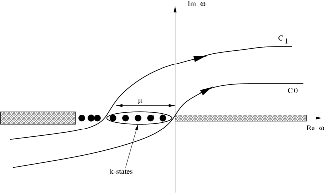
Figure 2: Path of integration used to obtain Eq.(47).

The ground state energy E_g is given in terms of the effective action per unit time. Using the above results, and the fact that the time independent values of $\rho(x,y),C(x,y)$ and $\varphi_{c}(x)$ are defined by setting $\tau_{x}=\tau_{y}=0$, the expression for $E_{g}$ is

$$E_{g}\int dt =\frac{1}{2}\int d[xy]\;\varphi_{c}(x)A^{-1}(x,y)\varphi_{c}(y)\;+\frac{1}{2}Tr\;\ln C\;A^{-1}$$

$$-\frac{1}{2}\int d[xy]\;A^{-1}(x,y)C(y,x)\;-\sum_{\mu<\omega_{k}<0}\omega_{k}\int dt$$

$$-Tr\;\ln\rho G^{-1}+\int d^{4}x\left(\frac{\partial}{\partial\tau_{x}}-\frac{1}{2}\nabla^{2}+V(x)-e\;\varphi_{c}(x)\right)\rho(x,y)|_{\tau_{x}=\tau_{y}}^{x=y}$$

$$+\frac{1}{4}e^{4}\int d[xyuv]\;\rho(x,y)\rho(y,u)\rho(u,v)\rho(v,x)C(x,u)C(y,v)$$

$$+\frac{1}{2}e^{2}\int d[xy]\;C(x,y)\rho(x,y)\rho(y,x)$$ (49)

where we have dropped terms of order higher than $e^{4}$ in $\Gamma_{2}$ for simplicity. This is the full expression for the ground state energy of the system. Here $G^{-1}$ has $\mu$ set to zero. To be able to use this expression for $E_{g}$, more approximations are required. In later sections, we use this expression to find the energy of a homogeneous electron gas both at zero and nonzero temperature. Since $\varphi_{c}$ is a dependent field, then in principle we should be able to solve for $\varphi_{c}$ and $C$ in terms of $\rho$ only. This we do next but only approximately to keep the calculations manageable.

4 The Effective Action as a Functional of $\mathbf{\rho(x,y)}$

In this section, we find an expression for $\Gamma$ solely in terms of the Green’s function $\rho(x,y).$ This is done by finding the expressions for $\varphi_{c}(x)$ and $C(x,y)$, that minimize $\Gamma$, in terms of the density $\rho(x,y).$ For $\varphi_{c}(x)$ we get the following expression:

$$\varphi_{c}(x)=-e\,\int d^{3}y\,\frac{\rho(y,y)}{|\vec{x}-\vec{y}|}\text{ }.$$ (50)

Similarly, minimizing $\Gamma$ with respect to $\rho(x,y)$, we get

$$\delta(x,z)=\left[\frac{\partial}{\partial\tau_{x}}-\frac{1}{2}\nabla^{2}+V(x)-e\;\varphi_{c}(x)\right]\rho(x,z)+e^{2}\int d^{4}y\,\rho(x,y)C(x,y)\rho(y,z)$$ (51)

$$-e^{4}\int d[yuv]\rho(v,u)\rho(u,x)\rho(y,v)\rho(z,y)C(u,y)C(v,x)\>.$$ (52)

Finally, minimizing $\Gamma$ with respect to C, we get

$$\delta(x,z)=\int d^{4}y\left[A^{-1}(x,y)-e^{2}\rho(x,y)\rho(y,x)\right]C(y,z)$$

$$-e^{4}\int d[yvu]C(u,v)C(y,z)\rho(x,u)\rho(u,y)\rho(y,v)\rho(v,x)\>.$$ (53)

To be able to solve for $C(x,y)$ we have to linearize the theory. In the following, we keep terms only to ‘order’ $e^{4}$. Hence, we find that the correlation $C(x,y)$ is given by

$$C(x,z)=A(x,z)+e^{2}\int d[x_{1}x_{2}]\;A(x,x_{1})D(x_{1},x_{2})A(x_{2},z)$$

$$+e^{4}\int d[x_{1}x_{2}x_{1}^{\prime}x_{2}^{\prime}]\;A(x,x_{1}^{\prime})D(x_{1}^{\prime},x_{2}^{\prime})A(x_{2}^{\prime},x_{1})D(x_{1},x_{2})A(x_{2},z)$$

$$+e^{4}\int d[x_{1}x_{2}x_{1}^{\prime}x_{2}^{\prime}]\;\rho(x_{1},x_{1}^{\prime})\rho(x_{1}^{\prime},x_{2})\rho(x_{2},x_{2}^{\prime})\rho(x_{2}^{\prime},x_{1})A(x_{2},x_{1})A(x_{2}^{\prime},z)A(x,x_{1}^{\prime})$$ (54)

where we have set

$$D(x_{1},x_{2})=\rho(x_{1},x_{2})\rho(x_{2},x_{1})\>.$$ (55)

The above equation for $C(x,z)$ can be represented diagrammatically as shown in Fig. 3. The first term is the bare Coulomb potential. The second and the third are the direct and exchange term with one bubble. So far the Fermion propagators are the true propagators in this expansion. In the following we will ignore the corrections with two bubbles and higher.

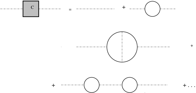
Figure 3: The expansion of the propagator $C(x,z)$ to order $e^{4}$ .

Clearly $C(x,y)$ is the full screened Coulomb potential if all orders of $e^{2}$ are included. Similarly, to order $e^{4}$, the equation satisfied by $\rho(x,z)$ is

$$\left[\frac{\partial}{\partial\tau_{x}}-\frac{1}{2}\nabla^{2}+V(\vec{x})+e^{2}\int dy\frac{\rho(y,y)}{|\vec{x}-\vec{y}|}\right]\rho(x,z)=\delta(x,z)$$

$$-e^{2}\int dy\,A(x,y)\rho(x,y)\rho(y,z)-e^{4}\int d[yx_{1}x_{2}]\;\rho(x,y)\rho(y,z)A(x,x_{1})D(x_{1},x_{2})A(x_{2},y)$$

$$+e^{4}\int d[yx_{1}x_{2}]\;\rho(x_{2},x_{1})\rho(x_{1},y)\rho(x,x_{2})\rho(y,z)A(x_{1},x)A(x_{2},y)\>.$$ (56)

This is obviously the known equation satisfied by the Fermi Green’s functions [11]. The term on the R.H.S. of order $e^{2}$ is an exchange term or Fock term due to the statistics of the electrons. The last two terms of order $e^{4}$ take into account collisions and are equivalent to the usual Born approximation for two-particle Green’s function in scattering theory, Fig. 4.

Figure 4: Born approximation for two-particle Green’s function.

The most likely way to solve these integro-differential equations is by iteration. Using the above equations, we can write an explicit expression for the energy in terms of the full propagator $\rho(x,z)$ of the theory. However, such an expression suffers from the problem of over-counting some of the states of the system. This is mainly due to the fact that $e^{2}$ is not a good expansion parameter. Hence physical arguments are used to discard some terms at this level of approximation and instead include them at higher orders. An expression for the electron propagator in terms of the free propagator is given in Fig. 5 .

Figure 5: Approximate solution to the one-particle Green’s function. The propagators on the right correspond to the free theory.

The corresponding analytical expression can be easily written following usual rules [11]. Here we keep only the first three terms. The second term vanishes in the homogeneous case, the case we are interested in this paper. We expect the expression for the energy, which has not been linearized, to be a good one if we believe that a stationary phase approximation is viable. Without including $\Gamma_{2}$, the expression obtained for the energy is correct with $\rho(x,y)$ the Hartree propagator and $\varphi_{c}(x)$ the Hartree potential. This indicates that a stationary phase approximation is possible and that the higher order correction $\Gamma_{2}$ should be a small perturbation to the Hartree solution. The linearization of the problem must take account of this. Hence, we can justify the validity of the expansion of $\Gamma$ in $\hbar$,

$$\Gamma=\Gamma_{0}+\hbar\Gamma_{1}+\hbar^{2}\Gamma_{2}+...$$ (57)

by the result we get in the end. To second order in $\hbar$, Eq.(54) becomes

$$\int dyA^{-1}(x,y)\;C(y,z)=\delta(x,z)+\hbar e^{2}\int\>dyD(x,y)A(y,z)$$

$$+\hbar e^{4}\int\text{ }d[yuv]\>\rho(x,u)\rho(u,y)\rho(y,v)\rho(v,x)A(u,v)A(y,z)$$

$$-2\hbar^{2}e^{4}\int d[yuv]\rho(x,u)\rho(u,v)\rho(v,y)\rho(y,x)A(u,v)A(y,z)$$ (58)

where $\rho(x,y)$ is the free electron propagator. We have used only a first order approximation to the true propagator to find this equation for $C(x,y)$. Using this equation, we get an expression for the energy to order $\hbar^{2}$ with proper symmetry factors for the diagrams involved in the expansion. Setting $\hbar=1$, we obtain for an interval of time T,

$$T\;E_{g}[\rho]=\frac{e^{2}}{2}\int dx\,dy\;\frac{\rho_{H}(x,x)\rho_{H}(y,y)}{|\vec{x}-\vec{y}|}\,+\,e\int dx\,V(x)\rho_{H}(x,x)$$

$$+\int dx\left(-\frac{1}{2}\nabla^{2}\rho_{H}(x,y)\right)|_{x=y}\;-T\sum_{\omega_{k}>\mu}\omega_{k}$$

$$-\frac{1}{4}\;e^{4}\!\int dx_{1}\,dx_{2}dx\,dy\;\rho_{H}(x_{1},x)\rho_{H}(x,x_{2})\rho_{H}(x_{2},y)\rho_{H}(y,x_{1})A(x,y)A(x_{2},x_{1})$$

$$+\frac{1}{2}\;Tr\,\ln\left[\text{ }\delta(x,z)+e^{2}\int dyA(z,y)D_{H}(x,y)+\right.$$

$$\;e^{4}\int dydx_{1}dx_{2}\;\rho_{H}(x_{1},x)\rho_{H}(x,x_{2})\rho_{H}(x_{2},y)\rho_{H}(y,x_{1})A(x_{2},x_{1})A(y,z)\;-$$

$$\left.2e^{4}\int dydx_{1}dx_{2}\;\rho_{H}(x,x_{1})\rho_{H}(x_{1},x_{2})\rho_{H}(x_{2},y)\rho_{H}(y,x)A(x_{2},x_{1})A(y,z)\;\right]$$

$$-Tr\,\ln\left[\;\delta(x,z)-e^{2}\!\int dy\;\rho_{H}(y,y)\rho_{H}(x,z)A(x,y)-e^{2}\!\int dy\;A(x,y)\rho_{H}(x,y)\rho_{H}(y,z)\right.$$

$$-e^{4}\int dydx_{1}dx_{2}\;\rho_{H}(x,y)\rho_{H}(y,z)\rho_{H}(x_{1},x_{2})\rho_{H}(x_{2},x_{1})A(x_{1},x)A(x_{2},y)$$

$$\left[+e^{4}\int dydx_{1}dx_{2}\;\rho_{H}(x_{2},x_{1})\rho_{H}(x_{1},y)\rho_{H}(x,x_{2})\rho_{H}(y,z)A(x_{1},x)A(x_{2},y)\;\right]$$

$$-e^{2}\!\int dy\;\rho_{H}(y,y)\rho_{H}(x,z)A(y,x)|_{x=z}+e^{2}\int dxdy\;A(x,y)\rho_{H}(x,y)\rho_{H}(y,z)\;|_{x=z}$$

$$-e^{4}\!\int dxdydx_{1}dx_{2}\delta(x-z)\;A(x,x_{1})A(y,x_{2})\rho_{H}(y,z)\rho_{H}(x_{2},x_{1})\rho_{H}(x_{1},y)\rho_{H}(x,x_{2})$$

$$+e^{4}\int dxdydx_{1}dx_{2}\;\delta(x-z)\rho_{H}(x,x_{1})\rho_{H}(x_{1},x_{2})\rho_{H}(x_{2},y)\rho_{H}(y,x)A(x_{2},x_{1})A(y,z).$$ (59)

The trace, $Tr$, acts on x and z. So now we have obtained an expression for the energy in terms of the Green’s functions $\rho(x,z)$ only. This is a major result of the work. As we mentioned above, we solve for $\rho(x,y)$ to order $e^{4}$ by iteration of Eqs.(52-53). The expression for the energy can be solely written in terms of $\rho(x,x)$. However as we stated earlier this is not advantageous and it is better to keep working in terms of $\rho(x,y)$.

We see that the classical Coulomb term and the interaction with the external potential appear naturally in this approximation. They can be easily separated from the full expression for the energy. Another important point is that a gradient of the density also appears naturally within the above expressions. Therefore the kinetic term is treated more accurately in this method compared to the density functional method. By expanding the first logarithm, we immediately obtain the Hartree-Fock exchange term, i.e.,

$$E_{exch}=\frac{1}{2}e^{2}\int dx\,dy\frac{\rho_{H}(x,y)\rho_{H}(y,x)}{|\vec{x}-\vec{y}|}\delta(\tau_{x}-\tau_{y}).$$ (60)

The usual expression for the exchange energy follows trivially from the previous expression upon using the commutation relation of the Fermi field. The infinity arising from this cancels the self-interaction term that was dropped in Eq.(9). There is a similar exchange term that comes from the second logarithmic term . This term is canceled by another similar term outside the logarithm. The usual RPA term is contained in the first logarithm. The new, extra term in the same logarithm provides among other things exchange corrections to the ring diagrams. The higher order exchange diagrams are also included in this approximation. We will say more on this when we treat the homogeneous case in the following sections.
Before we go on to the next section, we should point out that an expression for the energy in terms of the density only is possible in this formalism [13]. The expression is complicated however and does not seem to be useful. We were also able to show that a derivative expansion in terms of the Hartree field is more suitable in our case rather than seeking one in terms of the density. In fact a derivative expansion in terms of the Hartree field seems more appropriate since it is better behaved than the density for problems where the density changes sharply. We hope to address these questions in a later communication.

5 The Fermi Gas at Low Temperature

In this section we use the result found previously to improve on calculations of the exchange energy and ring diagrams made by Isihara and coworkers and others and calculate the specific heat at low temperature [14] . A short review of these calculations appears in Ref.[15] and offers a good comparison of all these methods up to the year 1975. The authors of this paper end with an interesting conjecture which we prove here to be true. The appearance of temperature dependent logarithmic terms in the internal energy found through various calculations is unacceptable. These terms will reappear again in the specific heat and will spoil the observed linear behavior at low temperature. In the past these difficulties were not given close attention. They were either hidden in an effective mass or the expansion was not completely correct as we argue below. The history of this problem dates back to the ’30s when it was first pointed out by Bardeen in Ref.[16] . A preliminary treatment of this work appeared in Ref.[4]. It was argued in Ref.[4] that a correct approximation to the internal energy of a many-particle system up to exchange, i.e., a Hartree-Fock approximation, will automatically include summing an infinite set of diagrams generated by the known “anomalous” diagram, Fig. 6.

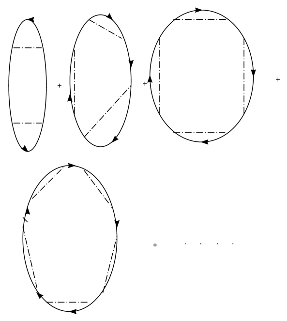
Figure 6: A new infinite set of diagrams at nonzero temperature.

At low temperature, the ring diagrams treated in Ref.[17] are of order $e^{4}$. The exchange energy is of order $e^{2}$. However at nonzero temperature, we have another contribution to order $e^{2}$ that comes from summing an infinite set of diagrams that were never treated before. Therefore the new set can not be ignored in any finite temperature treatment. We show below that taking these diagrams into account is exactly what is needed to solve the anomaly in the exchange energy at finite temperature. The grand partition function $Z$ of the system is given in this case by the following expression:

$$Z=\exp(-\beta\Omega)=Tr\exp\left(-\beta\left[\left(\mathrm{H-\mu N}\right)+j\varphi+\frac{1}{2}\varphi\mathrm{B\varphi+\psi^{{\dagger}}Q\psi}\right]\right)\text{ }.$$ (61)

The thermodynamical potential is a functional of $j$, $B$ and $Q$ but it is a function of the variables $\mu,$ $T$ and $V$. To get the free energy $F[\rho,\varphi_{c},\Delta]$ we make the following triple Legendre transformation

$$F[\rho,\varphi_{c},\Delta]-\mu\,N=\Omega[j,B,Q]-j\varphi_{c}-\frac{1}{2}\varphi_{c}B\varphi_{c}-\rho Q-\Delta B$$ (62)

where $\rho$, $\varphi_{c}$ and $\Delta$ are defined as before, Eqs.(18-20). We have seen that ${F}$ ($E$ at $T=0$) can be calculated perturbatively by expanding the exponent around the classical Hartree potential in a neutral background, i.e., with no external potential. The coefficients of this expansion are expressible in terms of Feynman diagrams. Here in this section we keep only the first two terms of the expansion, in other words we only include the first diagram in Fig. 1.

The equation of motion satisfied by $\rho(x,x^{\prime})$ is given by:

$${\left(\frac{\partial}{\partial\tau}-\frac{1}{2}{\nabla}_{x}^{2}-\mu\right)\rho(x-y)}=\delta(x-y)-e^{2}\int dz\rho(x-z)\rho(z-y)\Delta(z-x)\text{ },$$ (63)

where $\Delta(z-x)$ is the bare Coulomb potential to first approximation. It must be pointed out again that a full solution to $\Delta(z-x)$ gives the expected shielded potential. An approximate solution to the full linearized equation for $\Delta(z-x)$ was first given in Ref.[18]. We must stress however that in what follows we use only the zero order solution to $\Delta(z-x).$ In this case the above equation is the Hartree-Fock approximation to the equation of motion for the one-particle Green’s function $\rho(x-y)$ at finite temperature [19]. The final expression that we are after is that for the thermodynamic potential $\Omega(\mu,T,V)$. Hence within the above approximation, the expression for the thermodynamic potential has the following form:

$$\Omega =\Omega_{0}+\Omega_{ex}+\frac{1}{2}Tr\left\{\ln\left[\delta(x-y)+e^{2}\Re(x-y)\right]-e^{2}\Re(x-y)\right\}$$

$$-Tr\left\{\ln\left[\delta(x-y)-e^{2}\Im(x-y)\right]+e^{2}\Im(x-y)\right\}$$ (64)

where the functions $\Re(x-y)$ and $\Im(x-y)$ are given by

$$\Re(x-y)=\int_{0}^{\beta}d\tau\int d^{3}zA(y-z)\rho(x-y)\rho(z-x)$$ (65)

and

$$\Im(x-y)=\int_{0}^{\beta}d\tau\int d^{3}zA(x-z)\rho(z-x)\rho(y-z)\>.$$ (66)

The term $\Omega_{0}$ is the free contribution, $\Omega_{ex}$ is the usual first order exchange term, the third term represents the usual ring diagrams and the last term represents a new series of diagrams shown in Fig. 6. The function $A(x-y)$ is the bare Coulomb potential and $\rho(x-y)$ is the free one-particle Green’s function at finite temperature. It should be stressed from the above treatment that the new diagrams are necessary for the consistency of our approximations. The first diagram of the new set of diagrams was treated previously by Isihara and Kojima in Ref.[20] in a calculation of the specific heat. Here we do the same calculation again but taking into account the full sequence of the new diagrams. The method used by these authors differs from ours, however they are both based on path integrals and both start from a partition function. In this sense our methods are more exact than those that start from a zero temperature treatment like Gell-Mann’s treatment in Ref.[21] or those based on a phenomenological theory like Landau’s. The authors of Ref.[15] claim at the end of their paper that screening is probably not needed to have a reasonable answer for the specific heat. Here we show that indeed this claim is true. It is well known that the exchange energy has an odd $\ln T$ behavior that ends up contributing a $T\ln T$ term to the specific heat. This is obviously not reasonable for low temperatures. The exchange energy at low temperature is given by [22],[1] :

$$\Omega_{ex}=-V\frac{e^{2}m^{2}}{2\pi^{2}}\left\{\frac{2}{\pi}\mu^{2}-\frac{\pi}{3\beta^{2}}(1+\ln\beta\mu-\gamma)\right\}\>.$$ (67)

Now we give the contribution due to the ring diagrams at finite temperature [23]. This contribution is given by

$$R\;=\frac{1}{2}Tr\left\{ln\left[\delta(x-y)+e^{2}\Re(x-y)\right]-e^{2}\Re(x-y)\right\}.$$ (68)

In momentum representation, this is given by

$$R\;=\frac{V}{2\beta}\,\sum_{n=-\infty}^{n=\infty}\frac{4\pi}{(2\pi)^{3}}\int_{0}^{\infty}\,p^{2}\,dp\;\left[\ln\left\{1+e^{2}\Re(p,\omega_{n})\right\}-e^{2}\Re(p,\omega_{n})\right]$$ (69)

where p represents momentum and $\omega_{n}=\frac{(2n+1)\pi}{\beta}$, $n=0,\pm 1,\pm 2,\ldots$. The function $\Re(p,\omega_{n})$ is given by:

$$\Re(p,\omega_{n})\;=\;\frac{2}{(2\pi)^{3}p^{2}}\!\int\!d\vec{q}\frac{\frac{1}{2}(\vec{p}+\vec{q})^{2}-\frac{1}{2}\vec{q}^{2}}{\omega_{n}^{2}+\left(\frac{1}{2}(\vec{p}+\vec{q})^{2}-\frac{1}{2}\vec{q}^{2}\right)^{2}}(f(\vec{q})-f(\vec{p}+\vec{q})).$$ (70)

The function $f(\vec{q})$ is the Fermi-Dirac function,

$$f(\vec{q})\;=\;\frac{1}{1+\exp\left[\beta(\frac{q^{2}}{2}-\mu)\right]}.$$ (71)

Therefore the finite temperature contribution of the ring diagrams to leading order in ${\frac{1}{\eta^{2}}}$, $\eta=\beta\mu$, and for high density is given by

$$R\,=\,N(0.0622\ln r_{s}-0.142)+0.0181\,\mathit{N}(T)\;\mu\;(\frac{\alpha r_{s}(T)}{\eta})^{2}\text{ }.$$ (72)

Here $N$ is the total number of particles, which is a constant. All the other variables are defined as follows:

$$\alpha=(\frac{4}{9\pi})^{\frac{1}{3}},\>\>r_{s}(T)=\frac{me^{2}}{\alpha\hbar^{2}k_{F}},\>\>\,a_{0}=\frac{\hbar^{2}}{me^{2}},\>\>\mathit{N}(T)=\frac{V}{\frac{4\pi}{3}r_{s}(T)^{3}a_{0}^{3}}\>.$$ (73)

To obtain this answer, we have used explicitly the fact that $r_{s}$ is small to simplify the calculation. It is however important to stress that this approximation does not affect our final result regarding the $\ln T$ terms in the specific heat. Obviously our result will not apply even to $r_{s}\approx 1$.

The contribution of the new set of diagrams, Fig. 6, is given by :

$$\mathcal{A} =Tr\left\{\text{ }\ln\left[\text{ }\delta(x-y)-e^{2}\Im(x-y)\right]+e^{2}\Im(x-y)\right\}$$

$$=\frac{2V}{\beta}{\sum_{n=-\infty}^{\infty}}\frac{4\pi k_{F}^{3}}{{\ (2\pi)}^{3}}\int_{0}^{\infty}x^{2}dx\left[\>\ln\left(1-e^{2}\Im(x,\omega_{n})\right)+e^{2}\Im(x,\omega_{n})\right].$$ (74)

Here $x=\frac{k}{k_{F}}$ is the normalized momentum and $\omega_{n}=\frac{(2n+1)\pi}{\beta}$ for $n=0,\pm 1,\pm 2,...$. The function $\Im(x,\omega_{n})$ is given by :

$$\Im(x,\omega_{n})=\frac{1}{\pi^{2}}\rho(x,\omega_{n})\int d^{3}\vec{p}\frac{1}{1+\exp(\eta(\frac{p^{2}}{2}-1))}\frac{1}{\mid\vec{p}-x\vec{k_{F}}\mid^{2}}$$ (75)

with

$$\rho(k,\omega_{n})=\frac{i}{i\omega_{n}-(\frac{k^{2}}{2}-\mu)}$$ (76)

and $\eta=\beta\mu$. The mass of the electron is taken to be m=1. The calculation is carried out for large $\eta$, i.e. for low temperature. Again here we used explicitly that $r_{s}$ is a small parameter. After some lengthy calculations, we get the following explicit expression for $\mathcal{A}$ to order $\frac{1}{\eta^{2}}$ :

$$\mathcal{A}=\frac{2e^{2}V}{\pi^{3}}k_{f}^{4}\left\{\frac{\pi^{2}}{24\eta^{2}}\left(\zeta+\frac{1}{2}\ln\eta\right)\right\}$$ (77)

where $\zeta$ is a constant.

There are two things to note. First there is no zero temperature contribution due to these diagrams, which is as it is supposed to be. Second, the sum of the new diagrams gives an answer which is of order $e^{2}$, that is it has the same order as the first order exchange energy even though the terms in the sum are of order at least $e^{4}$. This is the reason we believe that an expansion in $e^{2}$ did not pick up this new infinite set of diagrams. It is also of interest to note that the ring diagrams add up to a term of order $e^{4}$. Now a close comparison of the three terms shows that the $\ln T$ term in the exchange energy gets cancelled by the one found from the new set of diagrams. The ring diagrams contribute a temperature dependent term of order $e^{4}$ and hence they are not needed to solve the $\ln T$-term in the exchange. In other words screening does not play any role in this odd behavior of the exchange energy or for that matter of the specific heat as we show next.

The specific heat formula is:

$$C_{V}\,=\,-T\frac{\partial^{2}F}{\partial T^{2}}$$ (78)

where the free energy $F$ is given by, $F(T,V,N)=\Omega+\mu N$. Using standard techniques [24], we calculate the contribution of all of the above terms to the specific heat. To first order in $\frac{1}{\beta^{2}}$, we have [23] :

$$F(T,V,N)\,=\,F_{0}(T,V,N)+\frac{k^{2}T^{2}}{\mu_{0}^{2}}\left(-\frac{20.19}{r_{s}}-0.077\ln r_{s}+0.184\right)$$ (79)

where $F_{0}$ is the free energy of a free electron gas. Therefore, if $C_{V}^{0}$ is the specific heat for the ideal Fermi gas, we get for the specific heat at low temperatures and high densities the expression,

$$\frac{C_{V}}{C_{V}^{0}}\,=\,1.00+0.185r_{s}-r_{s}^{2}(0.0017-0.0007\ln r_{s})\text{ }.$$ (80)

The constants $\zeta$ and $\gamma$ are approximately equal to 8.0 and 2.0, respectively. Now we turn again to the zero temperature case and calculate the correction due to the inclusion of diagram $b$, Fig. 1, in the expansion of the energy.

6 The Homogeneous Electron Gas at Zero
Temperature

In this section we apply the main result of section 4, the expression for the energy, to the homogeneous case at zero temperature. We assume that there is a background of positive charge of equal magnitude to the average density of the electron gas. Hence the system is neutral. The literature on this problem of the calculation of the correlation energy is huge. The most complete treatment, so far as we are aware, was given by Bishop and Luhrmann and it was restricted to zero temperature effects [25] . Since the system is homogeneous, the final expression for the energy will be given in momentum space. The Green’s function that will be used in the following is the solution to the first iteration of the nonlinear equation satisfied by $\rho(x,y)$. Since there is no external potential, the input Green’s function is that of a free electron gas. The energy expression is given in imaginary time, hence we use the following expression for the free Green’s function

$$\rho_{0}(\omega,k)=\frac{1}{-i\omega+\frac{1}{2m}k^{2}-\mu}\>\>.$$ (81)

In this section and the next, the electron Green’s function definition differs by a factor of i from the one given before. In terms of $\rho_{0}(x,y)$, the ground state energy is given by the following, omitting the subscript 0 for simplicity,

$$-T\;E_{gs}=\int d^{4}x\,\left(\frac{1}{2}i\nabla^{2}\rho(x,y)\right)_{x=y}\text{ }$$

$$\text{\ }+\frac{e^{4}}{4}\int dx\,dz\,\delta(x-z)\;\mathcal{M}(x,z)+\frac{e^{2}}{2}\int dx\,dy\;\rho(x,y)\rho(y,x)A(x,y)$$

$$-\frac{1}{2}Tr_{(x,z)}\text{ \ }\ln\text{ }\left[\delta(x,z)-e^{2}\mathcal{H}(x,z)+\text{ }e^{4}\,\mathcal{M}(x,z)-2\text{ }e^{4}\Pi(x,z)\text{ }\right]\text{ \ }$$

$$+Tr_{(x,z)}\text{ \ }\ln\left[\delta(x,z)-e^{2}\mathcal{K}(x,z)-e^{4}\;\Sigma(x,z)\text{ }\right]\text{ \ \ \ \ \ \ \ \ \ \ \ \ \ \ \ \ \ \ \ \ \ \ \ \ \ \ \ \ \ \ }$$

$$+\int dx\,dz\,\delta(x-z)\;\left\{\frac{e^{2}}{2}\mathcal{H}(x,z)-\frac{e^{4}}{2}\mathcal{M}(x,z)+e^{4}\Sigma(x,z)+e^{4}\Pi(x,z)\right\},$$ (82)

where

$$\mathcal{M}(x,z)=\int dy\,dx_{1}\,dx_{2}\,\rho(y,x_{2})\rho(x_{2},x)\rho(x,x_{1})\rho(x_{1},y)A(x_{1},x_{2})A(y,z)\text{ },$$ (83)

$$\mathcal{H}(x,z)=\int dy\,A(z,y)D(x,y)\text{ },$$ (84)

$$\Pi(x,z)=\int dy\,dx_{1}\,dx_{2}\,\rho(y,x)\rho(x,x_{1})\rho(x_{1},x_{2})\rho(x_{2},y)A(x_{1},x_{2})A(y,z)\text{ },$$ (85)

$$\mathcal{K}(x,z)=\int dy\,A(x,y)\rho(x,y)\rho(y,z)\text{ },$$ (86)

$$\Sigma(x,z)=\Sigma_{1}(x,z)-\Sigma_{2}(x,z)\text{ },$$ (87)

$$\Sigma_{1}(x,z)=\int dy\,dx_{1}\,dx_{2}\,\rho(x,y)\rho(y,z)\rho(x_{1},x_{2})\rho(x_{2},x_{1})A(x,x_{1})A(x_{2},y)\text{ },$$ (88)

$$\Sigma_{2}(x,z)=\int dy\,dx_{1}\,dx_{2}\,\rho(x,x_{2})\rho(x_{2},x_{1})\rho(x_{1},y)\rho(y,z)A(x_{1},x)A(x_{2},y)\text{ }.$$ (89)

The above equation, Eq.(82), is simply Eq.(59) taking into account of the fact that $\rho(x,x)$ gets canceled by an equal and opposite charge. Because of the transitional invariance of the system, we can write a simple expression for the correlation energy in the momentum representation,

$$E_{c} =\frac{1}{4}e^{4}V\int\prod_{i=1}^{3}\frac{d^{3}p_{i}}{(2\pi)^{3}}\frac{d\omega_{i}}{2\pi}A(p_{1}-p_{2})A(p_{2}-p_{3})\rho(p_{1})\rho(p_{2})\rho(p_{3})\rho(p_{1}-p_{2}+p_{3})$$

$$+\frac{1}{2}V\int\frac{d^{3}p}{(2\pi)^{3}}\frac{d\omega}{2\pi}\left\{\ln\left[1+e^{2}\mathcal{H}(p)+e^{4}\mathcal{M}(p)-2e^{4}\Pi(p)\right]-e^{2}\mathcal{H}(p)-e^{4}\mathcal{M}(p)+2e^{4}\Pi(p)\right\}$$

$$-V\int\frac{d^{3}p}{(2\pi)^{3}}\frac{d\omega}{2\pi}\left\{\;\ln\left[1-e^{2}\mathcal{K}(p)-e^{4}\Sigma(p)\right]+e^{2}\mathcal{K}(p)+e^{4}\Sigma(p)\;\right\}\;.$$ (90)

Since the ring diagrams are part of $E_{c}$, this will be the first test to see if our expansion gives the correct leading result. First we show how this equation follows from Eq.(82). We start by letting

$$\mathcal{H}(x,z)=-\int\,dy\>D(x,y)A(y,z)$$ (91)

or, since the system is homogeneous, we can write instead

$$\mathcal{H}(x-z)=\int dy\,D(x-y)A(y-z).$$ (92)

Next, we rewrite $D(x-y)$ and $A(x-z)$ in terms of their corresponding Fourier transforms, i.e.,

$$D(x-y)=\int\frac{dk}{(2\pi)^{4}}\;\exp[ik\cdot(x-y)]D(k)$$ (93)

and

$$A(y-z)=\int\frac{dq}{(2\pi)^{4}}\;\exp[iq\cdot(y-z)]A(q)\text{ }.$$ (94)

Hence, by convolution we have,

$$\mathcal{H}(p)\,=\,(A\,\star\,D)\;(p)\text{ },$$ (95)

however since

$$D(p)=\int\frac{dq}{(2\pi)^{4}}\text{ }\rho(p+q)\,\rho(q),$$ (96)

it follows then that,

$$\mathcal{H}(p)\,=\,A(p)\,\int\frac{dq}{(2\pi)^{4}}\,\rho(p+q)\rho(q).$$ (97)

After using the expressions for the propagators, we end up with the following expression for $\mathcal{H}(p)$

$$\mathcal{H}(p)=\frac{4\pi}{p^{2}}\!\int\!\frac{dq}{(2\pi)^{4}}\,\frac{1}{-i\bar{\omega}+\frac{1}{2}\,{\vec{q}}^{2}-\mu}\;\frac{1}{-i(\bar{\omega}+\omega)+\frac{1}{2}\,(\vec{p}+\vec{q})^{2}-\mu}$$ (98)

with $q=(\bar{\omega},\vec{q})$. Integrating first over $\bar{\omega}$ in the complex plane, we find that

$$\mathcal{H}(p)=-2e^{2}\frac{4\pi}{p^{2}}\!\!\int\!\!\frac{d\vec{q}}{(2\pi)^{3}}\frac{\left(\frac{1}{2}(\vec{p}+\vec{q})^{2}-\frac{1}{2}\vec{q}^{2}\right)\left(\Theta(\mu-\frac{1}{2}\vec{q}^{2})-\Theta(\mu-\frac{1}{2}(\vec{p}+\vec{q})^{2})\right)}{\omega^{2}+\left(\frac{1}{2}(\vec{p}+\vec{q})^{2}-\frac{1}{2}\vec{q}^{2}\right)^{2}}$$ (99)

where we added a factor of $2$ to account for spin. This term $\mathcal{H}(p)$ will prove to be all that is needed to reproduce the known RPA result. All other terms that appear in the energy expression are new additions to the correlation. Before showing this explicitly , we give the expressions for the remaining terms $\mathcal{K}(p)$, $\mathcal{M}(p)$, $\Pi(p)$, $\Sigma_{1}(p)$, $\Sigma_{2}(p)$ and $\Sigma(p)$.

$$\mathcal{K}(p)=\rho(p)\int\frac{dq}{(2\pi)^{4}}\text{ }\rho(p+q)\text{ }A(q)$$ (100)

$$\mathcal{M}(p)=A(p)\int\frac{dk_{1}}{(2\pi)^{4}}\frac{dk_{2}}{(2\pi)^{4}}\rho(k_{1})\rho(k_{1}+p)\rho(k_{2})\rho(k_{2}-p)A(k_{1}-k_{2}+p)\text{ },$$ (101)

$$\Pi(p)=A(p)\int\frac{dk_{1}}{(2\pi)^{4}}\frac{dq}{(2\pi)^{4}}\rho(k_{1})\rho(k_{1}-p)\rho(k_{1}-p-q)A(q)\text{ },$$ (102)

$$\Sigma_{1}(p)=\rho(p)\int\frac{d^{4}p_{1}}{(2\pi)^{4}}\frac{d^{4}p_{2}}{(2\pi)^{4}}\,\rho(p_{1})\rho(p_{2})\rho(p_{2}+p_{1}-p)A(p_{2}-p)A(p-p_{1})\text{ },$$ (103)

$$\Sigma_{2}(p)=\rho(p)\int\frac{d^{4}p_{1}}{(2\pi)^{4}}\frac{d^{4}p_{2}}{(2\pi)^{4}}\,A^{2}(p_{1})\rho(p-p_{1})\rho(p_{1}+p_{2})\rho(p_{2})$$ (104)

and

$$\Sigma(p)=\rho(p)\int\frac{d^{4}k_{1}}{(2\pi)^{4}}\frac{d^{4}k_{2}}{(2\pi)^{4}}\rho(k_{1})\rho(k_{2})\rho(k_{2}+k_{1}-p)\left[A(k_{1}-p)^{2}-A(p-k_{2})A(p-k_{1})\right]\text{ }.$$ (105)

The Fourier transform $A(p)$ is given as usual by

$$A(\,p\,)\;=\;\frac{4\,\pi}{|\,\vec{p}\,|^{2}}\>.$$ (106)

The terms in Eq. (90) have the following meaning after we expand the $\ln$-terms. The first term represents the second order exchange term, Fig. 7.

Figure 7: Second order exchange diagram in Eq. 90.

The term $\mathcal{H}(p)$ is responsible for generating the ring diagrams, Fig. 8.

Figure 8: Ring diagrams generated by $\mathcal{H}(p)$ in Eq. (90).

The term $\mathcal{M}(p)$ is responsible for generating some of the ring diagrams with exchange. The cross terms give the remaining ring diagrams with exchange, Fig. 9.

Figure 9: Diagrams that appear in the first ln term in Eq.( 90).

The $\Pi(p)$ term generates ring diagrams with a self-energy insertion in each ring, fig. 10.

Figure 10: Ring diagrams generated by $\Pi(p)$ in Eq. (90).

Hence the terms in the first $ln$ should contribute the most. Some of the terms that appear upon expansion of the second $\ln$ term are shown in Fig. 11.

Figure 11: Diagrams that appear in the second ln term in Eq.( 90).

The term $\mathcal{K}(p)$ generates the so called ‘anomalous’ diagrams, Fig. 6. The term $\Sigma_{1}(p)$ generates ladder terms like those in Figs. 12 and  13.

Figure 12: A term of order $e^{4}$ that is due to $\Sigma_{1}$. Both representations are equivalent. Initially two particles interact with each other with one of them going back to its initial state while the other one interacts with a third particle before both returning to their corresponding initial states.

Figure 13: Some of the ladder diagrams due to $\Sigma_{1}$.

$\Sigma_{2}(p)$ generates terms like those in Fig. 14.

Figure 14: Few terms that appear due to $\Sigma_{2}$.

Cross terms of the last two terms are shown in Fig. 15.

Figure 15: A term that is both due to $\Sigma_{1}$ and $\Sigma_{2}$. Here three particles are interacting pairwise with two of the three particles exchanging states.

Diagrams that appear in Fig. 16 are important in a nonhomogeneous medium and must be accounted for since they no longer vanish. They arise whenever we have a $\rho(x,x)$ term in the expression for energy, Eq.(59).

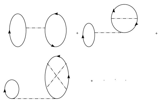
Figure 16: Coulomb interactions that must be taken into account in inhomogeneous media. These diagrams vanish in the homogeneous case.

Normalizing the momentum with respect to $k_{F}$, the Fermi momentum, the explicit expression for the correlation energy per particle in Rydbergs (Ryd.) has the following form,

$$\frac{E_{c}}{N}=\frac{3}{16\pi^{5}}\int d^{3}q\,d^{3}p_{1}\,d^{3}p_{2}\frac{\theta(1-p_{2})\theta(1-p_{1})\theta(E_{q_{1}}-1)\theta(E_{q_{2}}-1)}{q^{2}(q+p_{{}_{1}}-p_{{}_{2}})^{2}(q^{2}+q\cdot p_{1}-q\cdot p_{2})}$$ (107)

$$\mbox{}+\frac{3}{4\pi\alpha^{2}r_{s}^{2}}\int_{-\infty}^{\infty}dx\int_{0}^{\infty}dy\>y^{2}\left\{\ln\left[1+\mathcal{H}(x,y)+\mathcal{M}(x,y)-2\Pi(x,y)\right]\right.$$

$$\left.-\mathcal{H}(x,y)-\mathcal{M}(x,y)+2\Pi(x,y)\right\}$$

$$-\frac{3}{2\pi\alpha^{2}r_{s}^{2}}\!\int_{-\infty}^{\infty}\!dx\int_{0}^{\infty}\!dy\>y^{2}\left\{\ln\left[1+\mathcal{K}(x,y)+\Sigma(x,y)\right]-\mathcal{K}(x,y)-\Sigma(x,y)\right\},$$

where we have set $E_{q_{1}}=|\vec{q}+\vec{p}_{1}|$ and $E_{q_{2}}=|\vec{q}-\vec{p}_{{}_{2}}|$.
For convenience, we set

$$\frac{E_{c}}{N}=I_{1}\,+\,I_{2}\,+\,I_{3}$$ (108)

where $I_{1}$, $I_{2}$, and $I_{3}$ are the first, the second and the third integrals, respectively. Expressions for few of the functions that appear above are given below. The functions $\mathcal{K}(x,y)$, $\mathcal{H}(x,y)$ and $\Sigma_{1}(x,y)$ are given by,

$$\mathcal{K}(x,y)\,=\,\frac{4\alpha r_{s}g(y)}{\pi(-ix+y^{2}-1)},$$ (109)

$$\mathcal{H}(x,y)\,=\,-e^{2}\,A(x,y)D(x,y)$$ (110)

or more explicitly, we have

$$\mathcal{H}(x,y) =\frac{2\alpha r_{s}}{\pi y^{2}}\left[1+\frac{1}{8y^{3}}\left(x^{2}+4y^{2}(1-\frac{y}{2})(1+\frac{y}{2})\right)\ln\left(\frac{(\frac{x}{2})^{2}+y^{2}(1+\frac{y}{2})^{2}}{(\frac{x}{2})^{2}+y^{2}(1-\frac{y}{2})^{2}}\right)\right.$$

$$\left.-\frac{x}{2y}\left(\arctan\left(\frac{y(\frac{y}{2}+1)}{\frac{x}{2}}\right)-\arctan\left(\frac{y(\frac{y}{2}-1)}{\frac{x}{2}}\right)\right)\text{ }\right]$$ (111)

and

$$\Sigma_{1}(x,y)=\frac{16\alpha^{2}r_{s}^{2}}{(2\pi)^{4}}\!\int\!d^{3}k_{1}d^{3}k_{2}\text{ }g(x,y,k_{1},k_{2})$$ (112)

where

$$g(x,y,k_{1},k_{2})=\frac{1}{|\vec{y}-\vec{k}_{1}|^{2}}\frac{1}{|\vec{y}-\vec{k}_{2}|^{2}}\times\frac{\left(\theta(1-k_{1})-\theta(1-k_{12})\right)\left(\theta(k_{1}-E^{\prime})-\theta(1-k_{2})\right)}{(-ix+y^{2}-1)(ix-k_{2}^{2}-k_{1}^{2}+E^{\prime}-1)}$$

$\theta(x)$ is the step function. $E^{\prime}$, $g(y)$ and $\alpha$ are given by

$$E^{\prime}=|\vec{k}_{1}+\vec{k}_{2}-\vec{y}|^{2},$$ (113)

$$\alpha=\left(\frac{4}{9\pi}\right)^{\frac{1}{3}},$$ (114)

and

$$g(y)=1+\frac{1-y^{2}}{2y}\ln\left|\frac{1+y}{1-y}\right|\text{ }.$$ (115)

The Gell-Mann-Brueckner term can be isolated from the full expression for the correlation, Eq.( 107), by rewriting the second integral, $I_{2}$, in the following way:

$$I_{2}=I_{2}^{ring}+I_{2}^{exch}+I_{2}^{seRing}$$ (116)

where

$$I_{2}^{ring} =\frac{3}{4\pi}\frac{1}{r_{s}^{2}\alpha^{2}}\int_{-\infty}^{+\infty}dx\int_{0}^{\infty}dy\,\>y^{2}\left\{\ln\left[1+\mathcal{H}(x,y)\right]-\mathcal{H}(x,y)\right\}\>$$ (117)

$$I_{2}^{exch} =\frac{3}{4\pi}\frac{1}{r_{s}^{2}\alpha^{2}}\int_{-\infty}^{\infty}dx\int_{0}^{\infty}dy\>y^{2}\left\{\ln\left[1+\frac{\mathcal{M}(x,y)}{1+\mathcal{H}(x,y)}\right]-\mathcal{M}(x,y)\right\}.$$ (118)

$I_{2}^{seRing}$ is what is left of $I_{2}-I_{2}^{ring}-I_{2}^{exch}$. The term $I_{2}^{ring}$ is indeed the full expression for the RPA term $\frac{1}{N}E_{c}^{RPA}.$ By taking the limit $r_{s}\rightarrow 0$ and $y<1$, it reduces to the Gell-Mann-Brueckner result [17]:

$$\frac{E_{c}^{RPA}}{N}\approx 0.0622\ln r_{s}-0.142+\ldots$$ (119)

as we show next. Going back to the expression for $\mathcal{H}(p)$, Eq.( 99), we have

$$I_{2}^{ring}=\frac{1}{2}\int\frac{d^{3}k}{(2\pi)^{3}}\int\frac{d\omega}{2\pi}\left[\ln\left(1+\mathcal{H}(k,\omega)\right)-\mathcal{H}(k,\omega)\right]$$ (120)

with $\mathcal{H}(k,\omega)$ defined to be

$$\mathcal{H}(k,\omega)=2e^{2}\frac{4\pi}{k^{2}}\!\int\!\frac{d^{3}p}{(2\pi)^{3}}\,\frac{\left(\frac{1}{2}(\vec{p}+\vec{k})^{2}-\frac{1}{2}\vec{p}^{2}\right)}{\omega^{2}+\left(\frac{1}{2}(\vec{p}+\vec{k})^{2}-\frac{1}{2}\vec{p}^{2}\right)}\left(\theta(\mu-\frac{p^{2}}{2})-\theta(\mu-\frac{1}{2}(\vec{p}+\vec{k})^{2})\right)\text{ }.$$ (121)

Now we set,

$$\mathcal{H}(k,\omega)=\frac{2e^{2}}{(2\pi)^{3}}\,\frac{4\pi}{k^{2}}\left(H_{1}(k,\omega)+H_{2}(k,\omega)\right)$$ (122)

Terms other than $I_{2}^{ring}$ in Eq.( 107) provide new correlations to the RPA-term. The first term in Eq.( 107 ), as we mentioned above, is the second order exchange term and has been evaluated exactly in Ref.[26],

$$E_{c}^{2exch} =\frac{1}{3}\ln 2-\frac{3}{2\pi^{2}}\zeta(3)$$ (123)

$$\simeq 0.04836\text{ \ }Ryd.$$

To compare our expansion to others we calculate the term that is equivalent to the RPA calculation. We start by evaluating the integral $H_{1}$. After integrating the angular variables, we have

$$H_{1}(\omega,k)=\pi\int_{0}^{k_{F}}\frac{p\,dp}{k}\,\ln\left[\;\frac{\omega^{2}+(pk+\frac{1}{2}k^{2})^{2}}{\omega^{2}+(-pk+\frac{1}{2}k^{2})^{2}}\;\right]\text{ }.$$ (124)

This integral can be easily performed over p. We get after that

$$H_{1}(\omega,k) =\frac{\pi}{k^{3}}\left\{\>\frac{1}{2}\ln\left[\;\omega^{2}+k^{2}(k_{F}+\frac{k}{2})^{2}\right]\left[\omega^{2}+k^{2}(k_{F}-\frac{k}{2})(k_{F}+\frac{k}{2})\right]\right.$$

$$-\frac{1}{2}\ln\left[\omega^{2}+k^{2}(-k_{F}+\frac{k}{2})^{2}\right]\,\left[\omega^{2}-k^{2}(k_{F}+\frac{k}{2})(-k_{F}+\frac{k}{2})\right]$$

$$\left.-k^{2}\omega\left[\arctan\left(\frac{k(k_{F}+\frac{k}{2})}{\omega}\right)-\arctan\left(\frac{k(-k_{F}+\frac{k}{2})}{\omega}\right)\right]+k_{F}k^{3}\right\}.$$ (125)

The second integral $H_{2}$ in $\mathcal{H}(\omega,k)$ is seen to be simply obtained from $H_{1}(\omega,k)$ by replacing $\vec{k}$ by $-\vec{k}$. Therefore we have

$$\mathcal{H}(\omega,k)\,=\,2H_{1}(\omega,k)$$ (126)

If we set ${y=\frac{k}{k_{F}}}$ and ${x=\frac{\omega}{\mu}}$, we get

$$\mathcal{H}(x,y) =\frac{2\alpha r_{s}}{\pi y^{2}}\left\{1+\frac{x^{2}+4y^{2}(1-\frac{y^{2}}{4})}{(2y)^{3}}\ln\left[\frac{x^{2}+4y^{2}(1+\frac{y}{2})^{2}}{x^{2}+4y^{2}(1-\frac{y}{2})^{2}}\right]\right.$$

$$\mbox{}\left.-\frac{x}{2y}\left[\arctan\left(\frac{2y(1+\frac{y}{2})}{x}\right)+\arctan\left(\frac{2y(1-\frac{y}{2})}{x}\right)\right]\right\}$$ (127)

where $r_{s}=\frac{e^{2}}{\alpha\,k_{F}}$. Hence the ring diagrams’ contribution to the energy is given by

$$E_{c}^{RPA}=\frac{3N}{4\pi\alpha^{2}r_{s}^{2}}\int_{0}^{\infty}y^{2}\,dy\int_{0}^{\infty}dx\left[\ln[\text{ }1+\mathcal{H}(x,y)\text{ }]-\mathcal{H}(x,y)\right],$$ (128)

where $N$ is the total number of electrons. Now, we notice that if we make the following substitutions:

$$y\, =\,y^{\prime}$$

$$x\, =\,2yx^{\prime}$$ (129)

we recover exactly the same expression for the ring diagrams as obtained by Bishop and Luhrmann in Ref.[25] using a totally different expansion. This helps to validate our original expansion in $\hbar$ and later in iterating the equations of motion in terms of $e^{2}$. We stress that this expansion is valid for both small and large $r_{s}$.

From the above analysis, we see explicitly that the method of effective action amounts to including another infinite set of diagrams besides the usual ring diagrams. One subset of the diagrams added is the ring diagrams that allow exchange in them, Fig. 9. On physical grounds these are expected to be the next important ones that must be summed up. It is also easily seen from the above that all second order diagrams are included in the expansion with the right symmetry factors. This shows that our original expansion in $\hbar$ is indeed meaningful. One last thing to note about the diagrams in Fig. 11 is that they include the “anomalous” diagrams [27]. We have already dealt with these diagrams in the previous section. From a nonzero temperature calculation, we were able to show that these diagrams give a zero contribution at zero temperature simply because they violate Fermi statistics. From Eq.(107), the contribution of these diagrams involves integrating $\ln\left[1+\mathcal{K}(x,y)\right]-\mathcal{K}(x,y)$ over all $x$ in the complex plane. Since $\mathcal{K}(x,y)$ has a simple pole, Eq.(109), the above integrand ends up having poles of order two and higher and hence their zero contribution at zero temperature. However these diagrams become essential at non-zero temperature where the above constraint of Fermi statistic is no longer an issue. In the following section we calculate the contribution of the function $\mathcal{M}(x,y)$ to the correlation energy.

7 The Inclusion of Second Order Exchange Effects
in Ring Diagrams

In this section, we give the contribution of diagrams like those shown in Fig. 17 to the correlation energy at zero temperature.

Figure 17: Ring diagrams with exchange.

Hence we go beyond RPA in this case. We will show that our method provides excellent agreement with fully numerical calculations. We also compare our results to those found in Ref.[25] where a coupled cluster formalism has been used to get the correlation energy. Our final results clearly show that our method is more transparent than other previously used methods. To get to these final results we had to make approximations along the way. We use two different approximations: the Hubbard approximation in Ref.[28] and the Bishop-Luhrmann approximation, Ref.[25]. We have found that the former applies well to high values of $r_{s}$ while the latter applies well to low values of $r_{s}$. From Eq.(118), this amounts to finding $I_{2}^{exch}$ and the second order exchange term that has already been calculated by Onsager et al. in Ref.[26]. Now we show how to calculate $I_{2}^{exch}$. The calculation is straightforward but special care must be exercised when it comes to numerically evaluating the final result. First we let

$$I=\int_{-\infty}^{\infty}dx\int_{0}^{\infty}y^{2}\;dy\ln\left[1+\frac{\mathcal{M}(x,y)}{1+\mathcal{H}(x,y)}\right]$$ (130)

where

$$\mathcal{M}(x,y)=\frac{16\alpha^{2}r_{s}^{2}}{(2\pi)^{4}}\frac{1}{y^{2}}\int_{\Gamma}\frac{d^{3}k_{1}d^{3}k_{2}}{|\vec{k_{1}}-\vec{k_{2}}+\vec{y}|^{2}}\frac{1}{\left(-ix+\frac{\left((\vec{k_{1}}+\vec{y})^{2}-k_{1}^{2}\right)}{2}\right)\left(ix+\frac{\left((\vec{k_{2}}-\vec{y})^{2}-k_{2}^{2}\right)}{2}\right)}$$ (131)

and where the region of integration $\Gamma$ is given by:

$$\Gamma=\left\{(k_{1},k_{2})k_{1}<1,\>k_{2}<1,|\vec{y}+\vec{k_{1}}|>1,\>|\vec{y}-\vec{k_{2}}|>1\right\}\>.$$ (132)

It is obvious from the above that we are faced with a daunting task of having to deal with a 9-D integral inside a logarithmic function which itself has to be integrated over normalized energy $x$ and normalized momentum $y$. Most of the complications are related to the angle integrals which can not be separated. To be able to make some progress we have to make an approximation, i.e., we either assume that $|\vec{k}_{i}+\vec{y}|\approx 1$ and average over the angle between them, i.e., the Hubbard approximation or we use a more sophisticated approximation like the one proposed by Bishop and Luhrmann (BL). Hubbard’s approximation amounts to the following:

$$\frac{1}{|\vec{k_{1}}-\vec{k_{2}}+\vec{y}|^{2}}\approx\frac{1}{y^{2}+1}\text{ }.$$ (133)

On the other hand, the BL-approximation is more complicated and the reader is referred to their appendix in Ref.[25] for a discussion of their approximation. The two approximations are almost equivalent for large values of momentum $y$, i.e. $y>2$ in units of Fermi momentum. For values of $y$ less than 2, both approximations are quite different ( see Fig. 18 ). The Hubbard approximation seems to apply well for moderately large values of $r_{s}$ while the BL-approximation applies well for low values of $r_{s}$. In fact the BL-approximation incorporates the Fermi statistics of the interacting particles where it matters most, i.e. in high density situations, and this is one reason why we found it to be a good approximation to the exchange Coulomb interaction for low $r_{s}$. The Hubbard approximation should be expected to be a good approximation to particles near the Fermi surface and where statistics is not an issue. The case of low density should apply well to this case.

Figure 18: Comparison of the Hubbard approximation and the BL approximation of the Coulomb exchange interaction : $\langle\frac{1}{|\vec{k}_{1}-\vec{k}_{2}+\vec{y}|^{2}}\rangle$ vs. $y$ .

Given either approximation we end up with an expression for $\mathcal{M}(x,p)$ of the form:

$$\mathcal{M}(x,y)=\frac{16\alpha^{2}r_{s}^{2}}{(2\pi)^{4}}\frac{1}{y^{2}}f(y)\int_{\Gamma}d^{3}k_{1}d^{3}k_{2}\frac{x^{2}+\frac{1}{4}(y^{2}+2\vec{k_{1}}\cdot\vec{y})(y^{2}-2\vec{k_{2}}\cdot\vec{y})}{\left(x^{2}+\frac{1}{4}(y^{2}+2\vec{k_{1}}\cdot\vec{y})^{2}\right)\left(x^{2}+\frac{1}{4}(y^{2}-2\vec{k_{2}}\cdot\vec{y})^{2}\right)}$$ (134)

where the function $f(y)$ is our approximation to the exchange term in $\mathcal{M}(x,y)$ and is assumed known.

The integrations over $\vec{k_{1}}$ and $\vec{k_{2}}$ are easily found if we choose to write both vectors in cylindrical coordinates with $\vec{y}$ along the z-axis, i.e.,

$$\vec{k_{i}}=(\rho_{i},z_{i},\theta_{i}),\>\>\>\>\>i=1,2\>.$$ (135)

Hence the integration over $\vec{k_{1}}$ becomes:

$$\int d^{3}k_{1}\;=\;\int_{0}^{2\pi}\;d\theta_{1}\;\int_{\Gamma^{\prime}}\rho_{1}\;d\rho_{1}dz_{1\text{ }},$$ (136)

where

$$\Gamma^{\prime}=\left\{y<2,\>\>\>-\frac{y}{2}<z_{1}<1-y,\>\>\>\left(1-(z_{1}+y)^{2}\right)^{\frac{1}{2}}<\rho_{1}<(1-{z_{1}}^{2})^{{}^{\frac{1}{2}}}\right\}$$

$$\bigcup\left\{y<2,\>\>\>1-y<z_{1}<1,\>\>\>0<\rho_{1}<(1-{z_{1}}^{2})^{{}^{\frac{1}{2}}}\right\}$$

$$\bigcup\left\{y>2,\>\>\>-1<z_{1}<1,\>\>0<\rho_{1}<(1-{z_{1}}^{2})^{\frac{1}{2}}\right\},$$ (137)

with an equivalent expression for the region of integration over $k_{2}$. The integrations are now easily carried out. The expression that we get for $\mathcal{M}(x,y)$ is naturally expressed in terms of $\frac{2x}{y}$ instead of $x$. So in the following $x$ refers to $\frac{2x}{y}$. We only quote the final expression here:

$$\mathcal{M}(x,y)=-16\frac{\alpha^{2}{r_{s}}^{2}}{\pi^{2}}\frac{1}{y^{4}}f(y)\text{ }\mathcal{L}(x,y)\text{ },$$ (138)

with

$$\mathcal{L}(x,y) =\left(-\frac{y^{2}}{16}\left(\frac{\pi y^{2}}{2\alpha r_{s}}\right)^{2}\mathcal{H}(x,y)\left(\mathcal{H}(x,y)-2\right)\right.$$ (139)

$$\mbox{}-\frac{(yx)^{2}}{64}\left\{y+\left(\frac{x}{2}+\frac{2(1-\frac{y^{2}}{4})}{xy}\right)\left(\arctan\left(\frac{2-y}{x}\right)-\arctan\left(\frac{2+y}{x}\right)\right)\right.$$

$$\mbox{}\left.+\frac{1}{2}\ln\left[\frac{(x^{2}+(2-y)^{2})}{(x^{2}+(2+p)^{2})}\right]\right\}$$

$$\times\left\{-1+\frac{x}{2}\left(1-\frac{y^{2}}{4}+\frac{x^{2}}{4}\right)\left(\arctan\left(\frac{2-y}{x}\right)-\arctan\left(\frac{2+y}{x}\right)\right)+\right.$$

$$\left.\left.\ln\left[\frac{\left(x^{2}+(2-y)^{2}\right)^{\frac{1}{2}}\left(x^{2}+(2+y)^{2}\right)^{\frac{1}{2}}}{x^{2}}\right]\right\}\right)\Theta(2-y)$$

$$\mbox{}+\left(-\frac{y^{2}}{64}(\frac{\pi y^{2}}{2\alpha r_{s}})^{2}\mathcal{H}(x,y)(\mathcal{H}(x,y)-1)\right.$$

$$\mbox{}-\frac{yx^{2}}{128}\left\{-4-y\ln\left[\frac{\left(x^{2}+(2-y)^{2}\right)^{\frac{1}{2}}\left(x^{2}+(2+y)\right)^{\frac{1}{2}}}{x^{2}}\right]\right.$$

$$\mbox{}+\left.\frac{4}{x}\left(1-\frac{y^{2}}{4}+\frac{x^{2}}{4})(\arctan(\frac{2+y}{x})-\arctan(\frac{-2+y}{x})\right)\right\}$$

$$\times\left\{\frac{1}{2}\ln\left[\frac{\left(x^{2}+(2-y)^{2}\right)^{\frac{1}{2}}\left(x^{2}+(2+y)\right)^{\frac{1}{2}}}{x^{2}}\right]\right.$$

$$\mbox{}+\left.\left.\left.\frac{2}{x}\frac{1-\frac{y^{2}}{4}}{y}\left(\arctan(\frac{-2+y}{x})-\arctan(\frac{2+y}{x})\right)\right\}\right\}\right)\Theta(y-2)\>.$$

Given this expression for $\mathcal{M}(x,y)$, we can easily write the full expression for the correlation due to exchange effects in ring diagrams. It is important to note that we allow for more than one exchange to take place in each ring diagram. Hence our original integral $I$, can be now evaluated numerically. So within the above approximation, we were able to reduce our calculations to a two-dimensional integral:

$$I_{2}^{exch}=\frac{3}{4\pi}\frac{1}{(\alpha r_{s})^{2}}\int_{0}^{\infty}dx\int_{0}^{\infty}y^{3}\left(\ln\left[1+\frac{\mathcal{M}(x,y)}{1+\mathcal{H}(x,y)}\right]-\mathcal{M}(x,y)\right)\text{ .}$$ (140)

The expression for the function $f(p)$ depends on which approximation we choose to use. In this formalism it is hard to decide on which one since both give very close answers to the second order exchange diagram. We have found that the Hubbard approximation in this instance gives 0.041 $Ryd.$ while the BL approximation gives 0.049 $Ryd$. Clearly the latter is closer to the true value of 0.0484 $Ryd.$, but we believe that this is not enough to decide against using the Hubbard approximation. In fact at low $r_{s}$ we expect that the high energy part of the exchange energy between particles to dominate and this explains why we found the BL-approximations to apply well in this range. At high $r_{s}$ this is not true anymore and in this instance we expect the BL-approximation to overestimate this exchange of energy between the particles. This is in fact what we have found. This casts doubts that the BL-approximation is always better than the Hubbard approximation. As we said above the second order exchange term is not a good test since it is density independent. This explains why the Hubbard approximation gives better results for higher values of $r_{s}$. Below we give some numerical answers to compare with those obtained using quantum Monte Carlo methods (QMC) [29]. Our results are obtained using both approximations. For the second order exchange diagram we have used the true value of 0.0484 Ryd.

Figure 19: Comparison of final results for the correlation energy (in Ryd.) of a homogeneous Fermi gas.

1. Ref.[29]
2. Ref. [25]
3. This paper

Clearly our results, Fig.19, agree well with previous results. For large values of $r_{s},$ i.e., $r_{s}$ $\simeq 100,$ our results do not compare well to the QMC results. However this is expected since we need to include corrections due to the ladder diagrams which are believed to be important at low densities. This concludes our calculations.  We have shown the effectiveness of an effective action approach to electronic systems. In the next section we shall state the viability of using this formalism in the nonhonogeneous case and show how it is related to density functional theory.

8 Conclusion: The Nonhomogeneous Electron System

In this last section, we would like to go back to the inhomogeneous case and show how our method gives some of the results known in DFT [2] [3]. We start by briefly reviewing the basic ideas behind DFT. The Hamiltonian H is written as the sum of three terms: T, V and U. T is the kinetic energy term, V is the external potential term and U is the Coulomb energy term. So we have

$$H=T+V+U\>\>,$$ (141)

$$T=\frac{1}{2}\int\nabla\psi^{\dagger}(r)\nabla\psi(r)d^{3}r\text{ },$$ (142)

$$V=\int V(r)\psi^{\dagger}(r)\psi(r)d^{3}r\text{ },$$ (143)

$$U=\frac{1}{2}\int\frac{\psi^{\dagger}(r)\psi^{\dagger}(r^{\prime})\psi(r^{\prime})\psi(r)}{|r-r^{\prime}|}dr\;dr^{\prime}\text{ }.$$ (144)

If $\Psi$ is the ground state, then the density $n(r)$ is given by

$$n(r)=\langle\Psi|\psi^{\dagger}(r)\psi(r)|\Psi\rangle\text{ }.$$ (145)

The first important fact to note is that $V(r)$ is a unique functional of $n(r)$, assuming that there is a unique ground state for the system. Now let the functionals $F[n(r)]$ and $E_{V}[n(r)]$ be defined as follows:

$$F[n(r)]=\langle\Psi|T+U|\Psi\rangle\text{ },$$ (146)

$$E_{V}[n(r)]=\int V(r)n(r)d^{3}r+\;F[n(r)]\text{ }.$$ (147)

Then, if we assume that there is a one-to-one correspondence between $n(r)$ and $V(r)$, it can be shown that

$$\frac{\delta E_{V}[n]}{\delta n(r)}|_{g.s}=0\text{ },$$ (148)

with

$$\int n(r)\;d^{3}r=N\>\>.$$

This result is called the Hohenberg-Kohn theorem. Next, the Coulomb energy is isolated from the functional $F[n]$ by introducing a new functional $G\left[n\right]$:

$$F[n]=\frac{1}{2}\int\>d\vec{r}\>d{\vec{r}}^{\prime}\frac{n(r)\;n(r^{\prime})}{|r-r^{\prime}|}\>+\>G[n]\>,$$ (149)

$$G[n]=\frac{1}{2}\int\>d\vec{r}\>\>\nabla_{r}\nabla_{r^{\prime}}\>n_{1}(r,r^{\prime})|_{r=r^{\prime}}+\frac{1}{2}\int\frac{C_{2}(r,r^{\prime})}{|r-r^{\prime}|}dr\;dr^{\prime},$$ (150)

and

$$C_{2}(r,r^{\prime})=n_{2}(r,r^{\prime};r,r^{\prime})-n(r)n(r^{\prime})\text{ }.$$ (151)

Here $n_{1}(r,r^{\prime})$ is the one-particle density matrix and $C_{2}(r,r^{\prime})$ is a correlation function defined in terms of the one- and two-particle density matrices. DFT calculations are essentially centered around finding good approximations to the functional $G[n]$. This is usually done by postulating that there is a virtual system of free electrons in an external potential with exactly the same density as the interacting system. The energy is found by finding the eigenfunctions that correspond to this external potential self consistently.
The method that was presented here is in fact similar in many ways to the above ideas expressed in DFT. However there are major differences. Our method clearly incorporates the Hohenberg-Kohn theorem. From Eq.(35), we have the following

$$\frac{\delta E_{gs}\left[\rho\right]}{\delta\rho(x,x)}=-Q(x,x)\>.$$ (152)

From Eq.(49), the term

$$\int d^{3}x\>V(x)\rho(x,x)\>,$$ (153)

can be separated from the energy $E_{gs}$. Hence if we set $Q(x,x)=0$ , we get right away the Hohenberg-Kohn result. In fact we now have an explicit expression for $E_{V}[n]$ within perturbation theory. This result also shows the one-to-one correspondence between density and external potential as long as there is a unique solution around $(J,B,Q)=(0,0,0)$ for the defining equations, Eqs.(33-35). We have solved these equations only approximately. We have made two important approximations. The first corresponds to the number of diagrams included in $\Gamma$ from the outset. However from the calculations of the homogeneous case, we see that it will probably be the case that including only two diagrams in the inhomogeneous case will give good results. Including higher order corrections by taking into account diagrams like the ones in Fig. 20 is nevertheless straightforward if more accurate results are desired. The second approximation we have made is that in solving for $\rho(x,y)$. We had to linearize the equations of motions to be able to solve for $\rho(x,y)$ iteratively. Also from Eq.(50), we get the following equivalent result:

$$\nabla^{2}\varphi_{c}(r)=4\pi n(r)\text{ }.$$ (154)

Figure 20: Diagrams that appear when we include terms of order $\hbar^{6}$ in $\Gamma$.

Clearly our method is a generalization of the Thomas-Fermi method where $n(r)$ in the last equation is the true density of the system. A very important difference from DFT is that within this method we have a systematic scheme for calculating the functional $G[n]$, Eq.(49). From the above analysis in the homogeneous case, it is obvious that the most important contribution to correlation at zero temperature comes from calculating the following term:

$$Tr\ln\mathcal{X}=\ln\>det\frac{A^{-1}+e^{2}\rho\rho\mathcal{X}+e^{4}\mathcal{X}\mathcal{X}\rho\rho A\rho\rho}{A^{-1}}\>$$ (155)

where

$$\mathcal{X}\>\equiv\>A^{-1}\>C\>.$$ (156)

To calculate the determinant of the above operators, we need a basis of wavefunctions. In practical computations, it is more advantageous to use a finite basis set. If we choose as our basis set the wavefunctions $\left\{\phi_{i}\right\}_{i=1}^{N}$ with eigenvalues $\epsilon_{i}$ such that

$$\left(-\frac{1}{2}\nabla^{2}+V(x)\right)\phi_{i}(x)=\epsilon_{i}\phi_{i}(x),$$ (157)

then the wavefunctions, $\psi_{j}$, of the full interacting system of $N$ electrons can be written as a linear combination of the above wavefunctions:

$$\psi_{j}(x,t)\>=\>\sum_{i=1}^{N}a_{ji}\phi_{i}(x)e^{-\epsilon_{i}t}\>.$$ (158)

The coefficients $a_{ji}$ are found self consistently by solving Eq.(56). To solve for $\mathcal{X}(x,y)$, we solve Eq.(53) self-consistently. Clearly our method is computationally more intensive than DFT. However here we are on more secure grounds and our approximations are very well controlled to any desired accuracy. Plans to apply this method to simple atoms are underway. We hope to report on these developments elsewhere. Finally, we would like to point out that this method applies equally well to excited states other than the ground state. The Hartree field of the excited state is found again by using Eq.(33). If $\varphi_{0}(x)$ is the ground state solution then $\varphi_{1}(x)=\varphi_{c}(x)+\Delta(x)$ is the excited state solution iff

$$\frac{\delta\Gamma}{\delta\varphi(x)}{\left|\right.}_{\varphi=\varphi_{1}}=0.$$ (159)

This implies that

$$\int d^{4}y\>\frac{\delta^{2}\Gamma}{\delta\varphi(x)\delta\varphi(y)}{\left|\right.}_{\varphi_{0}}\Delta(y)=0.$$ (160)

In the above $\Delta(x)$ is assumed small compared to $\varphi_{0}(x)$. This latter equation enables us to solve for $\Delta(x)$ and hence the corresponding $\rho(x,y)$. Clearly effective actions methods are in general superior to conventional methods as is well known in field theory. We expect this method to apply equally well to atomic and molecular systems as we have shown to be the case for homogeneous systems.