[

A Bayesian Approach to Inverse Quantum Statistics

Abstract

A nonparametric Bayesian approach is developed to determine quantum potentials from empirical data for quantum systems at finite temperature. The approach combines the likelihood model of quantum mechanics with a priori information over potentials implemented in form of stochastic processes. Its specific advantages are the possibilities to deal with heterogeneous data and to express a priori information explicitly, i.e., directly in terms of the potential of interest. A numerical solution in maximum a posteriori approximation was feasible for one–dimensional problems. Using correct a priori information turned out to be essential.

]

The last years have seen a rapidly growing interest in learning from empirical data. Increasing computational resources enabled successful applications of empirical learning algorithms in many different areas including, for example, time series prediction, image reconstruction, speech recognition, and many more regression, classification, and density estimation problems. Empirical learning, i.e., the problem of finding underlying general laws from observations, represents a typical inverse problem and is usually ill–posed in the sense of Hadamard [1, 2, 3]. It is well known that a successful solution of such problems requires additional a priori information. In the setting of empirical learning it is a priori information which controls the generalization ability of a learning system by providing the link between available empirical “training” data and unknown outcome in future “test” situations.

The empirical learning problem we study in this Paper is the reconstruction of potentials from measuring quantum systems at finite temperature, i.e., the problem of inverse quantum statistics. Two classical research fields dealing with the determination of potentials are inverse scattering theory [4] and inverse spectral theory [5, 6]. They characterize the kind of data which are necessary, in addition to a given spectrum, to identify a potential uniquely. For example, such data can be a second complete spectrum for different boundary conditions, knowledge of the potential on a half interval, or the phase shifts as a function of energy. However, neither a complete spectrum nor values of potentials or phase shifts for all energies can be determined empirically by a finite number of measurements. Hence, any practical algorithm for reconstructing potentials from data must rely on additional a priori assumptions, if not explicitly then implicitly. Furthermore, besides energy, other observables like particle coordinates or momenta may have been measured for a quantum system. Therefore, the approach we study in this Paper is designed to deal with arbitrary, also non-spectral, data and to treat situation specific a priori information in a flexible and explicit manner.

Many disciplines contributed empirical learning algorithms some of the most widely spread being decision trees, neural networks, projection pursuit techniques, various spline methods, regularization approaches, graphical models, support vector machines, and, becoming especially popular recently, nonparametric Bayesian methods [7, 8, 9, 10, 11, 12]. Motivated by the clear and general framework it provides, the approach we will rely on is that of Bayesian statistics [13, 14, 15] which can easily be adapted to inverse quantum statistics. Computationally, however, its application to quantum systems turns out to be more demanding than, for example, typical applications to regression problems.

A Bayesian approach is based on two probability densities: 1. a likelihood model $p(x|O,v)$, quantifying the probability of outcome $x$ when measuring observable $O$ given a (not directly observable) potential $v$ and 2. a prior density $p_{0}(v)$ = $p(v|D_{0})$ defined over a space ${\cal V}$ of possible potentials assuming a priori information $D_{0}$. Further, let $D_{T}$ = $(x_{T},O_{T})$ = $\{(x_{i},O_{i})|1\leq i\leq n\}$ denote available training data consisting of outcome–observable pairs and $D$ = $D_{T}\cup D_{0}$ the union of training data and a priori information. To make predictions we aim at calculating the predictive density for given data $D$

$$p(x|O,D)=\int\!dv\,p(x|O,v)\,p(v|D).$$ (1)

The posterior density $p(v|D)$ appearing in that formula is related to prior density and likelihood through Bayes’ theorem $p(v|D)$ = $p(x_{T}|O_{T},v)\,p_{0}(v)/p_{0}(x_{T}|O_{T})$, where the likelihood factorizes for independent data $p(x_{T}|O_{T},v)$ = $\prod_{i}p(x_{i}|O_{i},v)$ and the denominator is $v$–independent. The $v$–integral stands for an integral over parameters if we choose a parameterized space ${\cal V}$, or for a functional integration if ${\cal V}$ is an infinite dimensional function space. Because we will in most cases not be able to solve that integral exactly we treat it in maximum a posteriori approximation, i.e., in saddle point approximation if the likelihood varies slowly at the stationary point. Then, assuming $p(x|O,D)\approx p(x|O,v^{*})$ with $v^{*}$ = ${\rm argmax}_{v\in{\cal V}}p(v|D)$ integration is replaced by maximization.

According to the axioms of quantum mechanics observables $O$ are represented by hermitian operators and the probability of finding outcome $x$ measuring observable $O$ is given by

$$p(x|O,v)={\rm Tr}\Big{(}P_{O}(x)\,\rho(v)\Big{)}.$$ (2)

Here $\rho$ denotes the density operator of the quantum mechanical system and $P_{O}(x)$ = $\sum_{\nu}|x_{(\nu)}\!\!><\!\!x_{(\nu)}|$ is the projector into the space spanned by the eigenfunctions $|x_{(\nu)}\!\!>$ of $O$ having eigenvalue $x$ and which we assume to be orthonormalized. If a system is not in an eigenstate of the observable, a quantum mechanical measurement changes the state of the system. Hence, to perform repeated measurements under the same $\rho$ requires the restoration of $\rho$ before each measurement.

In particular, we will consider a canonical ensemble of quantum systems at temperature $1/\beta$ (setting Boltzmann’s constant to 1) characterized by the density operator $\rho$ = $\exp(-\beta H)/({\rm Tr\,}\exp(-\beta H))$. Furthermore, we assume a Hamiltonian $H$ = $T+V$ being the sum of a kinetic energy term $T$ = $-(1/2m)\Delta$ for a particle with mass $m$ ($\Delta$ denoting the Laplacian and $\hbar$ = $1$) and an unknown local potential $V(x,x^{\prime})$ = $v(x)\delta(x-x^{\prime})$ which we want to reconstruct from data. In case of repeated measurements in a canonical ensemble one has to wait with the next measurement until thermal equilibrium is reached again. We will in the following focus on measurements of particle coordinates in a single particle system in a heath bath with temperature $1/\beta$. In that case the $x_{i}$ represent particle positions corresponding to measurements of the observable $O_{i}$ = $\hat{x}$ with $\hat{x}|x_{i}\!\!>$ = $x_{i}|x_{i}\!\!>$. The likelihood becomes

$$p(x_{i}|\hat{x},v)=\sum_{\alpha}p_{\alpha}|\phi_{\alpha}(x_{i})|^{2}=<|\phi(x_{i})|^{2}>,$$ (3)

for $H|\phi_{\alpha}\!\!>$ = $E_{\alpha}|\phi_{\alpha}\!\!>$ and with $<\!\!\cdots\!\!>$ denoting a thermal expectation for probabilities $p_{\alpha}$ = $\exp(-\beta E_{\alpha})/Z$ with $Z$ = $\sum_{\alpha}\exp(-\beta E_{\alpha})$. One may also add a classical noise process $p(\bar{x}_{i}|x_{i})$ on top of $x_{i}$ in which case an additional integration is necessary to get the density $p(\bar{x}_{i}|\hat{x},v)$ = $\int\!dx_{i}\,p(\bar{x}_{i}|x_{i})\,p(x_{i}|\hat{x},v)$ of the noisy output $\bar{x}_{i}$.

Even at zero temperature complete knowledge of the true likelihood would not be enough to determine a potential uniquely. The situation is still worse in practice where only a finite number of probabilistic measurements is available and at finite temperatures, as the likelihood becomes uniform in the infinite temperature limit. Hence, in addition to Eq.(2) giving the likelihood model of quantum mechanics, it is essential to include a prior density over a space of possible potentials $v$. To be able to formulate a priori information explicitly, i.e., in terms of the functions values $v(x)$ itself, we use a stochastic process. Technically convenient is for example a Gaussian process prior having the form

$$p_{0}(v)=\left(\det\frac{\lambda}{2\pi}{\bf K}_{0}\right)^{\frac{1}{2}}e^{-\frac{\lambda}{2}<v-v_{0}|{\bf K}_{0}|v-v_{0}>},$$ (4)

with mean $v_{0}$, representing a reference potential or template for $v$, and a real symmetric, positive (semi–)definite covariance operator $(\lambda{\bf K}_{0})^{-1}$, acting on potentials $v$ and not on wave functions and measuring the distance between $v$ and $v_{0}$. Hereby $\lambda$ is technically equivalent to a Tikhonov regularization parameter. Typical choices for ${\bf K}_{0}$ implementing smoothness priors are the negative Laplacian ${\bf K}_{0}$ = $-\Delta$ or a Radial Basis Function prior ${\bf K}_{0}$ = $\exp{(-{\sigma_{\rm RBF}^{2}}{\Delta}/2)}$ [16]. More general, Gaussian process priors can be related to general approximate symmetries. Assume, for example, we expect the potential to commute approximately with a unitary symmetry operation $S$. Then, $V\approx S^{\dagger}VS$ = ${\bf S}V$, defining an operator ${\bf S}$ acting on potentials $V$. In that case a natural prior would be $p_{0}\propto\exp(-E_{S})$ with $E_{S}$ = $<\!V-{\bf S}V|V-{\bf S}V\!>\!/2$ = $<\!V|{\bf K}_{0}|V\!>\!/2$ for ${\bf K_{0}}$ = $({\bf I}-{\bf S})^{\dagger}({\bf I}-{\bf S})$ and ${\bf I}$ denoting the identity. Note that symmetric potentials are in the null space of such a ${\bf K}_{0}$ so also another prior has to be included if not already the combination with training data does determine the potential. Similarly, for a Lie group ${\bf S}(\theta)$ = $\exp(\theta{\bf s})$ an approximate infinitesimal symmetry is implemented by ${\bf K_{0}}$ = ${\bf s}^{\dagger}{\bf s}$. In particular, a negative Laplacian smoothness prior enforces approximate symmetry under infinitesimal translation. Alternatively, a more explicit prior implementing an approximate symmetry can be obtained by choosing a symmetric reference potential $V_{S}$ = $S^{\dagger}V_{S}S$ and $E_{S}$ = $<\!V-V_{S}|V-V_{S}\!>\!/2$.

While a Gaussian process prior is only able to model a simple concave prior density, more general prior densities can be arbitrarily well approximated by mixtures of Gaussian process priors [17]

$$p_{0}(v)=\sum_{k}^{M}p_{k}\,p_{0}(v|k),$$ (5)

with mixture probabilities $p_{k}$ and Gaussian prior processes $p_{0}(v|k)$ having means $v_{k}$ and covariances $(\lambda{\bf K}_{k})^{-1}$, where $\lambda$ plays the role of a “mixture temperature”. Similarly, one may introduce so called hyperparameters which parameterize the prior density [17]. Those hyperparameters have to be included in the set of integration variables to obtain the predictive density and can also be treated in maximum a posteriori approximation.

To find the potential with maximal posterior we have to maximize

$$p(v|D)\propto p_{0}(v)\prod_{i}^{n}p(x_{i}|O_{i},v),$$ (6)

where we assumed independent training data. This can be done by setting the functional derivatives of the log–posterior (technically often more convenient than the posterior) with respect to $v(x)$ to zero, i.e.,

$$\delta_{v(x)}\ln p(v|D)=0$$ (7)

where $\delta_{v(x)}$ stands for $\delta/\left(\delta v(x)\right)$. To calculate the functional derivative of the likelihoods in Eq.(6) we require $\delta_{v(x)}E_{\alpha}$ as well as $\delta_{v(x)}\phi_{\alpha}(x^{\prime})$. Those can be found by taking the functional derivative of the eigenvalue equation of the Hamiltonian yielding, for orthonormal eigenfunctions,

$$\delta_{v(x)}E_{\alpha} = <\!\!\phi_{\alpha}|\,\delta_{v(x)}H\,|\phi_{\alpha}\!\!>=|\phi_{\alpha}(x)|^{2},$$ (8)

$$\delta_{v(x)}\phi_{\alpha}(x^{\prime}) = \sum_{\gamma\neq\alpha}\frac{1}{E_{\alpha}-E_{\gamma}}\phi_{\gamma}(x^{\prime})\phi^{*}_{\gamma}(x)\phi_{\alpha}(x),$$ (9)

using the fact that $\delta_{v(x)}H(x^{\prime},x^{\prime\prime})$ = $\delta_{v(x)}V(x^{\prime},x^{\prime\prime})$ = $\delta(x-x^{\prime})\delta(x^{\prime}-x^{\prime\prime})$. Now it is straightforward to calculate the functional derivative of the likelihood

$$\delta_{v(x)}p(x_{i}|\hat{x},v)=$$ (10)

$$\quad<\left(\delta_{v(x)}\phi^{*}(x_{i})\right)\phi(x_{i})>+<\phi^{*}(x_{i})\delta_{v(x)}\phi(x_{i})>$$ (11)

$$-\beta\left(<|\phi(x_{i})|^{2}|\phi(x)|^{2}>-<|\phi(x_{i})|^{2}><|\phi^{2}(x)|^{2}>\right).$$ (12)

Finally, using

$$\delta_{v(x)}\ln p_{0}=-\lambda{\bf K}_{0}(v-v_{0}),$$ (13)

the functional derivative of the posterior can be calculated. The formula (13) is also valid for Gaussian mixture models of the form (5) provided we understand ${\bf K}_{0}$ = $\sum_{k}p_{0}(k|v)\,{\bf K}_{k}$ and $v_{0}$ = ${\bf K}_{0}^{-1}\sum_{k}p_{0}(k|v)\,{\bf K}_{k}v_{k}$ where $p_{0}(k|v)$ = ${p_{0}(v|k)p_{0}(k)}/{p_{0}(v)}$.

It is straightforward to include also other kinds of data or a priori information. For example, a Gaussian smoothness prior as in Eq.(4) with zero reference potential $v_{0}\equiv 0$ and, say, $v(x)$ = 0 at the boundaries tends to lead to flat potentials when the regularization parameters $\lambda$ becomes large. For such cases it is useful to include besides smoothness also a priori information or data which are related more directly to the depth of the potential. One such possibility is to include information about the average energy $U$ = $<\!E\!>$ =$\sum_{\alpha}p_{\alpha}E_{\alpha}$. The average energy can then be controled by introducing a Lagrange multiplier term $\mu(U-\kappa)$, or, technically sometimes easier, by a term representing noisy energy data

$$p_{U}\propto e^{-E_{U}},\quad E_{U}=\frac{\mu}{2}(U-\kappa)^{2},$$ (14)

so that $U\rightarrow\kappa$ for $\mu\rightarrow\infty$. Using $\delta_{v(x)}U$ = $<\!\delta_{v(x)}E\!>-\beta<\!E\;\delta_{v(x)}E\!>$ + $\beta<\!E\!><\!\delta_{v(x)}E\!>$, we find for the functional derivative of $E_{U}$

$$\delta_{v(x)}E_{U} = \mu\left(U-\kappa\right)\Big{(}<\!|\phi(x)|^{2}\!>$$ (16)

$$-\beta\left(<\!E\;|\phi(x)|^{2}\!>-U<\!|\phi(x)|^{2}\!>\right)\Big{)}.$$

Collecting all terms we are now able to solve the stationarity Eq.(7) by iteration. Starting with an initial guess $v^{(0)}$, choosing a step width $\eta$ and a positive definite iteration matrix ${\bf A}$ we can iterate according to

$$v^{(k+1)} = v^{(k)}\!+\eta{\bf A}^{-1}\Big{(}{\bf K}_{0}^{(k)}(v_{0}\!-\!v^{(k)})$$ (18)

$$+\sum_{i}\delta_{x}\ln p(x_{i}|\hat{x},v^{(k)})-\delta_{x}E_{U}^{(k)}\Big{)}.$$

Here we included an $E_{U}$ term which depends on $v$, like ${\bf K}_{0}$ for mixture models, and thus changes during iteration. Typically, $\eta$ and often also ${\bf A}$ are adapted during iteration. In the numerical examples we have studied ${\bf A}$ = $\lambda{\bf K}_{0}$ proved to be a good choice.

The numerical difficulties of the nonparametric Bayesian approach arises from the fact that the quantum mechanical likelihood (2) is non–Gaussian and non–local in the potential $v(x)$. Thus, even for Gaussian priors no $v(x)$–integration can be carried out analytically. In contrast, for example, Gaussian regression problems have a likelihood being Gaussian and local in the function of interest, and an analogous nonparametric Bayesian approach with a Gaussian process prior requires only to deal with matrices with dimension not larger than the number of training data [12]. The following examples will show, however, that a direct numerical solution of Eq.(7) by discretization is feasible for one–dimensional problems. Higher dimensional problems, on the other hand, require further approximations. For example, treating inverse many–body problems on the basis of a Hartree–Fock approximation is ongoing work.

   

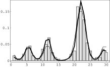
FIG. 1.: Reconstruction of an approximately periodic potential from coordinate measurements. (a) shows empirical density (bars), true likelihood (thin line), and reconstructed likelihood (thick line). (b) shows the true potential (thin line), reference potential $v_{0}$ = $\sin(\pi x/3)$ (dashed line), and reconstructed potential $v$ (thick line). (200 data points, mesh with 30 points, $m$ = 0.25, $\beta$ = 4, ${\bf K}_{0}$ = $-\Delta$, $\lambda$ = 0.2, $\mu$ = 0, $U(v_{\rm true})$ = $-0.354$ resulting in $U(v)$ = $-0.552$.)

   

FIG. 2.: Reconstruction with energy penalty term $E_{U}$ with $\kappa$ = $U(v_{\rm true})$ = $-0.354$. Shown are true potential (thin lines), reconstructed potential (thick lines), reference potential (dashed). (a) $K_{0}$ = $-\Delta$, $v_{0}(x)$ = $\sin(\pi x/3)$, $\mu$ = 1000, $U(v)$ = $-0.353$. (b) ${\bf K}_{0}$ = $-\Delta-\gamma\Delta_{T}$, $v_{0}\equiv 0$, $T$ = 6, $\gamma$ = 0.12, $\lambda$ = 0.05, $\mu$ = 10, $U(v)$ = $-0.351$. All other parameters as for Fig.1.

   

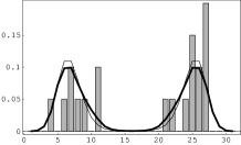
FIG. 3.: Reconstruction of symmetric potential with mixture of Gaussian priors. (a) shows empirical density (bars), true likelihood (thin line), and reconstructed likelihood (thick line). (b) shows the true potential (thick line), the two reference potential $v_{1}$ and $v_{2}$ (dashed lines), and the reconstructed potential $v$ (thick line). (20 data points, mesh with 31 points, for $v(x)$ = $v(-x)$ and boundary condition $v(\pm 15)$ = 0, with $m$ = 0.1, $\beta$ = 1, ${\bf K}_{0}$ = $-\Delta$, $\lambda$ = 0.5, $\mu$ = 10 $\kappa$ = $-9.66$ = $U(v_{\rm true})$ resulting in $U(v)$ = $-10.1$. ) Because both reference potentials are partially supported by the data the approximated $v$ is essentially a smoothed mixture between $v_{1}$ and $v_{2}$ in regions where no data are available with mixture coefficients for prior components $p_{0}(1|v)$ = 0.57, $p_{0}(2|v)$ = 0.43.

In the following numerical examples we discuss the reconstruction of an approximately periodic, one–dimensional potential. As a first example, assume we expect $v$ to be similar to a periodic reference potential $v_{0}$, which we choose as reference potential. To enforce the deviation from $v_{0}$ to be smooth we take as prior on $v$ a negative Laplacian covariance, i.e., ${\bf K}_{0}$ = $-\Delta$. Fig.1 shows representative numerical results for a grid with 30 points and 200 data sampled from a true likelihood $p(x|\hat{x},v_{\rm true})$ corresponding to a true potential $v_{\rm true}$. The reconstructed potential $v$ have been found by iterating without energy penalty term $E_{U}$ according to Eq.(18) with ${\bf A}$ = ${\bf K}_{0}$. Choosing zero boundary conditions for $v$ the matrix ${\bf K}_{0}$ is invertible. Consistent with the boundary conditions on $v$ we took periodic boundary conditions for the eigenfunctions $\phi_{\alpha}$. Note that the data have been sufficient to identify clearly the deviation from the periodic reference potential. Fig.2a shows the same example with an energy penalty term $E_{U}$ with $\kappa$ = $U(v_{\rm true})$. While the reconstructed likelihood (not shown) is not much altered, the true potential is now better approximated in regions where it is small.

Fig.2b shows the implementation of approximate periodicity by an operator $\Delta_{T}$ measuring the difference between the potential $v(x)$ and the potential translated by $T$ and and which is defined by $<\!\!v|\Delta_{T}|v\!\!>$ = $\int\!dx|v(x)-v(x+T)|^{2}$ for periodic boundary conditions on $v$. To find smooth solutions we added a negative Laplacian term with zero reference potential, i.e., we used ${\bf K}_{0}$ = $-\Delta-\gamma\Delta_{T}$. To have an invertible matrix for periodic boundary conditions on $v$ we iterated this time with ${\bf A}$ = ${\bf K}_{0}$ + $0.1{\bf I}$. The implementation of approximate periodicity by $\Delta_{T}$ instead of an periodic $v_{0}$ is more general in as far it allows arbitrary functions with period $T$. As, however, the reference function of the Laplacian term does not fit the true potential very well, the reconstruction is poorer in regions where the potential is large and thus no data are available. In these regions a priori information is of special importance. Finally, Fig.3 shows the implementation of a mixture of Gaussian prior processes.

In conclusion, we have applied a nonparametric Bayesian approach to inverse quantum statistics and shown its numerical feasibility for one–dimensional examples.

REFERENCES

- [1] A. Tikhonov and V. Arsenin, Solution of Ill–posed Problems (Wiley, New York, 1977).
- [2] V. Vapnik, Estimation of dependencies based on empirical data (Springer Verlag, New York, 1982).
- [3] A. Kirsch, An Introduction to the Mathematical Theory of Inverse Problems (Springer Verlag, New York, 1996).
- [4] R. Newton, Inverse Schrödinger Scattering in Three Dimensions (Springer Verlag, Berlin, 1989).
- [5] K. Chadan, D. Colton, L. Päivärinta, and W. Rundell, An Introduction to Inverse Scattering and Inverse Spectral Problem (SIAM, Philadelphia, 1997).
- [6] B. Zakhariev and V. Chabanov, Inverse Problems 13, R47 (1997).
- [7] G. Wahba, Spline Models for Observational Data (SIAM, Philadelphia, 1990).
- [8] J. Hertz, A. Krogh, and R. Palmer, Introduction to the Theory of Neural Computation, Vol. 1 of Lecture Notes Santa Fe Institute (Addison–Wesley, Redwood City, CA, 1991).
- [9] Machine Learning, Neural and Statistical Classification, edited by D. Michie, D. Spiegelhalter, and C. Taylor (Ellis Horwood, New York, 1994).
- [10] V. Vapnik, The Nature of Statistical Learning Theory (Springer Verlag, New York, 1995).
- [11] S. Lauritzen, Graphical Models (Oxford University Press, Oxford, 1996).
- [12] C. K. I. Williams and C. E. Rasmussen, in Advances in Neural Information Processing Systems, edited by D. S. Touretzky, M. C. Mozer, and M. E. Hasselmo (The MIT Press, Cambridge, MA, 1996), Vol. 8, pp. 514–520.
- [13] J. Berger, Statistical Decision Theory and Bayesian Analysis (Springer Verlag, New York, 1980).
- [14] C. Robert, The Bayesian Choice (Springer Verlag, New York, 1994).
- [15] A. Gelman, J. Carlin, H. Stern, and D. Rubin, Bayesian Data Analysis (Chapman & Hall, New York, 1995).
- [16] F. Girosi, M. Jones, and T. Poggio, Neural Computation 7, 219 (1995).
- [17] J. Lemm, in ICANN 99. Proceedings of the 9th International Conference on Artificial Neural Networks, Edinburgh, UK, 7–10 September 1999 (Springer Verlag, London, 1999).