Cahn-Hilliard theory for unstable granular flows

Abstract

A Cahn-Hilliard-type theory for hydrodynamic fluctuations is proposed that gives a quantitative description of the slowly evolving spatial correlations and structures in density and flow fields in the early stages of evolution of freely cooling granular fluids. Two mechanisms for pattern selection and structure formation are identified: unstable modes leading to density clustering (compare spinodal decomposition), and selective noise reduction (compare peneplanation in structural geology) leading to vortex structures. As time increases, the structure factor for the density field develops a maximum, which shifts to smaller wave numbers. This corresponds to an approximately diffusively growing length scale for density clusters. The spatial velocity correlations exhibit algebraic decay $\sim r^{-d}$ on intermediate length scales. The theoretical predictions for spatial correlation functions and structure factors agree well with molecular dynamics simulations of a system of inelastic hard disks.

I Introduction

Granular fluids in rapid flow stand out as an interesting and complex many-body problem, on which an impressive amount of experimental, simulation and theoretical results have been gathered in recent years. Advanced high speed measuring techniques, used in real experiments, as well as sophisticated visualization methods, used in computer experiments, have produced a lot of high quality data, which have led to intuitive and qualitative explanations. However, the experimental conditions are either too complex or the relevant physical parameters unknown to allow quantitative theoretical modeling and analysis.

On the other hand there exists a large body of analytic results obtained from hydrodynamic equations, from kinetic theory and from simplified mathematical models (on instabilities in flows, on clustering, on transport properties and non-Gaussian features in velocity distributions) that are not (yet) accessible to measurements in laboratory or computer experiments. There are a few notable exceptions, which will be discussed below in so far as they are relevant for the subject of the present paper.

Recently we have proposed a new mesoscopic theory, based on fluctuating hydrodynamics with unstable modes (Cahn-Hilliard-type theory) that provides detailed predictions on spatial correlation functions and structure factors, which permit a quantitative comparison with molecular dynamics (MD) simulations on fluids of inelastic hard spheres. Preliminary accounts of the results were published in Refs. [1, 2]. This paper [3] gives a comprehensive account of the underlying theoretical ideas, quantitative predictions and the detailed calculations. A subsequent paper [4] gives a comprehensive account of the quantitative comparisons with MD simulations, qualitative explanations where detailed theory is lacking, as well as discussions on ranges of validity and unresolved issues.

The inelasticity of the collisions between grains makes driven and undriven granular fluids behave very differently from atomic or molecular fluids. A dramatic difference with elastic fluids is that granular fluids lose kinetic energy through inelastic collisions and cool if energy is not supplied externally. In a thermodynamic sense, granular fluids should be considered as ‘open’ systems with an energy sink, created by the inelastic collisions. This collisional dissipation mechanism introduces several new time and length scales, which are often related to instabilities. In this paper we will focus on spatial correlation functions and structure factors, and on the underlying instabilities in freely evolving undriven granular fluids. There are two different mechanisms for pattern formation, one comparable to spinodal decomposition [5], a second one comparable to peneplanation in structural geology [6]. Moreover, we will discuss the importance of different intermediate scales, related to viscosity, heat conductivity and compressibility, which are controlled by the inelasticity.

The instabilities in undriven granular fluids have been studied by several authors [7, 8, 9, 10, 11, 12, 1, 2, 13, 14, 15]. Goldhirsch and Zanetti [7] were the first to perform molecular dynamics (MD) simulations of an undriven two-dimensional (2D) system of smooth inelastic hard disks and observed the spontaneous formation of density clusters. The system is unstable against spatial density fluctuations, so inhomogeneities in the density field (clusters) slowly grow to macroscopic size. However, before this happens, the granular fluid, prepared in a spatially homogeneous state, remains in a spatially homogeneous cooling state (HCS) with a slowly decreasing temperature. Gradually spatial inhomogeneities appear in the flow field (vortex patterns), and only much later density clusters are being observed. In Fig. 1 we show typical snapshots of the momentum field and the density field, as obtained in MD simulations of a system of inelastic hard disks [1, 2]. The flow field develops a large vorticity component and evolves into a ‘dense fluid of closely packed vortex structures’, which is still homogeneous on scales large compared to the average vortex diameter $L_{v}$, provided the systems are sufficiently large. More detailed information on the dynamics of clusters is available from very recent MD simulations [15].

The linear stability of undriven granular fluids was first analyzed by McNamara [9] on the basis of hydrodynamic equations for granular fluids. In Sec. II a detailed stability analysis is presented, which will be needed in analytic calculations of structure factors and correlation functions. The patterns that develop in the flow field correspond in fact to a relative instability: as momentum is conserved in collisions, perturbations in the flow field of large enough wavelength decay slower than the typical ‘thermal’ velocity, which decays as a result of the inelasticity of the collisions. In other words, as the system evolves, the noise from the thermal motion is reduced, which makes the initial long wavelength fluctuations in the flow field observable. However, their magnitude remains bounded by their values in the initial homogeneous state. In $d$-dimensional granular fluids, the modes corresponding to this relative instability are the $(d-1)$ transverse velocity or shear modes, as well as the long wavelength longitudinal velocity modes. In Secs. II and III we will show how the velocity fluctuations, at finite wave numbers, couple to density fluctuations, resulting in a linear instability of the density field. Unlike the flow field instability, the density instability is an absolute instability, giving rise to macroscopic clustering.

Comparison of Figs. 1 and 2 shows how the spatial inhomogeneities in density and flow field, slow down the cooling. Initially the system follows Haff’s cooling law [16], as will be briefly discussed in the next section. Once the inhomogeneities have become important, the homogeneous cooling law breaks down at a time $\tau_{c}$, estimated in Fig. 2 and in Ref. [14], and the system crosses over to the nonlinear clustering regime with a slower energy decay. This happens the more rapidly, the larger the inelasticity $\epsilon$. In Ref. [14], a mode coupling theory is described, which perturbatively takes the effect of the inhomogeneities on the energy decay into account and employs the decay of long wavelength fluctuations. This theory gives quantitative explanations of the energy decay observed in Fig. 2 at short and long times provided that the inelasticity ($\alpha\gtrsim 0.6$) and packing fraction ($\phi\lesssim 0.4$ in 2D) are not too large. A more general mode coupling theory is developed in Ref. [17].

In order to understand and quantify the patterns of Fig. 1, we study the time dependent spatial correlation functions of the corresponding fluctuations, using Landau and Lifshitz’s theory of fluctuating hydrodynamics [18], adapted to dissipative hard sphere fluids, i.e. adapted to the presence of unstable modes. We present a theory that describes the buildup of spatial correlations in the density and flow field in the initial regime, where the inhomogeneities are governed by linear hydrodynamics, i.e. linearized around the homogeneous cooling state (HCS). To motivate and explain the theory we compare a freely evolving granular fluid with spinodal decomposition [5], where the observed phenomena are similar in several respects.

In spinodal decomposition a mixture is prepared in a spatially homogeneous state (analogous to the homogeneous cooling state) by a deep temperature quench into the unstable region. In this region long wavelength composition fluctuations are unstable (analogous to density fluctuations in granular fluids) and lead to phase separation and pattern formation (analogous to the formation of density clusters and vortex patterns). This instability and the concomitant pattern formation are explained by the Cahn-Hilliard (CH) theory [5], where the time dependent structure factor for composition fluctuations, $S_{nn}(k,t)$, is calculated on the basis of a macroscopic diffusion equation. In the CH theory the unstable composition fluctuations are described by a $k$-dependent diffusion coefficient, which is negative below a certain threshold wave number.

The Cahn-Hilliard theory has also been used in the theory of two-dimensional turbulence (see Frisch [19] and references therein), where the behavior of the fluctuations in the flow field of incompressible fluids has been described in terms of negative eddy viscosities. Vorticity modes with negative effective viscosities have also been used by Rothman to study vortex formation in lattice gas cellular automata [20].

The instability of undriven granular fluids also differs in many details from spinodal decomposition. The former is a slow, the latter a fast process. Consequently, the Cahn-Hilliard theory in spinodal decomposition only describes the onset length and time scales of phase separation. As the formation of vortices and clusters in undriven granular fluids is a rather slow process, the present theory is expected to give a good description up to times which are rather large (see Figs. 1 and 2) on time scales that can be reached in molecular dynamics simulations, provided the inelasticity and the density are not too large.

The dynamics of fluctuations in granular fluids, say, in density, $\delta n({\bf r},t)=n({\bf r},t)-\langle n\rangle$, and flow field, ${\bf u}({\bf r},t)$, have hardly been studied [7, 12, 13], in sharp contrast to the average behavior, as witnessed by a large number of publications. We first recall that fluctuations are absent in standard hydrodynamic as well as in Boltzmann-Enskog-type kinetic equations which are based on molecular chaos (mean field assumption).

The objects of interest in this article are the equal-time spatial correlation functions of the fluctuating hydrodynamic fields $\delta a({\bf r},t)=a({\bf r},t)-\langle a\rangle$, where $a,b=\{n,T,u_{\alpha}\}$ with $\alpha=x,y,\dots$ denoting Cartesian components,

$$G_{ab}({\bf r},t)=V^{-1}\int{\rm d}{\bf r}^{\prime}\langle\delta a({\bf r}+{\bf r}^{\prime},t)\delta b({\bf r}^{\prime},t)\rangle.$$ (1)

The structure factors are the corresponding Fourier transforms,

$$S_{ab}({\bf k},t) = \int{\rm d}{\bf r}\exp(-i{\bf k}\cdot{\bf r})G_{ab}({\bf r},t)$$ (2)

$$= V^{-1}\langle\delta a({\bf k},t)\delta b(-{\bf k},t)\rangle,$$ (3)

where $\delta a({\bf k},t)$ is the Fourier transform of $\delta a({\bf r},t)$, and $V=L^{d}$ is the volume of the system. Goldhirsch et al. [7] initiated MD studies of $S_{nn}({\bf k},t)$ and $S_{pp}({\bf k},t)=\sum_{\alpha}S_{\alpha\alpha}({\bf k},t)$, and related in a qualitative way the structure at small $k$ to the most unstable shear modes. They presented a nonlinear analysis to explain the enslaving of density fluctuations by the vorticity field. This analysis reveals that the length scale associated with the late stages of nonlinear clustering is of the order $\xi_{\perp}\sim l_{0}/\sqrt{\epsilon}$, where $\epsilon=1-\alpha^{2}$ measures the inelasticity and $l_{0}$ is the mean free path. Brey et al. have also studied the nonlinear response of the density field to an initially excited ${\bf k}$ mode in the transverse flow field [21].

The most important function to describe the clustering instability is the structure factor $S_{nn}(k,t)$. A first step in its theoretical understanding has been given by Deltour and Barrat [12]. These authors have shown how its growth rate in the linear regime is determined by the most unstable long wavelength part of the heat mode, in which the density couples to longitudinal velocity perturbations.

The main goal of the present paper is to study the velocity and density correlation functions in undriven granular flows and to demonstrate the importance of internal fluctuations. In Secs. III and IV we discuss two different mechanisms for pattern formation, one leading to density clusters (spinodal decomposition), and one leading to vortex structures (peneplanation), and we we calculate the structure factors and show that a mesoscopic description in terms of fluctuating hydrodynamics [18] gives quantitative predictions for the spatial correlations functions over large intermediate time intervals, controlled by linearized hydrodynamics.

In Sec. V an analytic description of the correlation function $G_{\alpha\beta}({\bf r},t)$ of the components $u_{\alpha}({\bf r},t)$ of the flow field will be given, based on fluctuating hydrodynamics and the assumption of incompressible flow. This theory was presented in Ref. [1] and yields predictions, including long range tails $\sim r^{-d}$ in $d$-dimensional fluids, that for nearly elastic particles ($\alpha\gtrsim 0.9$) agree well with two-dimensional MD simulations up to large distances. As the transverse velocity fluctuations of an incompressible fluid do not couple to the density fluctuations in a linear theory, this theory gives no information on $S_{nn}(k,t)$. A quantitative theory for the magnitude of $S_{nn}(k,t)$ and its $k$ dependence in the full range of hydrodynamic wave numbers was given in Ref. [2] and is described in the second part of Sec. V, where the assumption of incompressibility is dropped and the description is extended to the general compressible case, based on the full set of fluctuating hydrodynamic equations. The results are also compared with computer simulations. We end with some conclusions in Sec. VI.

II Hydrodynamic stability

In the present section we discuss the macroscopic hydrodynamic equations for inelastic hard sphere (IHS) fluids. Fluctuations will be considered in the next section. We assume that IHS hydrodynamics for weakly inelastic systems can be described by the standard hydrodynamic conservation equations supplemented by a sink term $\Gamma$ in the temperature balance equation,

$$\partial_{t}n+\mbox{\boldmath$\nabla$}\cdot(n{\bf u})=0$$ (4)

$$\partial_{t}{\bf u}+{\bf u}\cdot\mbox{\boldmath$\nabla$}{\bf u}=-\frac{1}{\rho}\mbox{\boldmath$\nabla$}\cdot\mbox{\boldmath$\Pi$}$$ (5)

$$\partial_{t}T+{\bf u}\cdot\mbox{\boldmath$\nabla$}T=-\frac{2}{dn}(\mbox{\boldmath$\nabla$}\cdot{\bf J}+\mbox{\boldmath$\Pi$}:\mbox{\boldmath$\nabla$}{\bf u})-\Gamma.$$ (6)

Here $\rho=mn$, ${\bf u}$ the flow velocity, and $\textstyle{\frac{1}{2}}dnT$ the kinetic energy density in the local rest frame of the IHS fluid. The pressure tensor $\Pi_{\alpha\beta}=p\delta_{\alpha\beta}+\delta\Pi_{\alpha\beta}$ contains the local pressure $p$ and the dissipative momentum flux $\delta\Pi_{\alpha\beta}$, which is proportional to $\nabla_{\alpha}u_{\beta}$ and contains the kinematic and longitudinal viscosities $\nu$ and $\nu_{l}$, defined below Eq. (A3) of App. A. The constitutive relation for the heat flux, ${\bf J}=-\kappa\mbox{\boldmath$\nabla$}T$, defines the heat conductivity $\kappa$. The above equations can be justified to lowest order in the inelasticity $\epsilon=1-\alpha^{2}$ [22, 23], and will be used for weakly inelastic systems, where the pressure is assumed to be given by its value for elastic hard spheres, $p=nT[1+2b(n)]$ with $b(n)$ given below (A3) in App. A. Note that ${\cal O}(\epsilon)$ contributions are being neglected here, because the Enskog-Boltzmann equation for IHS fluids predicts $p=nT[1+(1+\alpha)b(n)]$. Similarly, the transport coefficients $\nu$, $\nu_{l}$, and $\kappa$ are assumed to be given by the Enskog theory for a dense gas of elastic hard spheres (EHS) or disks [24]. In the present paper, corrections of ${\cal O}(\epsilon)$ to the leading nonvanishing behavior of thermodynamic properties and transport fluxes will be neglected. More general expressions for transport coefficients have been derived in Refs. [25, 26, 27, 28, 29]. They contain an additional contribution, $-\mu\mbox{\boldmath$\nabla$}n$, in the heat flux, where the new transport coefficient $\mu\sim\epsilon$ vanishes for small inelasticity.

Kinetic theory provides an exact expression for the collisional dissipation rate $\Gamma$, which represents the average energy loss through inelastic collisions. It can be derived from the microscopic energy loss per collision. An explicit derivation can be found in Refs. [16, 25, 28]. For the present purpose however, a phenomenological derivation suffices, which proceeds as follows. On average, a particle loses per collision an amount $\sim\epsilon T$ of its kinetic energy, and per unit time an amount $\sim\epsilon\omega T$, where $\omega$ is the average collision frequency [24]. This argument gives (apart from a numerical factor $1/d$)

$$\Gamma=2\gamma_{0}\omega T,$$ (7)

where $\gamma_{0}=(1-\alpha^{2})/2d$. In the present theory the collision frequency is assumed to be given by Enskog’s theory for dense hard sphere fluids [24], and quoted explicitly in Eq. (A4) of App. A. It is proportional to $\sqrt{T}$.

For an understanding of what follows two properties of undriven granular fluids are important: (i) the existence of a homogeneous cooling state (HCS) and (ii) its linear instability against spatial fluctuations. We first observe that the hydrodynamic equations for an IHS fluid, initialized in a homogeneous state with temperature $T_{0}$, admit an HCS solution with a homogeneous density $n$, a flow field which can be set to zero everywhere, and a homogeneous temperature $T(t)$, determined by $\partial_{t}T=-\Gamma$. To solve this equation it is convenient to change to a new time variable, defined as ${\rm d}\tau=\omega(T(t)){\rm d}t$, yielding $T(t)=T_{0}\exp(-2\gamma_{0}\tau)$. To find the relation between the ‘internal’ time $\tau$, which measures the average number of collisions suffered per particle within a time $t$, and the ‘external’ time $t$, we integrate the relation for ${\rm d}\tau$ using $\omega\sim\sqrt{T}$, with the result

$$\tau=\frac{1}{\gamma_{0}}\ln[1+\gamma_{0}t/t_{0}].$$ (8)

In the elastic limit ($\epsilon\rightarrow 0$), it is proportional to the external time, $\tau=t/t_{0}$, measured in units of the mean free time $t_{0}=1/\omega(T_{0})$ at the initial temperature. The theoretical prediction (8) agrees well with the computer simulations [4] until the system crosses over at $\tau_{c}$ into the nonlinear clustering regime, to be discussed below. The initial slope of $\tau(t)$ corresponds to the collision frequency $\omega(T_{0})$ in the equilibrium state at $\tau=0$. The relation (8) introduces a new intermediate (mesoscopic) time scale, the homogeneous cooling time $t_{e}=t_{0}/\gamma_{0}$. Combination of these results yields the slow decay of the temperature,

$$T(t)=T_{0}\exp(-2\gamma_{0}\tau)=T_{0}/(1+\gamma_{0}t/t_{0})^{2},$$ (9)

which is Haff’s well-known homogeneous cooling law [16]. There exist extensive verifications of the validity of Haff’s law in the HCS ($\tau\ll\tau_{c}$ in Fig. 2) using MD simulations [8, 10, 12]. We show below that this HCS solution is linearly unstable once the linear extent $L$ of the system exceeds some dynamic correlation length $\sim l_{0}/\sqrt{\epsilon}$ [7, 9], where $l_{0}$ is the (time independent) mean free path. It is given by $l_{0}=v_{0}/\omega$, where $v_{0}=\sqrt{2T/m}$ is the thermal velocity.

In general the HCS is highly nontrivial, as it exhibits correlations between the velocities and positions of different particles. In the ‘lowest order’ description (for more refined approximations see [25, 28, 30]) the HCS corresponds to an equilibrium state, which is cooling adiabatically, i.e. with time dependent temperature (9). Here velocity correlations between different particles are absent, and position correlations are taken into account through the pair correlation function at contact (see (A4) of App. A).

In the present paper, we are interested in the buildup of correlations between spatial fluctuations in a system that is prepared in a homogeneous state at an initial temperature $T_{0}$. It reaches the HCS within a few mean free times $t_{0}$. Therefore, we can linearize Eqs. (6) around the homogeneous density $n$ and temperature $T(t)=T_{0}/[1+\gamma_{0}t/t_{0}]^{2}$, and the vanishing flow field of the slowly evolving HCS. The resulting set of linearized hydrodynamic equations, given in (A3) of App. A, contains the Enskog hard sphere transport coefficients, $\nu$, $\nu_{l}$ and $\kappa$, which are proportional to $\sqrt{T(t)}$, and depend therefore explicitly on time. It is again convenient to make the transformation ${\rm d}\tau=\omega{\rm d}t$, and introduce the dimensionless variables $\delta\tilde{n}({\bf r},\tau)=\delta n({\bf r},t)/n$, $\tilde{\bf u}({\bf r},\tau)={\bf u}({\bf r},t)/v_{0}(t)$, and $\delta\widetilde{T}({\bf r},\tau)=\delta T({\bf r},t)/T(t)$. In these new variables the equations of change for the macroscopic Fourier modes $\delta\tilde{n}({\bf k},\tau)$, $\tilde{\bf u}({\bf k},\tau)$, and $\delta\widetilde{T}({\bf k},\tau)$, defined through $\delta\tilde{a}({\bf k},\tau)=\int{\rm d}{\bf r}\exp(-i{\bf k}\cdot{\bf r})\delta\tilde{a}({\bf r},\tau)$, become ordinary differential equations with time independent coefficients (valid for $kl_{0}\lesssim 1$), which can be analyzed in terms of eigenvalues and eigenvectors,

$$\frac{\partial\delta\tilde{n}}{\partial\tau} = -ikl_{0}\tilde{u}_{l}$$ (10)

$$\frac{\partial\tilde{u}_{\perp}}{\partial\tau} = \gamma_{0}(1-k^{2}\xi_{\perp}^{2})\tilde{u}_{\perp}$$ (11)

$$\frac{\partial\tilde{u}_{l}}{\partial\tau} = \gamma_{0}(1-k^{2}\xi_{l}^{2})\tilde{u}_{l}-ikl_{0}\left(\frac{p}{2nT}\right)\delta\widetilde{T}$$ (13)

$$-ikl_{0}\left(\frac{1}{2nT\chi_{T}}\right)\delta\tilde{n}$$

$$\frac{\partial\delta\widetilde{T}}{\partial\tau} = -\gamma_{0}(1+k^{2}\xi_{T}^{2})\delta\widetilde{T}-ikl_{0}\left(\frac{2p}{dnT}\right)\tilde{u}_{l}$$ (15)

$$-\gamma_{0}g(n)\delta\tilde{n}.$$

Here we have introduced the time independent correlation lengths $\xi_{\perp}$, $\xi_{l}$ and $\xi_{T}$, defined by $\xi_{\perp}^{2}=\nu/\omega\gamma_{0}$, $\xi_{l}^{2}=\nu_{l}/\omega\gamma_{0}$ and $\xi_{T}^{2}=2\kappa/dn\omega\gamma_{0}$, the isothermal compressibility $\chi_{T}={(\partial n/\partial p)}_{T}/n$, and for the function $g(n)=2[1+(n/\chi)\partial\chi/\partial n]$ we refer to Eqs. (A3) and (A4) of App. A. The subscript $\perp$ in the equation for $\tilde{u}_{\perp}$ refers to any of the $(d-1)$ directions perpendicular to ${\bf k}$, and the subscript $l$ denotes the longitudinal direction along ${\bf k}$. The validity of the hydrodynamic Eqs. (15) is restricted to wave numbers $k\ll 2\pi/l_{0}$ to guarantee separation of kinetic and hydrodynamic scales, and to $k\ll 2\pi/\sigma$, where $\sigma$ is the diameter of a disk or sphere, to guarantee that the Euler equations involve only local hydrodynamics. Therefore, the validity of the hydrodynamic Eqs. (15) are restricted to long wavelengths, satisfying $k\ll{\rm min}\{2\pi/l_{0},2\pi/\sigma\}$. In matrix representation we write the above equations as

$$\frac{\partial}{\partial\tau}\delta\tilde{\bf a}({\bf k},\tau)=\widetilde{\bf M}({\bf k})\delta\tilde{\bf a}({\bf k},\tau),$$ (16)

where components of $\tilde{\bf a}$ are labeled with $\{n,T,l,\perp\}$, and the hydrodynamic matrix $\widetilde{\bf M}$ is defined by Eqs. (15). The linear stability of (16) was first investigated in Refs. [7, 9]. Its eigenvalues or dispersion relations $\zeta_{\lambda}(k)$ and corresponding eigenvectors are analyzed in App. A. The $\zeta_{\lambda}(k)$ were first calculated numerically in Ref. [9], using transport coefficients somewhat different from those obtained from the Enskog theory. Typical results of our calculations are shown in Fig. 3. The most striking feature is that there are two eigenvalues, $\zeta_{\perp}$ and $\zeta_{H}$, that are positive below the threshold values $k_{\perp}^{\ast}$ and $k_{H}^{\ast}$, i.e. two linearly unstable modes with exponential growth rates. The spectrum has different characteristics for smaller and larger wavelengths. In the dissipative range [9] ($kl_{0}\ll\gamma_{0}$) all eigenvalues are real; propagating modes are absent. Around $kl_{0}\sim{\cal O}(\gamma_{0})$, two eigenvalues become complex conjugates and the corresponding (sound) modes become propagating. In the standard range ($kl_{0}\gg\gamma_{0}$), compression effects and sound propagation, which are ${\cal O}(kl_{0})$, dominate dissipation, whereas heat conduction, which is ${\cal O}(k^{2}l_{0}^{2})$, becomes dominant only in the elastic range ($kl_{0}\gg\sqrt{\gamma_{0}}$), where $\gamma_{0}$ is assumed to be sufficiently small so that $\gamma_{0}\ll\sqrt{\gamma_{0}}$. In the latter range, the dispersion relations and eigenmodes resemble those of an elastic fluid. In App. A the full set of eigenvalues $\zeta_{\lambda}(k)$ and eigenmodes is analyzed. Here we only analyze the $(d-1)$-fold degenerate transverse velocity or shear modes, which are decoupled from the remaining modes. In fact, Eqs. (15) show already that $\zeta_{\perp}(k)=\gamma_{0}(1-k^{2}\xi_{\perp}^{2})$, which describes an unstable mode for $k<k_{\perp}^{\ast}=1/\xi_{\perp}$.

Similarly, the heat mode is unstable for $k<k_{H}^{\ast}\propto 1/\xi_{T}$, as shown in App. A. In the dissipative range ($kl_{0}\ll\gamma_{0}$), the heat mode is given by $\zeta_{H}(k)=\gamma_{0}(1-k^{2}\xi_{\parallel}^{2})$ where $\xi_{\parallel}$ is calculated in App. A. In this range the heat mode is a pure longitudinal velocity fluctuation. We point out that $\xi_{\perp}$ diverges as $1/\sqrt{\epsilon}$ for small $\epsilon$, while $\xi_{\parallel}\sim 1/\epsilon$ [see (A14)]. As a consequence the correlation lengths $\xi_{\perp}$ and $\xi_{\parallel}$ are well separated for small inelasticity, as shown in Fig. 4.

Furthermore, we observe that the instability of shear and heat mode is a long wavelength instability. As a consequence, for finite systems effects of the boundaries are important, and the various instabilities are suppressed in small systems. When using periodic boundary conditions, the instabilities are suppressed if $k_{\rm min}=2\pi/L$ is larger than $k_{\perp}^{\ast}$ or $k_{H}^{\ast}$. When decreasing the system length $L=V^{1/d}$ at fixed inelasticity, first the heat mode will become stable ($k_{H}^{\ast}<k_{\rm min}<k_{\perp}^{\ast}$). In this range the density (coupled to the heat mode) is linearly stable, and density inhomogeneities can only be created via a nonlinear coupling to the unstable shear mode [7]. Decreasing the system size even further ($k_{\perp}^{\ast}<k_{\rm min}$) will stabilize the shear mode and thus the HCS itself. In the next section we present a mesoscopic theory to describe the dynamics of the long wavelength fluctuations in the system.

III Mesoscopic hydrodynamics

In this section we study spatial fluctuations, around a reference state, of the hydrodynamic fields, which leads to a Cahn-Hilliard-type theory [5] for the structure factors. The dynamics of these fluctuations can be described by the fluctuating hydrodynamic equations [18], obtained from the nonlinear equations (6) by adding fluctuation terms to the momentum and heat current, denoted by $\hat{\mbox{\boldmath$\Pi$}}$ and $\hat{\bf J}$ respectively. These currents $\hat{\mbox{\boldmath$\Pi$}}$ and $\hat{\bf J}$ are considered as Gaussian white noise, local in space, and their correlations are determined by some appropriately formulated fluctuation-dissipation theorem for the reference state.

In elastic fluids the reference state would be the thermal equilibrium state. In driven systems it would be a nonequilibrium steady state (NESS). In the present case the reference state is the slowly evolving homogeneous cooling state. In lowest approximation [28] it may be considered as an adiabatically changing equilibrium state with a constant density, a vanishing flow field and a time dependent temperature, described by Haff’s law (9). The basic extension required for application to IHS fluids, is the assumption that the fluctuation-dissipation theorem also applies to the HCS with an adiabatically changing temperature $T(t)$. This assumption relates the noise strengths to the transport coefficients through [18]

$$\langle\hat{\Pi}_{\alpha\beta}({\bf r},t)\hat{\Pi}_{\gamma\delta}({\bf r}^{\prime},t^{\prime})\rangle=2T[\eta(\delta_{\alpha\gamma}\delta_{\beta\delta}+\delta_{\alpha\delta}\delta_{\beta\gamma})$$ (17)

$$\;\;\;\;\;\;\;\;\;\;\;\;\;\;\;\;\;\;+(\zeta-\frac{2}{d}\eta)\delta_{\alpha\beta}\delta_{\gamma\delta}]\delta({\bf r}-{\bf r}^{\prime})\delta(t-t^{\prime})$$ (18)

$$\langle\hat{J}_{\alpha}({\bf r},t)\hat{J}_{\beta}({\bf r}^{\prime},t^{\prime})\rangle=2\kappa T^{2}\delta_{\alpha\beta}\delta({\bf r}-{\bf r}^{\prime})\delta(t-t^{\prime}).$$ (19)

For dimensional reasons, the transport coefficients in systems with hard sphere type interactions, like IHS, are proportional to $\sqrt{T(t)}$.

In the present theory for nearly elastic fluids we linearize the nonlinear Langevin equations, obtained from (6), around the HCS. By applying the transformations introduced above Eqs. (15) we obtain the dynamic equations for the rescaled variables, in the form of a set of Langevin equations with constant coefficients $\widetilde{\bf M}({\bf k})$, i.e.

$$\frac{\partial}{\partial\tau}\delta\tilde{\bf a}({\bf k},\tau)=\widetilde{\bf M}({\bf k})\delta\tilde{\bf a}({\bf k},\tau)+\hat{\bf f}({\bf k},\tau),$$ (20)

where $\hat{\bf f}$ represents the rescaled internal fluctuations in the momentum and heat flux.

The equation of motion for the matrix of rescaled structure factors, $\tilde{S}_{ab}({\bf k},\tau)=V^{-1}\langle\delta\tilde{a}({\bf k},\tau)\delta\tilde{b}(-{\bf k},\tau)\rangle$, can now be derived from Eq. (20), and yields

$$\frac{\partial}{\partial\tau}\tilde{\bf S}({\bf k},\tau)=\widetilde{\bf M}({\bf k})\cdot\tilde{\bf S}({\bf k},\tau)+\tilde{\bf S}({\bf k},\tau)\cdot\widetilde{\bf M}^{T}(-{\bf k})+\tilde{\bf C}(k),$$ (21)

where $\widetilde{\bf M}^{T}$ is the transpose of $\widetilde{\bf M}$. It is to be solved for given initial values $\tilde{\bf S}({\bf k},0)$. In terms of the rescaled variables the Gaussian white noise (19) has the standard from with constant coefficients, given by the covariance matrix, $\tilde{\bf C}(k)$, with

$$V^{-1}\langle\hat{f}_{a}({\bf k},\tau)\hat{f}_{b}(-{\bf k},\tau^{\prime})\rangle=\tilde{C}_{ab}(k)\delta(\tau-\tau^{\prime}).$$ (22)

It is diagonal with nonvanishing elements

$$\tilde{C}_{TT} = 4\gamma_{0}k^{2}\xi_{T}^{2}/dn$$ (23)

$$\tilde{C}_{ll} = \gamma_{0}k^{2}\xi_{l}^{2}/n$$ (24)

$$\tilde{C}_{\perp\perp} = \gamma_{0}k^{2}\xi_{\perp}^{2}/n,$$ (25)

as follows from (19) and the definitions of the correlation lengths below (15). The formal solution of (21) for the matrix of rescaled structure factors is then

$$\tilde{\bf S}({\bf k},\tau)= \exp[\widetilde{\bf M}({\bf k})\tau]\cdot\tilde{\bf S}({\bf k},0)\cdot\exp[\widetilde{\bf M}^{T}(-{\bf k})\tau]$$ (26)

$$+\int_{0}^{\tau}{\rm d}\tau^{\prime} \exp[\widetilde{\bf M}({\bf k})\tau^{\prime}]\cdot\tilde{\bf C}(k)\cdot\exp[\widetilde{\bf M}^{T}(-{\bf k})\tau^{\prime}].$$ (27)

At the initial time ($\tau=0$) the system is prepared in a thermal equilibrium state of elastic hard spheres with density $n$ and temperature $T_{0}$. Consequently, all elements of $\tilde{\bf S}({\bf k},0)$ are known. Moreover, the evolution equations (21) and (15) are only valid for $k\ll\{2\pi/l_{0},2\pi/\sigma\}$. So the initial values $\tilde{\bf S}({\bf k},0)$ are only needed for $k\sigma\ll 2\pi$, where they are given by their limiting values as $k\rightarrow 0$. The nonvanishing $\tilde{S}_{ab}({\bf k},0)$ with $a,b=\{n,T,l,\perp\}$ are given by their equipartition values for elastic hard sphere fluids,

$$\tilde{S}_{nn}(k,0) = T\chi_{T}$$ (28)

$$\tilde{S}_{TT}(k,0) = \frac{2}{dn}$$ (29)

$$\tilde{S}_{ll}(k,0) = \tilde{S}_{\perp\perp}(k,0)=\frac{1}{2n}.$$ (30)

The above equations can be solved numerically or analytically. For a theoretical analysis it is more convenient to study the deviations from the initial values in thermal equilibrium, defined as

$$\tilde{\bf S}^{+}({\bf k},\tau)=\tilde{\bf S}({\bf k},\tau)-\tilde{\bf S}({\bf k},0).$$ (31)

The reason is that $\tilde{\bf S}({\bf k},\tau)$ itself at larger $k$ values also approaches $\tilde{\bf S}({\bf k},0)$ by the imposed fluctuation-dissipation theorem (19) or (22). Inspection of (21) for $kl_{0}\gg\sqrt{\gamma_{0}}$ (elastic range) shows that all $k$ independent terms in the matrix $\widetilde{\bf M}({\bf k})$ in (15) can be neglected and the hydrodynamic matrix reduces to the elastic one, $\tilde{\bf E}({\bf k})$. Consequently, Eq. (21) reduces to

$$\tilde{\bf E}({\bf k})\cdot\tilde{\bf S}({\bf k},0)+\tilde{\bf S}({\bf k},0)\cdot\tilde{\bf E}^{T}(-{\bf k})+\tilde{\bf C}(k)={\bf 0},$$ (32)

as can be verified using (25) and (30).

Subtracting this equation from (21) yields an equation of a similar form as (21),

$$\frac{\partial}{\partial\tau}\tilde{\bf S}^{+}({\bf k},\tau) = \widetilde{\bf M}({\bf k})\cdot\tilde{\bf S}^{+}({\bf k},\tau)$$ (33)

$$+ \tilde{\bf S}^{+}({\bf k},\tau)\cdot\widetilde{\bf M}^{T}(-{\bf k})+\tilde{\bf B}(k),$$ (34)

with a source term

$$\tilde{\bf B}(k) = [\widetilde{\bf M}({\bf k})-\tilde{\bf E}({\bf k})]\cdot\tilde{\bf S}({\bf k},0)$$ (35)

$$+ \tilde{\bf S}({\bf k},0)\cdot[\widetilde{\bf M}^{T}(-{\bf k})-\tilde{\bf E}^{T}(-{\bf k})].$$ (36)

Its nonvanishing matrix elements are

$$\tilde{B}_{nT} = \tilde{B}_{Tn}=-\gamma_{0}g(n)\tilde{S}_{nn}(k,0)$$ (37)

$$\tilde{B}_{TT} = -2\gamma_{0}\tilde{S}_{TT}(k,0)$$ (38)

$$\tilde{B}_{ll} = 2\gamma_{0}\tilde{S}_{ll}(k,0)$$ (39)

$$\tilde{B}_{\perp\perp} = 2\gamma_{0}\tilde{S}_{\perp\perp}(k,0),$$ (40)

and the formal solution of (34) with the initial value $\tilde{\bf S}^{+}({\bf k},0)=0$ becomes,

$$\tilde{\bf S}^{+}({\bf k},\tau)=\int_{0}^{\tau}{\rm d}\tau^{\prime}\exp[\widetilde{\bf M}({\bf k})\tau^{\prime}]\cdot\tilde{\bf B}(k)\cdot\exp[\widetilde{\bf M}^{T}(-{\bf k})\tau^{\prime}].$$ (41)

The spectral decomposition (A9) of App. A allows us to write the rescaled structure factors for $a,b=\{n,T,l,\perp\}$ as

$$\tilde{S}^{+}_{ab}({\bf k},\tau) = \sum_{\lambda\mu}\tilde{w}_{\lambda a}({\bf k})\tilde{w}_{\mu b}(-{\bf k})\tilde{\cal B}_{\lambda\mu}(k)\times$$ (43)

$$\left(\frac{\exp[(\zeta_{\lambda}+\zeta_{\mu})\tau]-1}{\zeta_{\lambda}+\zeta_{\mu}}\right)$$

where we have introduced

$$\tilde{\cal B}_{\lambda\mu}(k)=\langle\tilde{\bf v}_{\lambda}({\bf k})|\tilde{\bf B}(k)|\tilde{\bf v}_{\mu}(-{\bf k})\rangle,$$ (44)

and the eigenvalues $\zeta_{\lambda}(k)$ depend only on $|{\bf k}|$ (see App. A). The results (27) or (43) yield the structure factors, which can be calculated numerically or analytically. Expression (27) is most convenient for numerical computation, whereas (43) is more suitable for our theoretical analysis in the long wavelength range. The expressions above contain exponentially growing factors describing the unstable modes, as in the Cahn-Hilliard (CH) theory, discussed in the introduction. The present theory includes in (27) the rapid microscopic fluctuations, induced by the Langevin noise $\tilde{\bf C}(k)$, and is equivalent to the Cahn-Hilliard-Cook theory [5]. If the Langevin noise is neglected by setting $\tilde{\bf C}(k)={\bf 0}$ in (27), we obtain the predictions of the noiseless CH theory,

$$\tilde{\bf S}({\bf k},\tau)=\exp[\widetilde{\bf M}({\bf k})\tau]\cdot\tilde{\bf S}({\bf k},0)\cdot\exp[\widetilde{\bf M}^{T}(-{\bf k})\tau].$$ (45)

or in component form

$$\tilde{S}_{ab}({\bf k},\tau)=\sum_{\lambda\mu}\tilde{w}_{\lambda a}({\bf k})\tilde{w}_{\mu b}(-{\bf k})\tilde{\cal S}_{\lambda\mu}({\bf k})\exp[(\zeta_{\lambda}+\zeta_{\mu})\tau],$$ (46)

where $\tilde{\cal S}_{\lambda\mu}({\bf k})$ is defined by (44) with $\tilde{\bf B}(k)$ replaced by $\tilde{\bf S}({\bf k},0)$.

The explicit solutions can be studied using the eigenvalues and eigenfunctions in different ranges of wave numbers. For the very long wavelengths in the dissipative range ($kl_{0}\ll\gamma_{0}=\epsilon/2d$) this will be done in the next section by $k$-expansion at fixed $\epsilon$. In general, the dissipative range ($kl_{0}\ll\gamma_{0}$) and the standard range ($kl_{0}\gg\gamma_{0}$) are accessible to analysis by rescaling the wavelengths as $k=\epsilon^{2}\tilde{k}$ or $k=\sqrt{\epsilon}\tilde{k}$ respectively, and taking the small-$\epsilon$ limit subsequently [9].

A theoretical analysis of the formal results, derived in this section, will be presented in Sec. IV. Before concluding this section we present the numerical results of (27) and (45) respectively with and without Langevin noise, where the relevant equations have been solved with Mathematica. The values of $S_{ab}({\bf k},t)$ ‘with noise’ are plotted as solid lines in Figs. 5, 6, and 7 for different components $(ab)$; the values ‘without noise’ are shown as dashed lines in Figs. 5(a) and 6.

The qualitative features of both theories are about the same, except that the large-$k$ limit of the results of (45) ‘without noise’ at fixed $t$ does not approach the plateau values (30), but vanishes. In the long wavelength and large time limit the results of both theories approach each other, but at finite $k$ there are substantial differences. It should of course be kept in mind that the Cahn-Hilliard theory without noise was only designed to explain the structure and instabilities on the largest wavelengths.

It is also of interest to observe that the locations of the maxima of $S_{nn}$ in Fig. 5 and those of the minima (‘dip’) of $S_{\parallel}$ in Fig. 6 approximately coincide. It indicates that the density instability is closely connected to the dynamics controlling $S_{\parallel}$. This turns out to be the heat mode, as we will show in the next section. The negative value of $\tilde{S}_{nT}(k,\tau)$ in Fig. 7 shows that density and temperature fluctuations are anticorrelated at all wavelengths.

An illustration of the comparison with the MD simulations on systems of inelastic hard disks of Refs. [1, 2, 4] is shown in Fig. 5(b) for $S_{nn}$ and in Fig. 6(b) for $S_{\perp}\equiv S_{\perp\perp}$ and $S_{\parallel}\equiv S_{ll}$. The agreement between theory and simulations is in general very good, even down to rather large inelasticities ($\alpha\gtrsim 0.6$). By comparing the simulation results for $S_{\perp}$ and $S_{\parallel}$ in Fig. 6(b) with the numerical results of our theory with noise (solid lines) and without (dashed lines), we have observed that the agreement in the former case extends over the full range of $k$ values, whereas in the latter case it is restricted to the small-$k$ range. Similar conclusions hold when comparing the simulation results for $S_{nn}(k,t)$ in Fig. 5(b) with the numerical results in Fig. 5(a) with and without Langevin noise included. A more comprehensive comparison with MD simulations for different densities and different inelasticities will be given in Ref. [4], where also the range of validity of the present theory will be explored.

IV Development of structure and instabilities

An elastic fluid in thermal equilibrium does not show any structure on hydrodynamic length scales ($k\lesssim{\rm min}\{1/l_{0},1/\sigma\})$. This means that the hydrodynamic structure factors $S_{ab}(k)$ are totally flat, independent of $k$, as can be seen in (30). The corresponding hydrodynamic correlation functions are short ranged, $G_{ab}({\bf r},t)\sim\delta({\bf r})$, on these length scales. Development of structure on length scales above the microscopic scales $\{l_{0},\sigma\}$ will manifest itself in the appearance of one or more maxima or peaks in the structure factors. A linear instability will manifest itself in a structure factor that grows exponentially in time. With these concepts in mind, we analyze the structure factors in (27) for the IHS fluid, as we want to determine which physical excitations are responsible for the features observed in the MD simulations and in the numerical solutions.

A Structures in the velocity field

We first consider the simplest case of the the transverse structure factor $S_{\perp}(k,t)=v_{0}^{2}(t)\tilde{S}_{\perp}(k,\tau)$ with $(ab)=(\perp\perp)$. It describes the transverse velocity or vorticity fluctuations $\tilde{u}_{\perp}({\bf k},\tau)$, which are decoupled in (15) from the remaining Fourier modes, and satisfy a one-component Langevin equation, where the matrix $\widetilde{\bf M}({\bf k})$ in (20) reduces to a single number $\zeta_{\perp}(k)=\gamma_{0}(1-\xi_{\perp}^{2}k^{2})$. The structure factor is readily found from (43) and yields

$$S_{\perp}^{+}(k,t) = v_{0}^{2}(t)\int_{0}^{\tau}{\rm d}\tau^{\prime}\tilde{B}_{\perp\perp}(k)\exp[2\zeta_{\perp}(k)\tau^{\prime}]$$ (47)

$$= \frac{T(t)}{mn}\left(\frac{\exp[2\gamma_{0}(1-\xi_{\perp}^{2}k^{2})\tau]-1}{1-\xi_{\perp}^{2}k^{2}}\right),$$ (48)

where $\textstyle{\frac{1}{2}}mv_{0}^{2}(t)=T(t)=T_{0}\exp(-2\gamma_{0}\tau)$. Combination of (31) and (48) yields the complete structure factor, $S_{\perp}(k,t)=v_{0}^{2}(t)[\tilde{S}_{\perp}(k,0)+\tilde{S}^{+}_{\perp}(k,\tau)]$, which is plotted as the upper solid line in Fig. 6(b). It does not grow, but slowly decays as $S_{\perp}(k,t)\simeq(T_{0}/mn)\exp(-2\gamma_{0}\xi_{\perp}^{2}k^{2}\tau)$ at the largest wavelengths. It simply represents vorticity diffusion on the ‘internal’ time scale $\tau$, with a diffusivity $\gamma_{0}\xi_{\perp}^{2}=\nu/\omega$, where the typical length scales of vortices grow [31] like $L_{v}(t)\sim 2\pi\xi_{\perp}\sqrt{2\gamma_{0}\tau}\sim 2\pi\sqrt{\nu\tau/\omega}$, which is independent of the degree of inelasticity.

Consider the noiseless CH theory in (45), which yields directly $S_{\perp}(k,t)=(T_{0}/mn)\exp(-2\gamma_{0}\xi_{\perp}^{2}k^{2}\tau)$ [upper dashed line in Fig. 6(b)]. It agrees with the full theory (48) [upper solid line in Fig. 6(b)] only in the small-$k$ limit, where the denominator $(1-\xi_{\perp}^{2}k^{2})$ in (48) can be replaced by 1. At finite $k$, the differences between both theories are relatively large. Moreover, the upper dashed line in Fig. 6(b) convincingly shows that the noiseless CH theory does not agree with the simulation results.

Next, we consider the longitudinal structure factor $S_{\parallel}(k,t)$ with $(ab)=(ll)$. As subsequent analysis will show, it is determined — in an almost quantitative manner — by a single mode, the heat mode. The fastest growing term in (43) is $(\lambda\mu)=(HH)$, as can be seen from Fig. 3. This leads in the structure factor $S_{\parallel}(k,t)=v_{0}^{2}(t)\tilde{S}_{\parallel}(k,\tau)$ to a slowly decaying contribution. All remaining contributions decay at least as fast as $v_{0}(t)\sim\exp(-\gamma_{0}\tau)$. The slowest decay occurs at very long wavelengths, i.e. in the dissipative range ($kl_{0}\ll\gamma_{0}$). The relevant coefficient $\tilde{\cal B}_{HH}(k)$ follows from (44), (40) and (A13) in App. A, and is given by

$$\tilde{\cal B}_{HH}(k) = \sum_{ab}\tilde{v}_{Ha}({\bf k})\tilde{v}_{Hb}(-{\bf k})\tilde{B}_{ab}(k)$$ (49)

$$= 2\gamma_{0}\tilde{S}_{ll}(k,0)=\frac{\gamma_{0}}{n}.$$ (50)

The required component of the right eigenvector, given in (A13), is $\tilde{w}_{Hl}({\bf k})\simeq 1$. Inserting these data in (43) and combining it with (31) yields for $kl_{0}\ll\gamma_{0}$,

$$S_{\parallel}(k,t)=\frac{T(t)}{mn}\left(1+\frac{\exp[2\gamma_{0}(1-\xi_{\parallel}^{2}k^{2})\tau]-1}{1-\xi_{\parallel}^{2}k^{2}}\right),$$ (51)

where the dispersion relation $\zeta_{H}(k)=\gamma_{0}(1-\xi_{\parallel}^{2}k^{2})$ has been used. This long wavelength approximation for $S_{\parallel}$ has the same form as the exact result (48) with $\xi_{\perp}$ replaced by $\xi_{\parallel}$. In Fig. 6(a) we compare the result (51) (dot-dashed lines) with the numerical solution (solid lines), presented in Sec. III. The simple analytic small-$k$ approximation (51) captures the global features at small $k$ and the plateaux at larger $k$ values quantitatively, but is missing the little dip at intermediate $k$ values.

The behavior of the longitudinal structure factor on the largest length scales follows again from Eqs. (51) as $S_{\parallel}(k,t)\simeq(T_{0}/mn)\exp(-2\gamma_{0}\xi_{\parallel}^{2}k^{2}\tau)$. This implies that the heat mode on the largest length scales is a purely diffusive mode with a diffusivity $\gamma_{0}\xi_{\parallel}^{2}$, which is much larger than the diffusivity $\gamma_{0}\xi_{\perp}^{2}$ for the vorticity (see Fig. 4), and the associated length scale grows like $L_{\parallel}(t)\sim 2\pi\xi_{\parallel}\sqrt{2\gamma_{0}\tau}$. Inspection of the eigenmodes $\{\tilde{\bf w}_{H}({\bf k}),\tilde{\bf v}_{H}({\bf k})\}$ in (A13) of App. A for $k\rightarrow 0$ shows that this diffusive mode is a pure longitudinal velocity field $\tilde{u}_{l}({\bf k},\tau)$. Its diffusivity $\gamma_{0}\xi_{\parallel}^{2}$, given in (A14) of App. A, depends for small inelasticities ($\gamma_{0}\rightarrow 0$) mainly on thermodynamic variables, like compressibility and pressure, and only slightly on transport coefficients.

The physical implications of Fig. 6 are quite interesting. It shows the phenomenon of noise reduction [14] at small wavelengths. With increasing time the noise strengths $S_{\parallel}(k,t)$ and $S_{\perp}(k,t)$ of the fluctuations in the flow field decrease at larger $k$ values and remain bounded for all $k$ and $t$ by their initial equipartition value $T_{0}/mn$, which is independent of $k$. This can be rephrased by stating that the flow field exhibits only a ‘relative’ instability.

The noise reduction is a direct consequence of the microscopic inelastic collision rule, which forces the particles to move more and more parallel in successive collisions. It is this ‘physical coarse graining’ process that selectively suppresses the shorter wavelength fluctuations in the flow field in an ever-increasing range of wavelengths. Consistent with this picture is also the selective suppression of the divergence of the flow field $u_{\parallel}({\bf k},t)$, which decays at a much faster rate $\gamma_{0}\xi_{\parallel}^{2}k^{2}$ than its rotational part $u_{\perp}({\bf k},t)$ that decays with a rate $\gamma_{0}\xi_{\perp}^{2}k^{2}$.

So, noise reduction is the pattern selection mechanism, responsible for the growing vortex structures observed in Fig. 1. An interesting analog from structural geology of the peak formed at ${\bf k}={\bf 0}$ in reciprocal space, is the formation of Ayers Rock (Mount Uluru) in the center of Australia, as a result of peneplanation by selective erosion [6].

B Unstable density structures

So far, we have seen that the velocity structure factors, $S_{\perp}(k,t)$ and $S_{\parallel}(k,t)$, develop structure, but remain bounded by their initial values. Next we will focus on the unstable structure factor $S_{nn}(k,t)$, which describes the density clustering in undriven IHS fluids. In the comparable case of spinodal decomposition the phase separation is driven by a single unstable mode, the composition fluctuations, described by the macroscopic equation $\partial_{t}\delta n({\bf k},\tau)=z_{D}(k)\delta n({\bf k},t)$, where the growth rate has the typical form $z_{D}(k)=\Delta k^{2}(1-\textstyle{\frac{1}{2}}\xi_{D}^{2}k^{2})$. The corresponding structure factor (45) in the noiseless Cahn-Hilliard theory has the form $S_{nn}(k,t)\sim\exp[2z_{D}(k)t]$, and exhibits a maximum growth rate at $k_{\rm max}=1/\xi_{D}$, where $z_{D}(k)$ has a maximum. This time independent length scale fails to describe the growing length scales of the patterns observed in spinodal decomposition [5].

However, the present theory does explain the growing correlation length $L_{\rm cl}(t)$ for the clusters in undriven IHS fluids in the early stages of cluster formation, as the numerical results for $S_{nn}(k,t)$ in Fig. 5 demonstrate. Its maximum at $k_{\rm max}(t)$ shifts to smaller $k$ values.

We first consider a naive version of the noiseless Cahn-Hilliard theory, proposed by Deltour and Barrat [12]. These authors assume that the structure factor $S_{nn}$ can be described by the unstable density field, i.e. $S_{nn}(k,t)\simeq S_{nn}(k,0)\exp[2\zeta_{H}(k)\tau]$, with the growth rate $\zeta_{H}(k)$ of the unstable heat mode. As $\zeta_{H}(k)$ decreases monotonically with $k$, as shown in Fig. 3, this structure factor shows the fastest growth at the smallest wave number $k_{\rm min}=2\pi/L$, allowed in a box of length $L$, and does not explain the dynamics of cluster growth.

Next we consider the full theory of Sec. III with Langevin noise included. Then the structure factor $S^{+}_{nn}(k,t)=n^{2}\tilde{S}^{+}_{nn}(k,\tau)$ is given by (43) as a sum over all pairs $(\lambda\mu)$ of hydrodynamic modes, which exclude shear modes. Each term in this sum contains a factor $\exp[(\zeta_{\lambda}+\zeta_{\mu})\tau]$, which leads to exponential growth when $\zeta_{\lambda}+\zeta_{\mu}>0$. Inspection of the growth rates in Fig. 3 shows that this happens for $(\lambda\mu)=(HH)$ for all $k<k_{H}^{\ast}$ [defined in App. A below (A13)], and for $(\lambda\mu)=(H+)$ for $k$ below a certain threshold. The label $\lambda=+$ refers to the mode with vanishing rate constant as $k\rightarrow 0$ (see App. A).

To obtain a qualitative understanding of the clustering instability, we present an analysis based on the most unstable pair of modes, $(\lambda\mu)=(HH)$. In this approximation we obtain from (43),

$$S^{+}_{nn}(k,\tau) = n^{2}\tilde{w}_{Hn}({\bf k})\tilde{w}_{Hn}(-{\bf k})\tilde{\cal B}_{HH}(k)\times$$ (53)

$$\left(\frac{\exp[2\zeta_{H}(k)\tau]-1}{2\zeta_{H}(k)}.\right)$$

We analyze this expression in the dissipative range, $kl_{0}\ll\gamma_{0}$, where $\tilde{\cal B}_{HH}(k)$ is given in (50), and where $\zeta_{H}(k)\simeq\gamma_{0}(1-\xi_{\parallel}^{2}k^{2})$. The component $\tilde{w}_{Hn}({\bf k})$ in (A13) of App. A vanishes for small $k$. Explicit calculation to the next order in $k$, as given in Ref. [14], shows that $\tilde{w}_{Hn}({\bf k})=-ikl_{0}/\gamma_{0}$. These results combined with (31) yield for the structure factor in the dissipative $k$ range,

$$S_{nn}(k,t)=n^{2}T\chi_{T}+\frac{nk^{2}l_{0}^{2}}{2\gamma_{0}^{2}}\left(\frac{\exp[2\gamma_{0}(1-\xi_{\parallel}^{2}k^{2})\tau]-1}{1-\xi_{\parallel}^{2}k^{2}}\right).$$ (54)

This simple analytic approximation agrees within the small-$k$ range for which it is derived (say up to $k\sigma\lesssim 0.1$ in Fig. 5), with the numerical solutions of the theory either with or without Langevin noise. Moreover, it demonstrates that the instability is driven through a coupling to the unstable ‘heat’ mode, which is, in the small-$k$ range, a longitudinal velocity mode. The coupling of the density structure factor to the unstable heat mode is rather weak, ${\cal O}(k^{2})$, which explains why structure in the flow field appears long before density clusters appear.

The wave number $k_{\rm max}(t)$ of the maximum growth of $S_{nn}$ in (54) determines the typical length scale of the density clusters. For $2\gamma_{0}\tau\gg 1$, it can be determined analytically as $L_{\rm cl}(t)\sim 2\pi/k_{\rm max}(t)=2\pi\xi_{\parallel}\sqrt{2\gamma_{0}\tau}$, which is the same length scale, $L_{\parallel}(t)$, as appeared in $S_{\parallel}$. The good agreement between theory and MD simulations, shown in Fig. 5, confirm that the initial growth of density inhomogeneities is indeed controlled by the longitudinal flow field with a length scale $L_{\rm cl}(t)\sim\sqrt{\tau/\epsilon}$ at small inelasticity $\epsilon=2d\gamma_{0}$, and not by the transverse flow field with a length scale $L_{v}(t)\sim 2\pi\xi_{\perp}\sqrt{2\gamma_{0}\tau}\sim\sqrt{\tau}$, independent of $\epsilon$. The pattern selection mechanism for the vortex structures is very different from the mechanism that leads to the formation of density clusters. This is the more common linear instability in density or composition fluctuations, which also occurs in spinodal decomposition [5].

V Spatial correlation functions

Once the structure factors have been obtained, the correlation functions can be calculated by Fourier inversion. When $a,b$ refer to $n$ and $T$ the components of $S_{ab}({\bf k},t)$ and $G_{ab}({\bf r},t)$ are scalar isotropic functions only depending on $|{\bf k}|$ and $|{\bf r}|$ respectively. When $(a,b)=(\alpha,\beta)$ refer to Cartesian components $u_{\alpha}$ of the flow field, then $S_{\alpha\beta}({\bf k},t)$ is a second rank isotropic tensor field, which can be separated into two independent isotropic scalar functions:

$$S_{\alpha\beta}({\bf k},t)=\hat{k}_{\alpha}\hat{k}_{\beta}S_{\parallel}(k,t)+(\delta_{\alpha\beta}-\hat{k}_{\alpha}\hat{k}_{\beta})S_{\perp}(k,t),$$ (55)

where $S_{\parallel}(k,t)$ and $S_{\perp}(k,t)$ are given by (3) with $\delta a$ and $\delta b$ equal to $u_{l}$ and $u_{\perp}$ respectively. A similar separation applies to the velocity correlation functions,

$$G_{\alpha\beta}({\bf r},t) = V^{-1}\sum_{{\bf k}}\exp(i{\bf k}\cdot{\bf r})S_{\alpha\beta}({\bf k},t)$$ (56)

$$= \hat{r}_{\alpha}\hat{r}_{\beta}G_{\parallel}(r,t)+(\delta_{\alpha\beta}-\hat{r}_{\alpha}\hat{r}_{\beta})G_{\perp}(r,t).$$ (57)

Firstly we note that the Fourier series in (57) can be replaced by a Fourier integral, provided that the system is sufficiently large. Then, for periodic boundary conditions, as used in MD simulations, $V^{-1}\sum_{{\bf k}}$ can be replaced by $(2\pi)^{-d}\int{\rm d}{\bf k}$. Strictly speaking, isotropic symmetry and separation of second rank tensor functions into two scalar functions only hold in the thermodynamic limit.

Secondly, the inverse Fourier transform ${\bf G}({\bf r},t)$ of ${\bf S}({\bf k},t)$ only exists as a classical function, if ${\bf S}^{\infty}(t)\equiv\lim_{k\rightarrow\infty}{\bf S}({\bf k},t)$ vanishes. If ${\bf S}({\bf k},t)$ approaches a nonvanishing constant ${\bf S}^{\infty}(t)$, it yields a distribution $\delta({\bf r})$. So,

$${\bf G}({\bf r},t)={\bf S}^{\infty}\delta({\bf r})+\int\frac{{\rm d}{\bf k}}{(2\pi)^{d}}\exp(i{\bf k}\cdot{\bf r}){\bf S}^{+}({\bf k},t).$$ (58)

Note that the limiting values $\tilde{S}_{ab}^{\infty}$, when expressed in terms of the rescaled variables, are given by the time and (wave number) independent values $\tilde{S}_{ab}(k,0)$. This is the reason for using the same notation as in Eq. (31). In the sequel it is convenient to also use the notation,

$${\bf G}^{+}({\bf r},t)={\bf G}({\bf r},t)-{\bf S}^{\infty}(t)\delta({\bf r}).$$ (59)

The structure factors $\tilde{\bf S}^{+}({\bf k},\tau)$ in (41), calculated in the theory with Langevin noise, as well as $\tilde{\bf S}({\bf k},\tau)$ in (45) without noise are vanishing for large $k$, and can be Fourier inverted. However, the functions $\tilde{\bf S}({\bf k},\tau)$ in (31) contain a part $\tilde{\bf S}({\bf k},0)$, which is independent of $k$ in the relevant $k$ interval, and which yields after Fourier inversion a contribution proportional to $\delta({\bf r})$. These ‘large $k$’ contributions are in fact the correlation functions of an elastic hard sphere (EHS) fluid as $k\rightarrow 0$, i.e.

$$G_{nn}({\bf r},t) \simeq n^{2}T\chi_{T}\delta({\bf r})$$ (60)

$$G_{TT}({\bf r},t) \simeq \frac{2T^{2}(t)}{dn}\delta({\bf r})$$ (61)

$$G_{\alpha\beta}({\bf r},t) \simeq \frac{T(t)}{mn}\delta({\bf r})\delta_{\alpha\beta}.$$ (62)

According to Sec. II, ‘large $k$’ here means $\sqrt{\gamma_{0}}/l_{0}\ll k\ll{\rm min}\{2\pi/l_{0},2\pi/\sigma\}$. Here $G_{nn}$ is the coarse grained density-density correlation function for EHS, in which the Fourier components with $k\sigma\gtrsim 2\pi$ have been discarded. In App. B we derive the formulas, necessary for the analytic and numerical Fourier inversion of ${\bf S}^{+}({\bf k},t)$, as defined in (59).

A Incompressible limit

There is an interesting limiting case of the theory, the incompressible limit [1], that greatly simplifies and elucidates the analytic solution of the full set of coupled linearized equations (15) for hydrodynamic fluctuations. It is well known from fluid dynamics and the theory of turbulence [32, 19] that ordinary elastic fluid flows are quite incompressible, which implies that $\mbox{\boldmath$\nabla$}\cdot{\bf u}=0$ and that the longitudinal mode $u_{l}({\bf k},t)\simeq 0$. Then, the nonlinear Eq. (6) for the transverse flow field or, equivalently, for the vorticity, practically decouples from the remaining hydrodynamic equations. In the comoving reference frame there is only a nonlinear coupling of the temperature fluctuations to the transverse flow field through the nonlinear viscous heating, $\eta|\mbox{\boldmath$\nabla$}{\bf u}|^{2}$. We therefore expect that the IHS fluid in the nearly elastic case can be considered as incompressible, at least to lowest approximation.

What are the consequences of this assumption for the Fourier modes? The structure factor $S_{nn}(k,t)$ of density fluctuations does not evolve in time. The temperature fluctuation $\delta T({\bf k},t)$ in (15) simply decays as a kinetic mode and the average temperature stays spatially homogeneous. Clearly, the assumption is too drastic a simplification to describe the clustering instability. However, an approximate theory based on vorticity fluctuations alone is justified to describe the patterns in the flow field, as discussed in Sec. IV.

So, we combine the assumption of incompressibility, $S_{\parallel}(k,t)=0$, with $S_{\perp}(k,t)$ in (48), using (55) and (57). This enables us, for thermodynamically large systems, to explicitly calculate the correlation functions $G_{\alpha\beta}({\bf r},t)$ of the velocity field, by inverse Fourier transformation, i.e.

$$G_{\alpha\beta}^{+}({\bf r},t) = \hat{r}_{\alpha}\hat{r}_{\beta}G_{\parallel}^{+}(r,t)+(\delta_{\alpha\beta}-\hat{r}_{\alpha}\hat{r}_{\beta})G_{\perp}^{+}(r,t)$$ (64)

$$\!\!\!\!\!\!\!\!\!\!\!\!\!\!=\int\frac{{\rm d}{\bf k}}{(2\pi)^{d}}\exp(i{\bf k}\cdot{\bf r})(\delta_{\alpha\beta}-\hat{k}_{\alpha}\hat{k}_{\beta})S^{+}_{\perp}(k,t).$$

The Fourier transform has been calculated in App. B, and yields for the two scalar functions $G^{+}_{\lambda}(r,t)$ with $\lambda=\{\parallel,\perp\}$

$$G^{+}_{\lambda}(r,t)=\frac{T(t)}{mn\xi_{\perp}^{d}}g_{\lambda}\left(\frac{r}{\xi_{\perp}},2\gamma_{0}\tau\right),$$ (65)

where $g_{\lambda}(x,s)$ is given in (LABEL:eq:glamb) of App. B, and $\gamma_{0}$ and $\xi_{\perp}$ are defined below Eqs. (7) and (15) respectively.

As an explicit example we show the result for inelastic hard disks, which is most relevant for a comparison with existing computer simulations, in Fig. 8. Their analytic form is,

$$g_{\parallel}(x,s) = \frac{1}{2\pi x^{2}}\int_{0}^{s}{\rm d}s^{\prime}\exp(s^{\prime})[1-\exp(-x^{2}/4s^{\prime})]$$ (66)

$$g_{\perp}(x,s) = -g_{\parallel}(x,s)+\int_{0}^{s}{\rm d}s^{\prime}\exp(s^{\prime})\frac{\exp(-x^{2}/4s^{\prime})}{4\pi s^{\prime}}.$$ (67)

The function $g_{\perp}(x,s)$ has a negative minimum, while $g_{\parallel}(x,s)$ is positive for all $x,s,d$; there are algebraic tails $g_{\parallel}(x,s)\sim-(d-1)g_{\perp}(x,s)\sim x^{-d}$ with a correction term of ${\cal O}(\exp(-x^{2}/4s))$, explicitly given in (B24). Similar algebraic tails occur in nonequilibrium stationary states in driven diffusive systems [33, 34]. These functions have structure on hydrodynamic space and time scales where both $x=r/\xi_{\perp}$ and $s=2\gamma_{0}\tau$ can be either large or small with respect to unity. At small inelasticity ($\gamma_{0}\rightarrow 0$) the dynamic correlation length $\xi_{\perp}$ and mean free path $l_{0}$ are well separated.

A more systematic comparison between the theoretical predictions (67) and molecular dynamics simulations is made in Ref. [1, 4]. In Fig. 8, we show the results from a single simulation run at packing fraction $\phi=0.4$, and small inelasticity $\alpha=0.9$. The parallel part $G_{\parallel}(r,t)$ exhibits a tail $\sim r^{-d}$ (see Fig. 2(a) in Ref. [1]) and shows good agreement, well beyond the crossover time $\tau_{c}$ (defined in Fig. 2) that separates the linear regime from the nonlinear clustering regime. The minimum in $G_{\perp}(r,t)$ at $L_{v}(t)$ can be identified as the mean diameter of vortices, shown in Fig. 1. The analytic result for $G_{\perp}(r,t)$ in (67) for large times shows that that $L_{v}(t)\sim 2\pi\xi_{\perp}\sqrt{2\gamma_{0}\tau}$ is growing through vorticity diffusion.

Apart from the restrictions to hydrodynamic space and time scales, there are two essential criteria limiting the validity of the incompressible theory: (i) System sizes $L$ must be thermodynamically large ($L\gg 2\pi\xi_{\perp}$), so that Fourier sums over ${\bf k}$-space can be replaced by ${\bf k}$-integrals. (ii) Times must be restricted to the linear hydrodynamic regime ($\tau\lesssim\tau_{c}$), so that the system remains close to the HCS. It appears that our description of the fluctuations in terms of a Langevin equation based on incompressibility is confirmed by the simulations in the linear regime $\tau<\tau_{c}$ for small inelasticities.

B Compressible Flows

In this subsection we extend the theory to compressible flows [2]. The description of the velocity fluctuations $G_{\alpha\beta}({\bf r},t)$ in the previous subsection was based on fluctuating hydrodynamics for the vorticity fluctuations only, i.e. the absence of longitudinal fluctuations (incompressibility assumption). Fig. 6(b) confirms that this assumption is very reasonable indeed, as $S^{+}_{\parallel}(k,t)=S_{\parallel}(k,t)-T/mn$ is vanishingly small down to very small $k$ values. However for the smallest wave numbers, the incompressibility assumption breaks down. As the analysis of (48) and (51), as well as the numerical evaluation in Fig. 6 show, the structure factor $S_{\parallel}(k\rightarrow 0,t)=S_{\perp}(k\rightarrow 0,t)$. This implies for large distances $G_{\alpha\beta}({\bf r},t)\sim S_{\perp}(k\rightarrow 0,t)\delta_{\alpha\beta}\delta({\bf r})$, and thus the absence of algebraic long range correlations on the largest scales ($r\gg 2\pi\xi_{\parallel}$). Therefore, we can already conclude that the asymptotic behavior of $G_{\perp}(r,t)$ and $G_{\parallel}(r,t)$ cannot be $r^{-d}$. Instead the $r^{-d}$ tail, obtained in the previous subsection, describes intermediate behavior which is exponentially cut off at a distance determined by the width of $S^{+}_{\parallel}(k,t)$. This width can be estimated from the eigenvalues of the hydrodynamic matrix, more precisely from the dispersion relation of the heat mode, which is a pure longitudinal velocity $\tilde{u}_{l}$ for $k\rightarrow 0$. To second order in $k$ its dispersion relation is given by $\zeta_{H}(k)=\gamma_{0}(1-k^{2}\xi_{\parallel}^{2})$, where $\xi_{\parallel}$ is given in Eq. (A14) of App. A. Note that for small inelasticities $\xi_{\parallel}$ and $\xi_{\perp}$ are well separated, as $\xi_{\parallel}\sim 1/\epsilon$, whereas $\xi_{\perp}\sim\xi_{l}\sim\xi_{T}\sim 1/\sqrt{\epsilon}$.

Using approximation (51) for $S_{\parallel}(k,t)$, the structure factor $S^{+}_{\alpha\beta}({\bf k},t)$ can be written as

$$S^{+}_{\alpha\beta}({\bf k},t) \approx \frac{T(t)}{mn}\int_{0}^{s}{\rm d}s^{\prime}\exp(s^{\prime})\left[\hat{k}_{\alpha}\hat{k}_{\beta}\exp(-s^{\prime}k^{2}\xi_{\parallel}^{2})\right.$$ (69)

$$\left.+(\delta_{\alpha\beta}-\hat{k}_{\alpha}\hat{k}_{\beta})\exp(-s^{\prime}k^{2}\xi_{\perp}^{2})\right],$$

where $s=2\gamma_{0}\tau$. If the system is thermodynamically large ($L\gg 2\pi\xi_{\parallel}$), $G^{+}_{\parallel}(r,t)$ and $G^{+}_{\perp}(r,t)$ can be obtained by performing integrals over ${\bf k}$ space and are expressed as integrals over simple functions, as derived in App. B. Here we only quote the results for $d=2$:

$$G^{+}_{\lambda}(r,t)\approx\frac{T(t)}{mn}\left(\frac{1}{4\pi\xi_{\lambda}^{2}}\int_{0}^{s}{\rm d}s^{\prime}\frac{\exp(s^{\prime}-x_{\lambda}^{2}/4s^{\prime})}{s^{\prime}}\right.$$ (70)

$$\left.+\frac{\sigma_{\lambda}}{2\pi r^{2}}\int_{0}^{s}{\rm d}s^{\prime}e^{s^{\prime}}\left[\exp\left(-\frac{x_{\parallel}^{2}}{4s^{\prime}}\right)-\exp\left(-\frac{x_{\perp}^{2}}{4s^{\prime}}\right)\right]\right).$$ (71)

for $\lambda=\parallel,\perp$, where $x_{\lambda}=r/\xi_{\lambda}$, $\sigma_{\parallel}=1$ and $\sigma_{\perp}=-1$. We first observe that, in the time regime $\tau\sim 1/\gamma_{0}$, $G^{+}_{\lambda}(r,t)$ has structure both on the scale $r\sim 2\pi\xi_{\perp}$ as well as on $r\sim 2\pi\xi_{\parallel}$. Moreover, $G_{\parallel}^{+}(r,t)$ is positive both in the incompressible as well as in the compressible case because $\xi_{\perp}<\xi_{\parallel}$. In Fig. 9 we show the above approximations for different values of the ratio $\xi_{\parallel}/\xi_{\perp}$, together with the incompressible limit result of the previous section, which is obtained for $\xi_{\parallel}\rightarrow\infty$. At finite $\epsilon$, Eq. (71) describes exponentially decaying functions at distances $r\gtrsim 2\pi\xi_{\parallel}$. Moreover, upon increasing the inelasticity the minimum in $G_{\perp}(r,t)$ becomes less deep and vanishes if $\xi_{\parallel}=\xi_{\perp}$.

The predicted spatial velocity correlations $G_{\parallel}(r,t)$ and $G_{\perp}(r,t)$ have been obtained by performing inverse Bessel transformations on the numerical results for $S_{\parallel}(k,t)$ and $S_{\perp}(k,t)$. At small inelasticity ($\alpha\gtrsim 0.9$) the functions $G_{\parallel}(r,t)$ and $G_{\perp}(r,t)$, calculated from the full set of hydrodynamic equations, differ for $r\lesssim 2\pi\xi_{\parallel}$ only slightly from the results for incompressible flow fields (see discussion in the previous section). However, the algebraic tails $\sim r^{-d}$ in $G_{\parallel}(r,t)$ and $G_{\perp}(r,t)$ for $r\gtrsim 2\pi\xi_{\perp}$, as derived in the previous subsection, are exponentially cut off for $r\gtrsim 2\pi\xi_{\parallel}$, as implied by Eq. (71). As the correlation lengths $\xi_{\perp}\sim 1/\sqrt{\epsilon}$ and $\xi_{\parallel}\sim 1/\epsilon$ are well separated for small $\epsilon$, there is an intermediate range of $r$ values where the algebraic tail $\sim r^{-d}$ in $G_{\parallel}(r,t)$ can be observed.

At higher inelasticity $\xi_{\parallel}$ and $\xi_{\perp}$ are not well separated and, as a consequence, there does not exist a spatial regime in which the longitudinal fluctuations in the flow field can be neglected and the regime of validity of the incompressible theory has shrunk to zero. Fig. 10 compares results from incompressible and compressible fluctuating hydrodynamics with simulation data for $G_{\perp}(r,t)$ at $\phi=0.4$ and $\alpha=0.6$, and confirms the necessity of including longitudinal velocity fluctuations to calculate the spatial velocity correlations at reasonably large inelasticities.

Fig. 11 shows the spatial correlation functions $G_{nn}$ and $G_{nT}$, which are the inverse Fourier transforms of the structure factors $S_{ab}(k,t)$, shown in Fig. 7. The spatial density correlation $G_{nn}(r,t)$, obtained numerically from $S_{nn}(k,t)$, exhibits a negative correlation centered around a distance which for large times grows as $\sqrt{\tau}$. Comparison with simulation results confirms that the present theory correctly predicts the buildup of density correlations in the linear time regime $\tau<\tau_{c}$. For a more comprehensive comparison of the velocity and density correlation functions with MD simulations at different densities and different inelasticities, we refer to Ref. [4], where also the range of validity of the present theories will be investigated.

In summary, the typical length scales, of the vortices $L_{v}(t)\sim\sqrt{\tau}$ and of the density clusters $L_{\rm cl}(t)\sim\sqrt{\tau/\epsilon}$ in Sec. IV, also correspond to the typical length scales on which the equal-time correlation functions $G_{\perp}(r,t)$, $G_{\parallel}(r,t)$ and $G_{nn}(r,t)$ show structure. In zeroth approximation the HCS is an adiabatically cooling equilibrium state with short range correlation functions, given in (62). As time increases, long range correlations develop which are at most of ${\cal O}(\epsilon^{d/2})$ [see (65) and (71)], and extend far beyond the microscopic and kinetic scales.

VI Conclusion

In this paper the structure factors $S_{ab}({\bf k},t)$ and corresponding spatial correlation functions $G_{ab}({\bf r},t)$ have been calculated and compared with 2D molecular dynamics simulations for weakly inelastic hard disk systems, where $\epsilon=1-\alpha^{2}$ is small. For strongly inelastic systems the macroscopic equations are not known. For weakly inelastic systems we have assumed the hydrodynamic equations of an elastic fluid, supplied with an energy sink representing the collisional dissipation. Also, we have assumed that the homogeneous cooling state (HCS) is an adiabatically cooling equilibrium state, which is only correct to lowest order in $\epsilon$. In fact, in Ref. [28, 30] the Enskog-Boltzmann equation is used to calculate $\epsilon$-dependent corrections to the velocity distribution in the HCS. As follows from the Enskog-Boltzmann equation, the pressure for inelastic hard spheres decreases linearly with decreasing $\alpha$. However, in our lowest order theory it has been set equal to the pressure of elastic hard spheres (EHS). Moreover, the collision frequency $\omega$ and the transport coefficients of viscosity and heat conductivity have been assumed to be given by the Enskog theory for EHS, but there are substantial corrections for inelastic hard spheres. Moreover, there appear new transport coefficients, which are absent in EHS fluids [26, 27].

The most important parts of this paper are Secs. III and IV, where the basic theory is developed, modeled on the Cahn-Hilliard theory for spinodal decomposition. Based on the idea that the HCS for weakly inelastic hard spheres is essentially an adiabatic equilibrium state with a slowly changing temperature, we have formulated a fluctuation-dissipation theorem for this state, which enabled us to construct Langevin equations for hydrodynamic fluctuations. The full set of coupled equations (21) for the structure factors can only be solved numerically. To understand the physical excitations that drive the instabilities, we have presented a theoretical analysis of the structure factors using a spectral analysis of the unstable Fourier modes. The structure factor $S_{\perp}(k,t)$ for the transverse flow field can be calculated exactly. For the longitudinal one, $S_{\parallel}(k,t)$, we have obtained the simple analytic approximation (51). It only accounts for the dominant contribution of the heat mode, and gives an almost quantitatively correct description of $S_{\parallel}(k,t)$ for all times, but it is missing the little dip which appears both in the numerical results of Fig. 6(a), as well as in the MD simulation results of Fig. 6(b).

The dynamics of the transverse and longitudinal flow fields on the largest length scales are controlled by stable purely diffusive modes with very different diffusivities. There are no sound modes on these length scales. The structure factors $S_{\perp}(k,t)$ and $S_{\parallel}(k,t)$ are bounded at all $k$ and $t$ by their initial values, and they develop spatial structure on length scales $L_{v}(t)\sim 2\pi\xi_{\perp}\sqrt{2\gamma_{0}\tau}$ and $L_{\parallel}(t)\sim 2\pi\xi_{\parallel}\sqrt{2\gamma_{0}\tau}$ respectively.

Agreement between the predictions of fluctuating hydrodynamics with Langevin noise for $S_{\parallel}$ and $S_{\perp}$, and the results of MD simulations is very good.

Calculation of the structure factor $S_{nn}(k,t)$ for the density fluctuations is essentially a linear stability analysis, which describes the early stages of clustering. It is expected to break down, because the density fluctuations are predicted to grow at an exponential rate. This is indeed seen to happen as the time $\tau$ approaches the crossover time $\tau_{c}$ to the nonlinear clustering regime, as defined in the caption of Fig. 2. The agreement with MD simulations for $\tau<\tau_{c}$ is again quite good. Moreover, the simple analytic long wavelength approximation (54) agrees in the most relevant small-$k$ range almost quantitatively with the numerical results of the theory either with or without Langevin noise.

One would expect that the agreement between theory and simulations would also break down for $S_{\parallel}$ and $S_{\perp}$ when $\tau$ approaches $\tau_{c}$. However, it has been shown [1, 2, 4] that $S_{\parallel}$ and $S_{\perp}$, calculated from this linear theory, remain in agreement with the MD simulations for $\tau>\tau_{c}$. More surprisingly, the energy decay $E(t)$ in Fig. 2 has been quantitatively explained in Ref. [14] over the whole simulation interval ($\tau\lesssim 150\simeq 2\tau_{c}$), using structure factors $S_{\perp}$ and $S_{\parallel}$, calculated from the present linear theory.

The density structure factor $S_{nn}(k,t)$ shows that spatial density fluctuations in undriven IHS fluids are unstable, and lead to the formation of density clusters. The linear instability is driven by longitudinal velocity fluctuations and described by a coupling coefficient of ${\cal O}(k^{2})$ in $S_{nn}$. The fluctuations in the flow field are only relatively unstable, and do not lead to exponential growth of the corresponding structure factors. Nevertheless, the dissipative IHS fluid develops structure on intermediate scales with typical length scales $L_{\rm cl}(t)\sim\xi_{\parallel}\sqrt{\epsilon\tau}\sim\sqrt{\tau/\epsilon}$ for the mean cluster sizes, and $L_{v}(t)\sim\xi_{\perp}\sqrt{\epsilon\tau}\sim\sqrt{\tau}$ for the mean vortex diameters.

In the literature [7] the clustering instability has also been studied on the basis of the nonlinear hydrodynamic Eqs. (6), which show that clustering in the late stages of evolution is driven by the viscous heating term, $\eta|\mbox{\boldmath$\nabla$}{\bf u}|^{2}$. The typical length scale of the clusters is then related to the shear mode, $\xi_{\perp}=\sqrt{\nu/\omega\gamma_{0}}$, where $\nu$ is the kinematic viscosity and $\omega$ the collision frequency.

Section V deals with spatial correlations. The assumption of incompressible flow for nearly elastic hard spheres ($\alpha\gtrsim 0.9$) — i.e. based on the relative instability of shear modes only — leads to spatial velocity correlations, including algebraic $r^{-d}$ tails, that are correct up to large distances ($r\lesssim 2\pi\xi_{\parallel}$). We have shown by explicit calculation that at small inelasticities $S_{\parallel}^{+}(k,t)$ essentially vanishes for all wave numbers except at very small $k$ values ($k\lesssim 1/\xi_{\parallel}$), where the assumption of incompressible $\bf u$ fluctuations, made in subsection V.A, breaks down. Consequently, at small inelasticities the most important qualitative modification that $S_{\parallel}^{+}$ adds to the spatial correlation function $G_{\parallel}(r,t)$ of subsection V.A is to provide an exponential cutoff for the $r^{-d}$ tail at the largest scales $r\gtrsim 2\pi\xi_{\parallel}$. At larger inelasticities the nonvanishing contributions from $S^{+}_{\parallel}(k,t)$ modify $G_{\parallel}(r,t)$ and $G_{\perp}(r,t)$ significantly at all distances.

The good quantitative correspondence between theory and computer simulations shows that our theory for structure factors, $S_{\alpha\beta}({\bf k},t)$ and $S_{nn}(k,t)$, and spatial correlation functions, $G_{\alpha\beta}({\bf r},t)$ and $G_{nn}(r,t)$, is correct for wave number, position and time dependence in the relevant hydrodynamic range and for inelasticities $(\alpha\gtrsim 0.6)$ that are not too large.

Moreover, we have emphasized that there exist two different mechanisms for structure formation and pattern selection, active in granular fluids. The first one, driving the formation of vortex structures, is the mechanism of noise reduction [14], comparable to peneplanation in structural geology with Ayers Rock (Mount Uluru) as a spectacular example. This mechanism selectively suppresses velocity fluctuations at shorter wavelengths as compared to longer ones, as well as longitudinal fluctuations as compared to transverse ones. The second mechanism, driving density clustering, is the more common instability in density or composition fluctuations as occurring in spinodal decomposition. In freely evolving granular fluids the density is most unstable at typical wavelengths $L_{\rm cl}(t)\sim 2\pi/k_{\rm max}(t)$.

A Appendix: transport coefficients

Linearization of the hydrodynamic equations (6) around the HCS results in the following set of equations:

$$\partial_{t}\delta n = -n\mbox{\boldmath$\nabla$}\cdot{\bf u}$$ (A1)

$$\partial_{t}{\bf u} = -\frac{1}{\rho}\mbox{\boldmath$\nabla$}p+\nu\nabla^{2}{\bf u}+(\nu_{l}-\nu)\mbox{\boldmath$\nabla$}\mbox{\boldmath$\nabla$}\cdot{\bf u}$$ (A2)

$$\partial_{t}\delta T = \frac{2\kappa}{dn}\nabla^{2}\delta T-\frac{2p}{dn}\mbox{\boldmath$\nabla$}\cdot{\bf u}-\delta\Gamma.$$ (A3)

The pressure $p$ is assumed to be that of elastic hard spheres (EHS), $p=nT(1+\Omega_{d}\chi n\sigma^{d}/2d)$, where $\Omega_{d}=2\pi^{d/2}/\Gamma(d/2)$ is the $d$-dimensional solid angle, and $\chi(n)$ the equilibrium value of the pair correlation function of EHS of diameter $\sigma$ and mass $m$ at contact. The kinematic and longitudinal viscosities $\nu$ and $\nu_{l}$, as well as the heat conductivity $\kappa$ are also assumed to be approximately equal to the corresponding quantities for EHS, as calculated from the Enskog theory [24], where $\rho\nu=\eta$ and $\rho\nu_{l}=2\eta(d-1)/d+\zeta$ are expressed in shear viscosity $\eta$ and bulk viscosity $\zeta$. The collisional energy loss in (7), $\Gamma=2\gamma_{0}\omega T$, is proportional to the collision frequency

$$\omega=\Omega_{d}\chi n\sigma^{d-1}\sqrt{\frac{T}{\pi m}},$$ (A4)

as obtained from the Enskog theory. In three dimensions we use the Carnahan-Starling approximation $\chi=(2-\phi)/2(1-\phi)^{3}$ [35], in two dimensions the Verlet-Levesque approximation $\chi=(1-7\phi/16)/(1-\phi)^{2}$ [36].

In the body of the paper we need the eigenvalues $\zeta_{\lambda}({\bf k})$ of the asymmetric matrix $\widetilde{M}_{ab}({\bf k})$, introduced in (16), and its right and left eigenvectors, which are obtained from

$$\widetilde{\bf M}({\bf k})\tilde{{\bf w}}_{\lambda}({\bf k}) = \zeta_{\lambda}({\bf k})\tilde{{\bf w}}_{\lambda}({\bf k})$$ (A5)

$$\widetilde{\bf M}^{T}({\bf k})\tilde{{\bf v}}_{\lambda}({\bf k}) = \zeta_{\lambda}({\bf k})\tilde{{\bf v}}_{\lambda}({\bf k}),$$ (A6)

where $\widetilde{\bf M}^{T}$ is the transpose of $\widetilde{\bf M}$. Here $\lambda=\pm$ labels the sound modes, $\lambda=H$ the heat mode, and $\lambda=\perp$ labels $(d-1)$ degenerate shear or transverse velocity modes. The eigenvectors form a complete biorthonormal basis, i.e.

$$\sum_{a}\tilde{v}_{\lambda a}({\bf k})\tilde{w}_{\mu a}({\bf k}) \equiv \langle\tilde{{\bf v}}_{\lambda}|\tilde{{\bf w}}_{\mu}\rangle=\delta_{\lambda\mu}$$ (A7)

$$\sum_{\lambda}|\tilde{{\bf w}}_{\lambda}({\bf k})\rangle\langle\tilde{{\bf v}}_{\lambda}({\bf k})| = {\bf I},$$ (A8)

where $\langle.|.\rangle$ is the usual scalar product. The relations (A8) allow a spectral decomposition of $\widetilde{\bf M}({\bf k})$ in the form

$$\widetilde{M}_{ab}({\bf k})=\sum_{\lambda}\tilde{w}_{\lambda a}({\bf k})\zeta_{\lambda}(k)\tilde{v}_{\lambda b}({\bf k}).$$ (A9)

Moreover the eigenvalue equation, ${\rm det}[\zeta(k){\bf I}-\widetilde{\bf M}({\bf k})]=0$, is an even function of ${\bf k}$. Consequently, $\widetilde{\bf M}({\bf k})$ and $\widetilde{\bf M}(-{\bf k})$ have the same eigenvalues, which are either real or form a complex conjugate pair. So we choose $\zeta_{\lambda}({\bf k})=\zeta_{\lambda}(-{\bf k})=\zeta_{\lambda}(k)$. The corresponding eigenvectors of $\widetilde{\bf M}(-{\bf k})$ in case of propagating sound modes are obtained from the transformation $\{\tilde{{\bf w}}_{+}(-{\bf k}),\tilde{{\bf v}}_{-}(-{\bf k})\}\leftrightarrow\{\tilde{{\bf w}}_{-}({\bf k}),\tilde{{\bf v}}_{+}({\bf k})\}$. All other eigenvectors, corresponding to nonpropagating modes, are invariant under the transformation ${\bf k}\rightarrow-{\bf k}$.

The right and left eigenvectors of the hydrodynamic matrix at zero wave number are given by

$$\tilde{{\bf w}}_{\perp}({\bf k})=(0,0,0,1)\,\,\,\,\,\,\,\,\,\,\,\,\,\,\,\,\,\,\,\,\,\, \tilde{{\bf v}}_{\perp}({\bf k})=(0,0,0,1)$$ (A10)

$$\tilde{{\bf w}}_{H}({\bf k})=(0,0,1,0)\,\,\,\,\,\,\,\,\,\,\,\,\,\,\,\,\,\,\,\,\,\, \tilde{{\bf v}}_{H}({\bf k})=(0,0,1,0)$$ (A11)

$$\tilde{{\bf w}}_{+}({\bf k})=(1,-g(n),0,0)\,\,\,\,\,\,\,\,\,\, \tilde{{\bf v}}_{+}({\bf k})=(1,0,0,0)$$ (A12)

$$\tilde{{\bf w}}_{-}({\bf k})=(0,1,0,0)\,\,\,\,\,\,\,\,\,\,\,\,\,\,\,\,\,\,\,\,\,\, \tilde{{\bf v}}_{-}({\bf k})=(g(n),1,0,0).$$ (A13)

They characterize the $(d-1)$ shear modes ($\lambda=\perp$), the heat mode ($\lambda=H$) and the two sound modes ($\lambda=\pm$). Higher-$k$ corrections are given in Ref. [14]. The shear or transverse velocity mode is decoupled from the other modes, and has a growth rate $\zeta_{\perp}(k)=\gamma_{0}(1-k^{2}\xi_{\perp}^{2})$.

In the dissipative range ($kl_{0}\ll\gamma_{0}$), as $k\rightarrow 0$, the heat mode is a pure longitudinal velocity fluctuation, while the sound modes are a mixture of density and temperature fluctuations. To first order in $k$, density and temperature fluctuations couple to the heat mode, and longitudinal velocity fluctuations couple to the sound modes. For large wave numbers ($kl_{0}\gg\gamma_{0}$) the conventional character of heat and sound modes is recovered. Besides the (uncoupled) shear mode, the heat mode is unstable for $k<k_{H}^{\ast}$, where $k_{H}^{\ast}$ is the root of $\zeta_{H}(k)=0$, or equivalently the root of ${\rm det}[\widetilde{\bf M}({\bf k})]=0$. This yields the stability threshold, $k_{H}^{\ast}=[g(n)\chi_{T}p-1]^{1/2}/\xi_{T}\sim l_{0}/\sqrt{\epsilon}$. Its dispersion relation to second order in $k$ is given by $\zeta_{H}(k)=\gamma_{0}(1-k^{2}\xi_{\parallel}^{2})$, where

$$\xi_{\parallel}^{2}=\xi_{l}^{2}+\frac{l_{0}^{2}}{2\gamma_{0}^{2}}\left[\frac{1}{nT\chi_{T}}-\left(\frac{p}{nT}\right)\left(1+\frac{n}{\chi}\frac{\partial\chi}{\partial n}-\frac{p}{dnT}\right)\right].$$ (A14)

Note that $\xi_{\parallel}$ diverges as $1/\epsilon$, while $\xi_{\perp}\sim 1/\sqrt{\epsilon}$; as a consequence the correlation lengths $\xi_{\parallel}$ and $\xi_{\perp}$ are well separated for small inelasticity [2].

The sound modes are stable for all wave numbers. In the dissipative regime ($kl_{0}\ll\gamma_{0}$), they correspond to nonpropagating modes. The mode labeled $\lambda=+$ is for small $k$ a linear combination of a density and a temperature fluctuation with $\zeta_{+}(k)\simeq-\gamma_{0}k^{2}\xi_{+}^{2}$, and the mode labeled $\lambda=-$ is a pure temperature fluctuation, with $\zeta_{-}(k)\simeq\gamma_{0}(-1+k^{2}\xi_{-}^{2})$, which is a kinetic mode. To lowest order in $k$ the new correlation lengths are given by

$$\xi_{+}^{2}(k) = \frac{l_{0}^{2}}{2\gamma_{0}^{2}}\left[2\left(\frac{p}{nT}\right)\left(1+\frac{n}{\chi}\frac{\partial\chi}{\partial n}\right)-\frac{1}{nT\chi_{T}}\right]$$ (A15)

$$\xi_{-}^{2}(k) = \left[-\xi_{T}^{2}+\frac{l_{0}^{2}}{2\gamma_{0}^{2}}\left(\frac{p}{nT}\right)\left(1+\frac{n}{\chi}\frac{\partial\chi}{\partial n}+\frac{p}{dnT}\right)\right].$$ (A16)

At a wave number of the order of $\gamma_{0}/l_{0}$, their dispersion relations merge and the modes start to propagate.

B Appendix: Fourier transforms

To calculate the tensor velocity correlation function $G_{\alpha\beta}({\bf r},t)$ by Fourier inversion from $S_{\alpha\beta}({\bf k},t)$, we start from Eqs. (55), (57), (58) and (59), and consider first the incompressible limit where $S_{\parallel}(k,t)=0$, i.e.

$$G_{\alpha\beta}^{+}({\bf r},t)=\int\frac{{\rm d}{\bf k}}{(2\pi)^{d}}\exp(i{\bf k}\cdot{\bf r})(\delta_{\alpha\beta}-\hat{k}_{\alpha}\hat{k}_{\beta})S_{\perp}^{+}(k,t).$$ (B1)

According to (57) $G_{\alpha\beta}$ can be split into two scalar functions, $G_{\parallel}$ and $G_{\perp}$, which will be expressed in $S_{\perp}$. The simplest functions to calculate are the trace and parallel part of $G_{\alpha\beta}$, i.e.

$$G^{+}_{pp}(r,t) = \sum_{\alpha}G^{+}_{\alpha\alpha}({\bf r},t)$$ (B2)

$$= (d-1)\int\frac{{\rm d}{\bf k}}{(2\pi)^{d}}\exp(i{\bf k}\cdot{\bf r})S^{+}_{\perp}(k,t)$$ (B3)

$$G^{+}_{\parallel}(r,t) = \hat{r}_{\alpha}\hat{r}_{\beta}G^{+}_{\alpha\beta}({\bf r},t)$$ (B4)

$$= \int\frac{{\rm d}{\bf k}}{(2\pi)^{d}}\exp(i{\bf k}\cdot{\bf r})[1-(\hat{{\bf k}}\cdot\hat{{\bf r}})^{2}]S^{+}_{\perp}(k,t).$$ (B5)

To carry out the $d$-dimensional angular integrations for $d\geq 2$ we express the infinitesimal solid angle as

$${\rm d}\hat{{\bf k}}=(\sin{\theta_{1}})^{d-2}\dots(\sin{\theta_{d-2}}){\rm d}\theta_{1}\dots{\rm d}\theta_{d-2}{\rm d}\phi,$$ (B7)

where $\theta_{n}\in(0,\pi)$ are polar angles and $\phi\in(0,2\pi)$ is an azimuthal angle, and we note that the full solid angle is $\Omega_{d}=\int{\rm d}\hat{{\bf k}}=2\pi^{d/2}/\Gamma(d/2)$. Then we use the relation

$$\int\frac{{\rm d}\hat{{\bf k}}}{\Omega_{d}}\exp(i{\bf k}\cdot{\bf r}) = \frac{\int_{0}^{\pi}{\rm d}\theta(\sin{\theta})^{d-2}\exp(ikr\cos{\theta})}{\int_{0}^{\pi}{\rm d}\theta(\sin{\theta})^{d-2}}$$ (B8)

$$= \left(\frac{2}{kr}\right)^{d/2-1}\Gamma(d/2)J_{d/2-1}(kr),$$ (B9)

where the integral representation (8.411.7) of Ref. [37] has been used for the Bessel function $J_{\nu}(z)$. Then Eqs. (LABEL:eq:begin) become

$$G^{+}_{pp}(r,t) = \frac{d-1}{(2\pi)^{d/2}r^{d/2-1}}\int_{0}^{\infty}{\rm d}kk^{d/2}J_{d/2-1}(kr)S^{+}_{\perp}(k,t)$$ (B10)

$$G^{+}_{\parallel}(r,t) = \frac{d-1}{(2\pi)^{d/2}r^{d/2}}\int_{0}^{\infty}{\rm d}kk^{d/2-1}J_{d/2}(kr)S^{+}_{\perp}(k,t).$$ (B11)

With the help of the recursion formula for Bessel functions, $z{\rm d}J_{\nu}(z)/{\rm d}z+\nu J_{\nu}(z)=zJ_{\nu-1}(z)$, together with the general relation

$$G^{+}_{\perp}(r,t)=[G^{+}_{pp}(r,t)-G^{+}_{\parallel}(r,t)]/(d-1),$$ (B13)

we obtain $G^{+}_{\perp}(r,t)$ from $G^{+}_{\parallel}(r,t)$, i.e.

$$G^{+}_{\perp}(r,t)=G^{+}_{\parallel}(r,t)+\left(\frac{r}{d-1}\right)\frac{\partial}{\partial r}G^{+}_{\parallel}(r,t).$$ (B14)

This is a well known relation in the theory of homogeneous and isotropic turbulence in incompressible flows (see Refs. [32] and [18], Chap. 3).

In the general case $S_{\parallel}(k,t)$ is nonvanishing and we have from (55) an additional part, denoted by $\overline{G}_{\alpha\beta}(r,t)$, coming from $\hat{k}_{\alpha}\hat{k}_{\beta}S_{\parallel}(k,t)$. Here we have the relations

$$\overline{G}^{+}_{pp}(r,t) = \int\frac{{\rm d}{\bf k}}{(2\pi)^{d}}\exp(i{\bf k}\cdot{\bf r})S^{+}_{\parallel}(k,t)$$ (B15)

$$\overline{G}^{+}_{\perp}(r,t) = \frac{1}{d-1}\int\frac{{\rm d}{\bf k}}{(2\pi)^{d}}\exp(i{\bf k}\cdot{\bf r})[1-(\hat{{\bf k}}\cdot\hat{{\bf r}})^{2}]S^{+}_{\parallel}(k,t).$$ (B16)

The results for these functions can be read off directly from (LABEL:eq:begin) and (LABEL:eq:tracepar), and the parallel part is obtained from (LABEL:eq:begin1) as

$$\overline{G}_{\parallel}^{+}(r,t) = \overline{G}_{pp}^{+}(r,t)-(d-1)\overline{G}_{\perp}^{+}(r,t)$$ (B18)

$$= \overline{G}_{\perp}^{+}(r,t)+r\frac{\partial}{\partial r}\overline{G}^{+}_{\perp}(r,t).$$ (B19)

The derivation of the second line parallels that of Eq. (B14). Note also that the role of $\overline{G}_{\parallel}$ and $\overline{G}_{\perp}$ has been interchanged with respect to the incompressible case.

Fourier inversion of any of the scalar functions $S_{ab}(k,t)$ with $a,b=\{n,T\}$ is covered by the first line of Eqs. (LABEL:eq:begin) and (LABEL:eq:tracepar). We consider first $G_{\parallel}$ and $G_{\perp}$ in the incompressible limit, where $S_{\perp}(k,t)$ is given by (48). The Cahn-Hilliard theory in the incompressible limit will be considered later.

Inspection of (48) shows that the large-$k$ limit of $S_{\perp}(k,t)$ is $S_{\perp}^{\infty}=T(t)/mn$, leaving $S_{\perp}^{+}(k,t)$ as a remainder. This may be written as

$$S_{\perp}^{+}(k,t)=\frac{T(t)}{mn}\int_{0}^{2\gamma_{0}\tau}{\rm d}s^{\prime}\exp[(1-k^{2}\xi_{\perp}^{2})s^{\prime}].$$ (B20)

Using Eq. (LABEL:eq:tracepar) for the parallel velocity correlation function $G_{\parallel}^{+}(r,t)$ and (B14) to determine $G_{\perp}^{+}(r,t)$, we obtain $G_{\lambda}^{+}(r,t)=(T(t)/mn\xi_{\perp}^{d})g_{\lambda}(x,s)$ for $\lambda=\{\parallel,\perp\}$ with $s=2\gamma_{0}\tau$ and $x=r/\xi_{\perp}$, which is is valid in dimensions $d\geq 2$. Moreover, $g_{\lambda}(x,s)$ is given by

$$g_{\parallel}(x,s) = \frac{d-1}{2\pi^{d/2}x^{d}}\int_{0}^{s}{\rm d}s^{\prime}\exp(s^{\prime})\gamma{\left(\frac{d}{2},\frac{x^{2}}{4s^{\prime}}\right)}$$ (B21)

$$g_{\perp}(x,s) = \int_{0}^{s}{\rm d}s^{\prime}\exp(s^{\prime})\frac{\exp(-x^{2}/4s^{\prime})}{(4\pi s^{\prime})^{d/2}}-\frac{1}{d-1}g_{\parallel}(x,s).$$ (B22)

The Bessel transform (LABEL:eq:tracepar) of $\exp(-\beta k^{2})$ in (B20) has been calculated using Eq. (6.631.5) of Ref. [37], where $\gamma(\alpha,z)=\int_{0}^{z}{\rm d}t\exp(-t)t^{\alpha-1}$ is the incomplete gamma function. For $d=2$ it reduces to $\gamma(1,z)=1-\exp(-z)$ and for $d=3$ to $\gamma(3/2,z)=\sqrt{\pi}\phi(\sqrt{z})/2-\sqrt{z}\exp(-z)$, where $\phi(z)$ is the error function. We observe that $g_{\parallel}(x,s)$ is positive for all $x,s$. For large distance, $x^{2}\gg 4s$, the functions $g_{\lambda}(x,s)$ show algebraic tails $\sim 1/x^{d}$. This can be seen by noting that $\gamma(\alpha,x^{2}/4s)$ approaches $\Gamma(\alpha)$, so that

$$g_{\parallel}(x_{\perp},s)=-(d-1)g_{\perp}(x_{\perp},s)\sim\left(\frac{d-1}{\Omega_{d}x_{\perp}^{d}}\right)[\exp(s)-1],$$ (B24)

where $\Omega_{d}$ is defined below (B7).

The theory without noise for the transverse structure function is according to the discussion in Sec. IV given by

$$S_{\perp}(k,t)=S_{\perp}^{+}(k,t)=\frac{T(t)}{mn}\exp[2\gamma_{0}(1-k^{2}\xi_{\perp}^{2})\tau].$$ (B25)

In the incompressible limit, where $S_{\parallel}(k,t)=0$, the velocity correlations in the flow field can be calculated by Fourier inversion of (B25). Comparison of (B25) with (B20) shows that

$$G_{\lambda}(r,t)=\frac{T(t)}{mn\xi_{\perp}^{d}}g_{\lambda}\left(\frac{r}{\xi_{\perp}},2\gamma_{0}\tau\right),$$ (B26)

where

$$g_{\parallel}(x,s) = \frac{\partial g_{\parallel}(x,s)}{\partial s}=\frac{d-1}{2\pi^{d/2}x^{d}}\exp(s)\gamma{\left(\frac{d}{2},\frac{x^{2}}{4s}\right)}$$ (B27)

$$g_{\perp}(x,s) = \exp(s)\frac{\exp(-x^{2}/4s)}{(4\pi s)^{d/2}}-\frac{1}{d-1}g_{\parallel}(x,s).$$ (B28)

FIGURE CAPTIONS

1. Left: Velocity field after $\tau=80$ collisions per particle. The density is then still more or less homogeneous. Right: Density field at $\tau=160$. System of inelastic hard disks at a packing fraction $\phi=\textstyle{\frac{1}{4}}\pi\sigma^{2}=0.4$ and $\alpha=0.9$.

2. Kinetic energy per particle $E$ versus number of collisions per particle $\tau$ for $\phi=0.4$ and $\alpha=0.9$. Initially $E$ is equal to the temperature $T$ and follows Haff’s homogeneous cooling law (9). The arrow indicates a crossover time $\tau_{c}\simeq 70$ from the homogeneous cooling state to the nonlinear clustering regime. Then spatial inhomogeneities become important and slow down the energy decay. The dashed line represents Haff’s law (9) and the dot-dashed line the result of Ref. [14] for the long time energy decay.

3. Growth rates $\zeta_{\lambda}/\gamma_{0}$ for shear ($\lambda=\perp$), heat ($\lambda=H$) and sound ($\lambda=\pm$) modes versus $k\sigma$ for inelastic hard disks with $\alpha=0.9$ in (a) and $\alpha=0.6$ in (b) at a packing fraction $\phi=0.4$ ($l_{0}\simeq 0.34\sigma$). The shear and heat mode are unstable for $k<k_{\perp}^{\ast}$ and $k<k_{H}^{\ast}$ respectively. Imaginary parts of the sound modes, indicated by the dashed lines, vanish for $kl_{0}\ll\gamma_{0}$.

4. Ratio $\xi_{\parallel}/\xi_{\perp}$ versus packing fraction $\phi$ of inelastic disks, with definition of $\xi_{\parallel}$ in (A14) and of $\xi_{\perp}$ below (15).

5. Density structure factor $S_{nn}$, in units $1/\sigma^{2}$, versus $k\sigma$ for $\phi=0.4$ and $\alpha=0.9$, at $\tau=10,20,30$ and 40 collisions per particle, exhibits the clustering instability with a growing maximum at $k_{\rm max}(t)$, which shifts to the left. Solid and dashed lines are the numerical solutions of (27) and (45) with and without Langevin noise respectively. They differ appreciably, except at small $k$. The simple analytic approximation (54), shown in (a) as dot-dashed lines for $\tau=30$ and 40, gives a good description in the long time and long wavelength limit. (b) Numerical solution of (27) compared with MD simulation results (courtesy J.A.G. Orza et al. [4]).

6. Structure factors of velocity fluctuations $S_{\parallel}$ and $S_{\perp}$, in units $T_{0}\sigma^{2}/m$, versus $k\sigma$ for $\phi=0.4$ and $\alpha=0.9$ illustrate the phenomenon of noise reduction at small wavelengths. (a) $S_{\parallel}$ at $\tau=10,20,30$ and 40, where solid lines represent the numerical solution of (27), and the dot-dashed lines represent the approximate analytic result (51). The dashed line represents the numerical solution of the ‘noiseless’ Cahn-Hilliard theory (45) at $\tau=10$, which deviates substantially from the solid line at $\tau=10$, except near $k=0$. (b) Comparison with MD simulation results (courtesy of J.A.G. Orza et al. [4]) at $\tau=20$ for $S_{\perp}$ (squares) and $S_{\parallel}$ (circles). The numerical solutions of (27) and (45) with (solid lines) and without Langevin noise (dashed lines) approach each other for long times and long wavelengths.

7. Rescaled structure factors (a) $\tilde{S}_{TT}$, (b) $\tilde{S}_{nT}$, (c) ${\rm Im}(\tilde{S}_{nl})$, and (d) ${\rm Im}(\tilde{S}_{Tl})$, all in units $\sigma^{2}$, versus $k\sigma$ for same parameters as used in Fig. 5. Both $\tilde{S}_{nl}$ and $\tilde{S}_{Tl}$ change sign under ${\bf k}\rightarrow-{\bf k}$ and are therefore purely imaginary. The structure factors in (b), (c) and (d) vanish initially and develop structure as time increases. $\tilde{S}_{TT}$ develops structure on top of its initial (plateau) value $2/dn$.

8. Comparison of theoretical predictions (67), based on incompressibility, with MD simulation results for $G_{\parallel}$ (filled circles) and $G_{\perp}$ (open circles), in units $T_{0}/m$, versus $r/\sigma$ At $\phi=0.4$ and $\alpha=0.9$.

9. (a) $g_{\parallel}(x,s)$ and (b) $g_{\perp}(x,s)$ versus $x=x_{\perp}=r/\xi_{\perp}$ for $s=2\gamma_{0}\tau=2$. The solid lines corresponds to (67) in the incompressible limit ($\xi_{\parallel}/\xi_{\perp}\rightarrow\infty$), and the dashed lines to approximations (71), for $\xi_{\parallel}/\xi_{\perp}=1,2,5,10$. As $\xi_{\parallel}/\xi_{\perp}$ decreases, the $r^{-2}$ tail in (a) is cut off exponentially at smaller distances and finally disappears at $\xi_{\parallel}=\xi_{\perp}$. The depth of the minimum in (b) decreases with decreasing $\xi_{\parallel}/\xi_{\perp}$ and finally disappears at $\xi_{\parallel}=\xi_{\perp}$.

10. Perpendicular velocity correlation $G_{\perp}$, in units $T_{0}/m$, versus $r/\sigma$ for packing fraction $\phi=0.4$, relatively high inelasticity $\alpha=0.6$ and $\tau=40$. Simulation results are compared with prediction (67) of the incompressible theory (dashed line), and the numerical solution (solid line) of the full set of fluctuating hydrodynamic equations.

11. Spatial correlation functions (a) $G_{nn}(r,t)$, in units $10^{-3}/\sigma^{4}$, and (b) $G_{nT}(r,t)/T(t)$, in units $10^{-3}/\sigma^{2}$, versus $r/\sigma$ obtained numerically from the structure factors shown in Fig. 7 at the same parameters as used in Fig. 5. Both functions show a growing correlation length.

                                                                     

FIG. 1.:

FIG. 2.:

                                                                     

FIG. 3.:

FIG. 4.:

                                                                     

FIG. 5.:

                                                                     

FIG. 6.:

                                                                     

                                                                     

FIG. 7.:

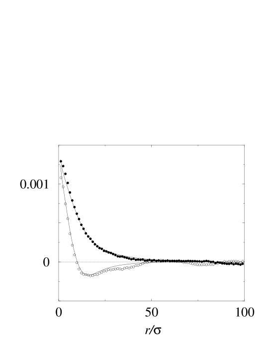
FIG. 8.:

                                                                     

FIG. 9.:

FIG. 10.:

                                                                     

FIG. 11.:

REFERENCES

- [1] T.P.C. van Noije, M.H. Ernst, R. Brito and J.A.G. Orza, Phys. Rev. Lett. 79, 411 (1997).
- [2] T.P.C. van Noije, R. Brito and M.H. Ernst, Phys. Rev. E 57, R4891 (1998).
- [3] T.P.C. van Noije, Ph.D. thesis, Universiteit Utrecht, 1999 (in partial fulfillment of the requirements for a Ph.D. degree at Universiteit Utrecht).
- [4] J.A.G. Orza, R. Brito and M.H. Ernst, unpublished; J.A.G. Orza, Ph.D. thesis (in partial fulfillment of the requirements for a Ph.D. degree at Universidad Complutense, Madrid).
- [5] J.S. Langer, in Solids Far from Equilibrium, Ed. C. Godrèche (Cambridge University Press, 1992).
- [6] Holmes’ Principles of Physical Geology, Ed. D. Duff (Chapman and Hall, Boca Raton, U.S.A., 1994), p. 368.
- [7] I. Goldhirsch and G. Zanetti, Phys. Rev. Lett. 70 1619 (1993).
- [8] I. Goldhirsch, M-L. Tan and G. Zanetti, J. Scient. Comp. 8, 1 (1993).
- [9] S. McNamara, Phys. Fluids A 5, 3056 (1993).
- [10] S. McNamara and W.R. Young, Phys. Rev. E 53, 5089 (1996).
- [11] J.J. Brey, F. Moreno and J.W. Dufty, Phys. Rev. E 54, 445 (1996).
- [12] P. Deltour and J.-L. Barrat, J. Phys. I France 7, 137 (1997).
- [13] J.J. Brey, F. Moreno and M.J. Ruiz-Montero, Phys. Fluids 10, 2965 (1998); 2976 (1998).
- [14] R. Brito and M.H. Ernst, Europhys. Lett. 43, 497 (1998); Int. J. Mod. Phys. C 9, 1339 (1998) (see http://seneca.fis.ucm.es/brito/IHS.html for eigenvectors).
- [15] S. Luding and H.J. Herrmann, Chaos 9 (1999).
- [16] P.K. Haff, J. Fluid Mech. 134, 401 (1983).
- [17] T.P.C. van Noije, M.H. Ernst, E. Trizac and I. Pagonabarraga, Phys. Rev. E 59, 4326 (1999).
- [18] L. Landau and E.M. Lifshitz, Fluid Mechanics (Pergamon Press, 1959).
- [19] U. Frisch, Turbulence: the legacy of A.N. Kolmogorov (Cambridge University Press, 1996).
- [20] D. Rothman, J. Stat. Phys. 56, 517 (1989).
- [21] J.J. Brey, M.J. Ruiz-Montero and D. Cubero, unpublished.
- [22] C.K.K. Lun, S.B. Savage, D.J. Jeffrey and N. Chepurniy, J. Fluid Mech. 140, 223 (1984).
- [23] J.T. Jenkins and M.W. Richman, Arch. Rat. Mech. Anal. 87, 355 (1985).
- [24] S. Chapman and T.G. Cowling, The Mathematical Theory of Non-uniform Gases (Cambridge University Press, 1970).
- [25] A. Goldshtein and M. Shapiro, J. Fluid Mech. 282, 75 (1995).
- [26] N. Sela and I. Goldhirsch, J. Fluid. Mech. 361, 41 (1998).
- [27] J.J. Brey, J.W. Dufty, C.S. Kim and A. Santos, Phys. Rev. E 58, 4638 (1998).
- [28] T.P.C. van Noije and M.H. Ernst, Granular Matter 1, 57 (1998), cond-mat/9803042.
- [29] I. Goldhirsch and T.P.C. van Noije, preprint 1999.
- [30] N.V. Brilliantov and T. Pöschel, cond-mat/9906404.
- [31] J.A.G. Orza, R. Brito, T.P.C. van Noije and M.H. Ernst, Int. J. Mod. Phys. C 8, 953 (1997).
- [32] G.K. Batchelor, The Theory of Homogeneous Turbulence (Cambridge University Press, 1970), Chap. 3.
- [33] G. Grinstein, D.-H. Lee and S. Sachdev, Phys. Rev. Lett. 64, 1927 (1990); G. Grinstein, J. Appl. Phys. 69, 5441 (1991).
- [34] B. Schmittmann and R.K.P. Zia, Statistical mechanics of driven diffusive systems (Academic Press, 1995).
- [35] N.F. Carnahan and K.E. Starling, J. Chem. Phys. 51, 635 (1969).
- [36] L. Verlet and D. Levesque, Mol. Phys. 46, 969 (1982).
- [37] I.S. Gradshteyn and I.M. Ryzhik, Table of Integrals, Series, and Products (Academic Press, New York, 1965).