From Car Parking to Protein Adsorption: An Overview of Sequential Adsorption Processes
Abstract
The adsorption or adhesion of large particles (proteins, colloids, cells, …) at the liquid-solid interface plays an important role in many diverse applications. Despite the apparent complexity of the process, two features are particularly important: 1) the adsorption is often irreversible on experimental time scales and 2) the adsorption rate is limited by geometric blockage from previously adsorbed particles. A coarse-grained description that encompasses these two properties is provided by sequential adsorption models whose simplest example is the random sequential adsorption (RSA) process. In this article, we review the theoretical formalism and tools that allow the systematic study of kinetic and structural aspects of these sequential adsorption models. We also show how the reference RSA model may be generalized to account for a variety of experimental features including particle anisotropy, polydispersity, bulk diffusive transport, gravitational effects, surface-induced conformational and orientational change, desorption, and multilayer formation. In all cases, the significant theoretical results are presented and their accuracy (compared to computer simulation) and applicability (compared to experiment) are discussed.
I Introduction
The adsorption of large particles (proteins, viruses, bacteria, colloids, macromolecules) at the liquid-solid interface has received considerable theoretical and experimental attention in recent years. Among the many issues pertaining to this problem, we address in this review the consequences on the adsorption kinetics and the adsorbed layer structure of two key features: i) the absence of reversibility and ii) the deceleration of adsorption due to surface exclusion from previously adsorbed particles[1, 2, 3, 4, 5, 6]. We choose as a starting point a mesoscopic approach, where atomic-level detail is coarse-grained and incorporated as a set of effective parameters such as rate constants, particle shapes and sizes, effective interparticle interaction parameters, etc…The two essential features listed above are well accounted for in sequential adsorption models[7, 8]; these will be the central topic of this review.
The outline of our review is as follows. In section II, we introduce the simplest of sequential adsorption processes, the random sequential adsorption model (RSA), and its one-dimensional version, the car parking problem. Since these processes result in structures that are generally far from equilibrium, the well-developed methods of liquid-state statistical mechanics are not directly applicable. We present, in section III, the formalism and principal theoretical tools that we have developed for describing the kinetics of the adsorption processes and the structure of the adsorbed layers. The next sections are devoted to extensions of these methods to processes involving additional physical features. In section IV, we consider the adsorption of nonspherical particles and of mixtures and in section V, we address bulk transport issues such as particle diffusion and the influence of the gravitational field. In section VI, we treat surface-induced events, like conformational and orientational changes of the particles and in section VII, we introduce partial reversibility produced by desorption. Finally, we discuss multilayer formation in section VIII.
II RSA: a reference model
The random sequential adsorption model, the prototype for sequential addition processes, is a stochastic process in which “hard” particles are added sequentially to a -dimensional volume at random positions with the condition that no trial particle can overlap previously inserted ones.
A The car parking problem
The one-dimensional version of the model, known as the car parking problem, was first introduced by A. Rényi[9], a Hungarian mathematician. Consider an infinite line, assumed empty at . Hard rods of length are dropped randomly and sequentially at rate onto the line, and are adsorbed only if they do not overlap previously adsorbed rods. Otherwise, they are rejected. If denotes the number density of particles on the line at time , the kinetics of this process is governed by the equation
| (1) |
where , the insertion probability at time , is the fraction of the substrate that is available for the insertion of a new particle. To calculate this quantity, it is convenient to introduce the gap distribution function , which is defined so that represents the density of voids of length between and at time . For a given void of length , the available length for inserting a new particle is , and therefore the available line function is merely the sum over the number density of available intervals, i.e. :
| (2) |
Since each interval corresponds to one particle, the number density of particles can be expressed as
| (3) |
whereas the uncovered line is related to by
| (4) |
These two equations, Eqs. (3- 4), represents two sum rules for the gap distribution function. During the process, the gap distribution function evolves as
| (5) |
where is the unit step function. The first term of the right-hand side of Eq. (5) (destruction term) corresponds to the insertion of a particle within the gap of length (for ), whereas the second term (creation term) corresponds to the insertion of particle in a gap of length . The factor is due to the two possibilities of creating a length from a larger interval . It is worth noting that the time evolution of is entirely determined by intervals larger than . We now have a closed set of equations, which results from the fact that the adsorption of a particle in one gap has no effect on other gaps. The above equations can be solved by introducing the ansatz[10]
| (6) |
which leads to
| (7) |
Inserting Eqs. (6) and (7) , one obtains for and integrating Eq. (5) with the solution of for finally gives for ,
| (8) |
The three equations, (1), (3) or (4), all lead to the same result for the number density ,
| (9) |
which was first derived by Rényi[9].
A first nontrivial property of the model is that the process reaches a “jamming limit” (when ) at which the density saturates at a value ; this value is significantly lower than the closed-packed density () that is expected when the surface is allowed to restructure between adsorption steps. Moreover, it is easy to show that the jamming limit depends upon the initial configuration, here an empty line. In contrast, the final state of an equilibrium system is determined solely by the chemical potential and has no memory of the initial state. The long-time kinetics, during which a small number of adsorption events occurs, can be obtained from Eq. (9) and are seen to display a power-law behavior.
| (10) |
where is the Euler constant.
The structure of configurations generated by this irreversible process has several noticeable properties. At saturation, the gap distribution function shows a logarithmic divergence at contact, ,
| (11) |
The correlations between pairs of particles are extremely weak at long distances. The pair correlation function behaves at long distances as
| (12) |
where is the Gamma function, i.e., it decays super-exponentially in contrast with the characteristic exponential decay of equilibrium systems[11].
B Two-dimensional sequential adsorption
The RSA model can be studied in two dimensions, which represents the physical dimension for adsorption problems. Since the RSA process generates random disordered configurations of “hard particles”, a statistical geometric approach is useful for describing the system. For a given time , or equivalently a given density , it is convenient to introduce the set of particle density functions , where denote the positions of the particles, that characterize completely the configuration of particles.
The time evolution of the density is still given by Eq. (1), where denotes the available fraction of the surface for the insertion of a new particle. When the particles are hard disks, has a simple geometrical interpretation: It represents the probability of finding a circular cavity of diameter equal to twice the particle diameter, that is centered at , and is free of particle centers[12, 13, 14]
| (13) |
where denotes a cavity (as defined above) and is the Mayer function for non overlapping hard particles:
| (14) | |||||
| (15) |
where is the diameter of the hard spherical particles. (Note that because of the macroscopic uniformity of the system, is independent of the position , i.e., .) The terms of the sum in the right-hand side of Eq. (13) can be interpreted geometrically : the first term, which is equal to one, corresponds to the certain acceptance of particles added to an empty surface. The second (negative) term subtracts the fraction of the surface occupied by exclusion disks in which no new particle center can be placed. The third (positive) term corrects for the fact that two exclusion disks may overlap, etc… For hard-core interactions, the sum is always finite since the number of non-overlapping particles located at a distance less than the particle diameter from a given point is finite. For instance, for hard disks in two dimensions, only six first terms have a nonzero contribution to Eq. (13).
Higher order density functions can be systematically defined. For instance, represents the density of finding one (unspecified) particle at the point and a cavity of diameter free of particle centers at the point . More generally, one can introduce as the probability density of finding (unspecified) particles at the points and a cavity of diameter free of particle centers at the point ,
| (17) | |||||
For a RSA process, the insertion of a new particle amounts to finding a cavity of diameter for a given set of previously adsorbed particles. The kinetic equation for the density, Eq. (1), can be generalized to higher order density functions,
| (18) |
or, by using Eq. (1),
| (19) |
The exact and infinite hierarchy of equations cannot be solved (nor is it possible in the equilibrium case), but approximate solutions and computer simulations (both to be detailed below) provide a good description of the process.
The main features observed in the one-dimensional car parking problem persist in higher dimensions: existence of a jamming limit at which the density of adsorbed particles saturates (in , [15, 16]), slow kinetics when approaching jamming (in , [15]), logarithmic divergence at contact of the pair correlations at saturation, configurations of adsorbed particles that differ from those characteristic of an equilibrated system. The qualitative and quantitative relevance of two-dimensional RSA for describing the adsorption of macromolecules at liquid-solid interfaces has been demonstrated in several experiments on proteins[1, 17] and colloidal particles[2, 6, 18, 19, 20].
III Theoretical formalism and tools
A Statistical mechanics of sequential adsorption systems
Consider a system of particles in a -dimensional volume (in practice, adsorption involves ). For simplicity, we assume that the particles are identical and interact through a pairwise-additive spherically-symmetric potential. Generalization to mixtures, nonspherical particles and non pairwise-additive potentials is, conceptually at least, straightforward (see below). If the system of particles is at equilibrium at a given temperature , the probability density, associated with finding the particles in a configuration with one (unspecified) particle whose center is an infinitesimal volume element around position ,…,one (unspecified) particle whose center is an infinitesimal volume element around position is given by the Gibbs distribution for the canonical ensemble,
| (20) |
where , is the Boltzmann constant, is the pair potential, and is the configurational integral defined by
| (21) |
All the powerful tools of equilibrium statistical mechanics and the connection to thermodynamics derive from the Gibbs distribution. Consider now a situation in which the configuration of particles does not correspond to thermal equilibrium, but is generated by a sequential adsorption process. More specifically, we consider a “cooperative sequential adsorption” (CSA) that is a simple generalization of the random sequential adsorption process introduced above. In this process, the rate of adsorption of a new particle in a given configuration of pre-adsorbed particles is proportional to a Boltzmann factor involving the interaction energy between the new particle at the chosen position and all preadsorbed particles. If denotes the position of the preadsorbed particles, adsorption of a particle at position is given by
| (22) |
where is the rate of adsorption of a particle in an empty -dimensional volume. What is the probability of finding a given configuration with a total number of particles at which is generated by this cooperative sequential adsorption, irrespective of the time required? It is clear that the intrinsic irreversibility, resulting from the fact that once a particle is adsorbed it can no longer move or desorb, creates a strong memory effect. As a result, one must take into account the order in which the positions have been filled by particle centers and consider the sequences of insertion that lead to a given configuration of particles at . With the rate given by Eq. (22) and the definition , one obtains the following probability density
| (23) |
where the sum is over all permutations of and where we have used that . (One easily checks that the normalization condition is satisfied). Eq. (23) is the CSA counterpart of the Gibbs distribution for equilibrium systems, Eq. (20). In a thermally equilibrated system, Eq. (20) implies that all configurations having the same energy are equiprobable. On the other hand, in a sequential adsorption process there is a bias that favors some configurations over others among all those that have the same energy: this results from the fact that in Eq. (23), the factor depends on the positions (for ). This feature has been already noted by Widom[21] in the example of three hard spheres added to a large volume. The seemingly formal difference between the equilibrium Gibbs distribution, Eq. (20), and the CSA distribution, Eq. (23), has important consequences. Some of the dramatic ones are that the CSA systems are characterized by the existence of a jamming limit where the density of adsorbed particles (for particles possessing a hard core) reaches a saturation value that is significantly less than the optimum filling (as in RSA, cf section II) and the absence of thermodynamic phase transitions***Geometric phase transitions such a percolation phenomena are still possible, see section V B.. This latter feature results from the infinite memory of the adsorption process and is illustrated in Fig 1. In the figure, we compare two typical configurations of hard nonspherical two dimensional particles (disco-rectangles , i.e. a planar spherocylinder, with an aspect ratio of ) on a plane at the same surface density (or coverage), one being an equilibrium configuration, the other being generated by RSA. At the chosen coverage of , the equilibrium configuration is in a nematic phase with long range orientational order (the transition from the disordered to nematic occurs for ), whereas the RSA configuration is at saturation in a disordered state.
The existence of a well-defined probability density for configurations of particles produced by sequential adsorption in a -dimensional volume at a given temperature , as in Eq. (23), makes a “statistical mechanical” approach possible, but the complicated form of the probability density imposes a nontrivial generalization of the equilibrium formalism.
The kinetics of a sequential adsorption process, as well as the characteristics of the configurations of adsorbed particles, can be obtained from a knowledge of the grand ensemble analog of the “canonical” probability density introduced above, , which is associated with finding a configuration of adsorbed particles positioned at at time . However, the expression of this quantity is quite intricate, and it is convenient to derive directly kinetic equations describing the time evolution of the infinite set of -particle densities, . ( is associated with the probability of simultaneously finding an (unspecified) particle at , another at ,…, and one at , irrespective of the remaining particles and is thus obtained from the ’s for by integrating over the positions of remaining particles. This derivation has been done in section II B for the RSA of hard particles by means of statistical geometric arguments. The result can be generalized for all sorts of cooperative sequential adsorption processes (as well as processes involving desorption and other mechanisms, see the next section). Consider a cooperative sequential adsorption similar to that described above with an adsorption rate that generalizes Eq. (22), namely
| (24) | |||||
| (25) |
where is a short-hand notation for center-of-mass position and orientation j and is the interaction energy between an incoming particle at position with orientation n+1 and preadsorbed particles characterized by . There is no need here to assume pairwise additivity or spherical symmetry for the interaction potential.
The time evolution of the particle density, which, for macroscopically homogeneous (i.e. both uniform and isotropic) systems considered here, is equal to the average density of adsorbed particles , is governed by the following kinetic equation:
| (26) |
where is the probability of inserting a new particle at the position with an orientation 1. (Note that because of the homogeneity of the system, one can average as well over and 1). Introducing the Ursell (or “cluster”) functions associated with the ’s,
| (27) |
where the second sum in the right-hand side of the above equation is over all distinct -tuplets chosen from , and recalling that for sequential adsorption processes there is a one-to-one mapping between reduced time, , and density, , one generalizes Eq. (13) as follows:
| (28) |
where the integral involves integration over both center-of-mass positions and orientations. For a pairwise additive potential, it is easy to show that the Ursell function is just a product of conventional Mayer functions , , and that Eq. (28) reduces to Eq. (13) for simple RSA. For higher-order particle densities, generalizing Eq. (19) leads in a similar way to
| (29) |
with
| (30) |
where the ’s are generalized Ursell functions defined by
| (31) |
Again, for pairwise additive potentials, the generalized Ursell functions reduce to products of Mayer functions. (In section V B, we shall consider a process with non-pairwise additive potentials.)
The above hierarchy of equations for the -particle densities is the counterpart for cooperative sequential adsorption processes of the Kirkwood-Salsburg hierarchy for equilibrium systems. The latter reads
| (32) | |||||
| (33) |
where the ’s are given by the same expression as in Eqs. (28) and (30). The comparison of Eqs. (29) and (32) illustrates again the difference between CSA and equilibrium systems.
The Kirkwood-Salsburg hierarchy for CSA processes, Eqs. (26)- (30), is a good starting point for generating diagrammatic expansions[14]. These can be used to formulate various approximate descriptions, such as low-density expansions for the adsorption probabilities and integral equations for the pair correlations, that parallel those used in equilibrium statistical mechanics of fluids. In the case of pairwise additive potentials, diagrammatic expansions are also conveniently derived by using the “replica trick” developed for spin glass models[22]. The trick relates the probability distribution for CSA and RSA configurations of particles to the Gibbs distribution of a fictitious equilibrium system with replicas of particle , replicas of particle ,…, replicas of particle , in the limit ,,.[23]
B Approximation scheme
There is, unfortunately, no exact solution to the sequential adsorption problem when the dimensionality of the substrate is two or more, (the one-dimensional case will be discussed below). To describe the kinetics of the adsorption process and of the structure of the adsorbed configuration, one can use computer simulation (see below). In addition, it is also fruitful to develop approximate treatments that allow one to study a wide range of control parameters and a variety of interactions, external fields, and mechanisms. To do so, it is instructive to consider configurations of hard disks generated by RSA at different stages of the process. This is illustrated in Fig. 2a-c. Also shown in white on the figures is the region that is available for the insertion of a new disk center and whose area gives the adsorption probability (correspondingly, the region in gray is that part of the surface which is excluded to the center of a new disk, over and above the region covered by the adsorbed disks themselves that is shown in black, cf section II B). At low surface coverage, corresponding to short times, the available surface percolates through the whole space and adsorption is locally prohibited by groups involving only a small number of preadsorbed disks. When the coverage increases, the available surface diminishes and no longer percolates. Finally, close to the jamming limit (the saturation coverage is ), the available surface reduces to small, isolated regions that can accommodate only one additional disk. This suggests that different approximations must be used for describing the different stages of the process.
Consider first the last-stage, long-time, regime that corresponds to the asymptotic approach to the jamming limit. Note that the existence of such a jamming limit is a feature of all sequential adsorption processes, be they random or cooperative, provided the adsorbing particles possess a “hard core” that results in an exclusion or blocking effect. When the surface coverage is sufficiently high, this hard-core interaction dominates all additional “soft” potentials describing for instance dispersion and electrostatic interactions. (The case of “singular” additional potentials such as those encountered for systems of sticky disks and in the description of generalized ballistic deposition (see section V B) is different). In the asymptotic regime near the jamming limit, the surface available for adding new particles is composed, as shown above, of small isolated “targets”, whose number exactly provides the number of particles that will still be adsorbed before reaching saturation. Due to the irreversibility and the infinite memory of the process, the asymptotic kinetics is simply related to the rate of disappearance and the statistics of the targets. The standard arguments for the RSA of spherical particles have been put forward by Pomeau[24] and Swendsen[25]. Consider a typical target at time that is characterized by a small linear scale so that the area available for the center of a new disk goes as in dimensions (and for general dimension ) (see Fig. 3). The rate of disappearance of such a target is proportional to its surface area, hence to ; as a consequence, the number density of targets characterized by a linear size , decays exponentially in time according to
| (34) |
where is a crossover time that marks the beginning of the asymptotic regime and is a mean shape factor (besides , the geometric characteristics of the targets are irrelevant). Making the reasonable assumption that goes to a nonzero value when , one then obtains that the difference in density of adsorbed particles between time and saturation () is given by
| (35) | |||||
| (36) |
where is an (unimportant) upper cutoff. The approach to saturation is thus very slow in RSA processes and is described by a power law in time (when , one recovers the exact result, cf section II A). The same line of reasoning permits one to show that the pair correlation function at saturation has a logarithmic divergence when two disks (or, more generally, two dimensional spherical particles) approach contact, a result that is also obtained exactly in one dimension (cf section II A). The arguments in terms of small, isolated targets can be generalized to all CSA and RSA processes involving particles with a hard core. The key property is the rate of disappearance of targets when their linear size goes to zero. If this rate goes to a nonzero limit, as in the case of generalized ballistic deposition (which corresponds to singular sticky potentials, cf section V B) and of a mixture involving point-like particles[26], the approach to saturation is fast and is essentially exponential. If the rate goes to zero, generally as where is the number of degrees of freedom for the adsorbing species, the approach is again a power-law, : for instance, in two dimensions, for non spherical (unoriented) particles[27, 28] as well as for a continuously polydisperse mixture of disks[29], whereas for a monodisperse system of disks. Note that the above results are valid for irreversible adsorption in which once adsorbed, the particles stay fixed. A quite different behavior is observed when particles are allowed to desorb from the surface (see section VII B).
In the low and intermediate density regime (Figs. 2a and 2b), one expects that the approximation employed in the statistical mechanical theory of equilibrium fluids can, mutatis mutandis, be useful as well for describing systems of particles produced by sequential adsorption. In particular, this is the case for low-density expansions, somewhat analogous to the standard virial expansion for the imperfect gas[30]. As mentioned above, such expansions can be generated either order by order from the Kirkwood-Salsburg-like hierarchy or directly from the diagrammatic series when they are available (e.g., for pairwise additive potentials). For instance, the adsorption probability for the RSA of hard disks onto a plane is given by
| (37) |
where is the hard-disk diameter and is the surface coverage. As noted before (section III A), this expansion coincides with its equilibrium counterpart at order , but departs from it at the next order (in general, ). Similar formulas have been derived for the adsorption of hard convex objects of various shapes, for mixtures, and for sequential processes involving cooperative effects and competing mechanisms (see below). For cases involving “soft” (i.e continuous in the configurational variables) interaction potentials in addition to hard cores, the computation of the coefficients is always numerical since it requires more than geometric considerations. However, one can again fruitfully borrow ideas that have proven efficient in equilibrium statistical mechanics[30]: weak attractive potentials can be treated as perturbations and spherically-symmetric soft repulsive potentials can be approximately replaced by a hard-core potential with a suitably chosen effective diameter that depends on both density and temperature[6, 31].
Even for hard-core exclusion interactions, calculating the coefficients rapidly becomes intractable as the order in density increases. For hard disks, the fourth-order term has been obtained and for parallel hard squares, the sixth-order term, but these are exceptions, and in practice only coefficients up to (or ) have been calculated analytically. This unfortunately restricts the range of density over which the truncated expansion is accurate. It is possible, however, to enhance the convergence of the low-density expansion by building interpolation formulas that incorporate the known asymptotic behavior. For instance, in the case of the RSA of hard disks, the result converts, through the use of the kinetic equation , to when . By employing standard techniques such as Padé approximants[32, 33, 34], e.g.,
| (38) |
where the coefficients are determined by expanding in coverage (or density) and matching term by term to the exact expansion, Eq. (37), one obtains an improved description of the kinetics over the whole process. In particular, expressions such as Eq. (38) provide estimates of the saturation coverage . The procedure works very well for the RSA of hard dimensional spheres and dimensional parallel hard cubes: cf Table I. For more complicated shapes and more complicated cooperative processes (see below), the results are fair, but not as good. This trend can usually be rationalized by invoking the appearance of an additional regime in the process (see, for instance, the case of elongated nonspherical particles with random orientations discussed in section IV A).
The approximation scheme just described focuses on the kinetics of the process at the level of the density of adsorbed particles (or surface coverage). However, valuable insight on the adsorption process is gained by a proper description of the spatial correlations among adsorbed particles. Actually, studying the structure of the adsorbed layer can facilitate the discrimination between different hypothesized model descriptions of real adsorption situations[1, 6, 20]. In this regard, it is interesting to develop approximate treatments for obtaining the pair correlation function in configurations of particles generated by sequential adsorption. As in equilibrium statistical mechanics, the most obvious route is to derive integral equations for the pair correlations, and this can be done by making approximations in the diagrammatic expansions, as obtained for instance from the Kirkwood-Salsburg-like hierarchy presented above. As an example, the analog of the celebrated Percus-Yevick integral equation for dimensional equilibrium hard-sphere fluids[30] has been studied for the RSA case[35]. The result for the pair correlation function for an adsorbed layer of hard disks is illustrated in Fig 4. The description is good at intermediate surface coverage, but, as expected, it deteriorates in the asymptotic regime near saturation; the approximation fails to reproduce the logarithmic divergence at contact (see section II B), but it captures the rapid, super-exponential decay of the spatial correlations with distance that is typical of sequential adsorption processes[8, 11].
C Usefulness of one-dimensional models
The vast majority of real situations in which large particles (proteins, cells, colloids,…) adsorb at a liquid/solid interface correspond to a two-dimensional substrate (that, for sake of simplicity, we consider flat and uniform in this whole review). Why therefore should one study one-dimensional models? Equilibrium statistical mechanics seems to teach us that one-dimensional systems have very little relevance to physical two- and three-dimensional fluids; indeed, no thermodynamic phase transitions are possible in one dimension whereas they are a key phenomenon of real fluids. The situation is, however, different for sequential adsorption processes. First, as already stressed, there is no thermodynamic phase transition in the adsorbed layer, regardless of its dimensionality. Second, the main features of the phenomenology of sequential adsorption processes, such as the existence of a jamming limit and of a well-characterized asymptotic approach toward saturation, the short (super-exponentially) decay of the spatial correlations among adsorbed particles, and many other properties that may depend upon the specific process under study (see the following sections), are independent of space dimensionality. One-dimensional sequential adsorption models already have the ingredients, partial or total irreversibility with the associated memory effect, exclusion or blocking phenomena, that make their behavior nontrivial and qualitatively similar to that observed in higher dimensions. There are of course quantitative changes. For instance, a sequential adsorption process with hard objects is less and less efficient as the dimension increases. (For the RSA of spherical particles, for , for , for , etc; it is, however, interesting to note that, as a rule of thumb, the saturation coverage in dimensions is rather well approximated by that in one dimension raised to power [36]).
An additional motivation for studying one-dimensional models is that they are often amenable to exact analytical solutions, as illustrated by the case of the car parking problem (see section II A). The underlying reason for solvability is a shielding property[8], that is generally found only in one dimension. The shielding property in one dimension means that an empty interval of a minimum, finite length separates the substrate into two disconnected regions such that adsorption in one region is not affected by the configuration of particles in the other region[8]. As a result, a closed system involving only a finite number of kinetic equations can be written and, often, solved. Further examples will be given in sections V and VI.
D Monte Carlo algorithms
Computer simulation provides additional information on sequential adsorption processes. It was from simulation results, for instance, that Feder first observed the characteristic power-law kinetics at long times[15]. The basic procedure for a Monte Carlo simulation of a sequential adsorption process with hard-core particles is the following: at each step, one attempts to place a particle in the simulation cell with periodic boundary conditions, at positions sampled from a uniform probability distribution. Because of the finite range, hard-core interaction between particles, it is advantageous to employ a grid construction[16]. The computer time then depends on the number of particles instead of the square of the number. Moreover, close to the jamming limit the process is dominated by very few successful events of adsorption and accelerating procedures have been introduced. Indeed, at long times, the available surface for inserting new particles is very small compared to the simulation cell. If the grid cell element is chosen for accommodating only one particle, the algorithm can be improved as follows: first, an unoccupied grid element is chosen at random and a second random number determines the trial position within the vacant grid element; the time is then incremented by an amount where is the total number of grid elements in the simulation cell and is number of vacant grid elements at a given density[37, 38]. (The procedure accelerates significantly the simulation, but it may occur that in the last stage of the process, the surface which is the sum of the grid elements remaining vacant exceeds largely the available surface for inserting new particles and many unsuccessful attempts still slow down the simulation). Event-driven algorithms have been used in various adsorption models (RSA of nonspherical particles[38], polymer adsorption[39]). Moreover, in some cases, e.g., in one dimension, the available surface can be determined exactly, and a trial position can be always chosen within the available surface such that no rejection (or wasted time) occurs along the simulation. The procedure leads to a correct result provided that the time is incremented by the ratio of the system size to the available surface. It can also be used in the simulation of processes involving desorption (see Section VII C).
IV Adsorption of nonspherical particles and mixtures
A RSA of anisotropic particles
Biological molecules have in general a nonspherical shape and they adsorb in an irreversible way when the area of the surface they have in contact with the substrate is maximum. Experimentally, Schaaf et. al[40] found that the maximum coverage of the substrate they were able to obtain in the adsorption of fibrinogen (a nonspherical protein with aspect ratio of approximately ) was around , i.e. less than the saturation coverage predicted by the RSA of hard disks () and observed in experiments involving fairly spherical globular proteins[1, 15, 17]. (A similar effect was observed for adsorption of albumin[41].) A simple way to account for these effects consists in considering the irreversible adsorption of anisotropic particles onto a surface with the RSA rules generalized so that the positions and the orientations of the adsorbing particles are chosen randomly from uniform distributions (for generalizations, see Section VI. We and other authors[27, 28, 42, 43, 44, 45, 46, 47, 48] have performed this study for hard convex bodies of different shapes: ellipses, squares, disco-rectangles (i.e. “ spherocylinders”). The relevant questions include the following:
-
1.
What is the influence of the aspect ratio on the saturation coverage of the substrate?
-
2.
What is the dependence on the particle shape of the kinetics (short and long times)?
-
3.
What are the similarities and differences between the RSA generated configurations and equilibrium configurations at the same surface coverage?
The hard convex bodies mentioned above are characterized by one parameter which is the aspect ratio, : for ellipses and disco-rectangles, is the ratio of the long axis to the short axis and for rectangles is the ratio of the length to the width. Both disco-rectangles and ellipses reduce to a disk when , while rectangles tend to a square (i.e. an anisotropic object) in the same limit. Fig. 5 displays the saturation coverage obtained by computer simulation of two-dimensional RSA as a function of the inverse aspect ratio, , for various shapes. Three main conclusions can be drawn from the results: (i) for the three different shapes, the maximum coverage is obtained for a value of close to 2; (ii) the maximum coverage for ellipses and disco-rectangles (for ) is larger than that for disks; and (iii), for all objects considered here, the saturation coverage goes to zero when the aspect ratio goes to infinity, seemingly with a power law dependence. It is also interesting to note that for - (typical of fibrinogen, see above), the saturation coverage falls below the hard-disk value and is close to .
As far as the kinetics are concerned, computer simulation also showed that the approach toward saturation is slower for anisotropic objects than it is for disks[27]. From a geometric analysis of the available surface, Talbot et al.[27] showed that the long-time kinetics results from adsorption of particles in two types of targets, the larger ones being independent of the orientation of the trial particle (nonselective targets) and the smaller ones corresponding to the insertion of a particle with a small range of possible orientations (selective targets). To minimize size effects while still retaining the effect of anisotropy, Viot and Tarjus [28] performed extensive simulations of the RSA of unoriented squares, and the results clearly showed that the asymptotic approach follows a power law with an exponent equal to . For ellipses and disco-rectangles with moderate and large aspect ratios, the long-time kinetics are described by the same power law, but the crossover time beyond which the asymptotic kinetics sets in increases with . For weakly elongated objects, by introducing a small anisotropy parameter, , it can be shown that the long-time kinetics follows the equation[47]
| (39) |
where and is a positive constant. Eq. (39) can be simplified in the two limits and . The long-time kinetics thus consists of two consecutive asymptotic regimes. First, for , one has a behavior and for this regime vanishes and a behavior emerges. This last regime disappears and the contribution to the coverage goes to zero when the aspect ratio goes to one. Simulations have been performed for weakly elongated objects and only an effective exponent between and has been measured[47]. (To observe numerically a clear separation of these two critical regimes, simulations of very slightly elongated particles should be performed.)
The low-coverage expansion of the available surface function permits, as shown in section III A, a systematic description for low and, somewhat intermediate coverages. To third order, one has
| (40) |
where denotes the th equilibrium virial coefficient[30] and is the specific RSA coefficient which can be expressed in terms of Mayer diagrams[46]. All coefficients must be calculated numerically in general[44], except the second virial coefficient for which an analytical formula is known[49]. The comparison with simulation results shows that the third-order expansion provides a good description as long as is not too small. It is worth noting that the range of usefulness of the density expansion diminishes when the aspect ratio increases. Even at low coverage, decreases markedly when increases, which means that adsorption of very elongated particles rapidly becomes difficult. An intermediate regime appears before the asymptotic regime, in which the longest linear size of the particles is responsible for many rejections of trial particles in the process. As displayed in Fig. 1, this regime leads to the formation of a local order whose (linear) domain size is given by the length of the particle long axis. The feature becomes more pronounced when the aspect ratio becomes larger. This regime cannot be described by a low-density expansion whose validity (or quality) range is of order . (Notice that for equilibrium systems, a virial expansion is also unable to describe the isotropic-nematic transition.) To understand the emergence of this third regime, it is useful to consider the adsorption of infinitely thin needles whose length corresponds to that of the long axis of elongated particles. For needles, which do not have a proper area, no saturation is reached and the number density of needles increases algebraically with time[45]. By studying the one-dimensional problem, two of us[45] showed that the RSA of needles can be mapped at long times onto a solvable two variable fragmentation model[45, 50] and that the density of needles increases asymptotically as
| (41) |
The same algebraic law is expected to hold in two dimension, as is confirmed by computer simulations[51, 52].
Following the procedure described in section III B, approximation schemes can be constructed by combining low-density expansions and asymptotic regimes. For weakly and moderately elongated particles ( ), a fit of the form of Eq. (38) gives results which are indistinguishable from the simulation data during most of the process. However, the predicted saturation coverage is overestimated by the fitting formula[46].
For very elongated particles, a more efficient approximation scheme can be built. From the discussion above, it can be assumed that the filling process is mainly composed of two critical regimes: a needle-like regime followed by the true asymptotic regime. Matching the two behaviors leads to the following result,
| (42) |
and the crossover time between the two regimes is
| (43) |
when . These two results are well supported by simulations: for elongated rectangles, Vigil and Ziff[42, 52] obtained an algebraic law , whereas the value of the exact exponent of Eq. (42) is . The increase in crossover time has also been reported but not quantitatively estimated[43].
A structural analysis of the configurations of anisotropic particles generated by RSA has been performed by considering the pair correlation function[48]. For anisotropic hard-core particles in two dimensions, the pair correlation depends on three variables: the distance between the two particles and the orientation of each particle with respect the interparticle vector. The center-to-center pair correlation function , which is the average over the orientations of two particles, i.e. has no orientational dependence, already provides useful information on the structure. In particular, the highest peak in is for a distance close to when , whereas the peak shifts towards with a secondary weak peak emerging for distances close to when (all distances are measured in units of the short axis). These results show that the most probable relative orientation of two particles evolves from perpendicular to parallel when the anisotropy parameter becomes larger. Although the center-to-center pair correlation function is always finite at contact, one observes a logarithmic divergence of the surface-to-surface pair correlation function at saturation[48]. This is reminiscent of the behavior observed in the RSA of spherical particles. As already stressed, nematic order is never observed, regardless of the aspect ratio.
B RSA of mixtures
For a general mixture of components of arbitrarily hard particles adsorbing irreversibly on a planar surface, one would like to be able to predict the time dependent and saturation coverages. Even in one-dimension, this is a challenging problem. However, one can deduce the behavior in some limiting cases.
The RSA of a binary mixture of hard disks is characterized by two parameters: , where and are the adsorption rates of the components on an empty surface, and the diameter ratio . Talbot and Schaaf [53] analyzed the case of a binary mixture of hard disks of greatly differing diameters, . The time-dependent coverages can be obtained from the numerical solution of two coupled first-order differential equations,
| (44) |
| (45) |
where and is the effective coverage of the smaller disks. As long as is sufficiently small, depends only on and the large disks approach their saturation coverage exponentially. The small disks then behave essentially as a one-component system in a reduced area, approaching their jamming limit coverage according to the usual algebraic power law, [53]. The final combined saturation coverage is accurately given by
| (46) |
where .
Tarjus and Talbot examined the asymptotic approach to the jamming limit of a continuous polydisperse mixture [29]. The adsorption rate of a particle of radius on an empty surface, , is assumed to be continuous for and zero otherwise. As in the monocomponent system (section III B), the asymptotic kinetics are determined by the filling of isolated target areas. If is different from zero then it follows that the jamming limit is approached as
| (47) |
This is consistent with the idea that the exponent is the inverse of the number of degrees of freedom of the adsorbing species: two translational, plus one corresponding to the continuous distribution of particle diameters (see also section IV A for anisotropic particles). Note that if then the exponent is determined by the order of the first non-vanishing derivative of at [29].
V Bulk transport issues
In the simple RSA model the position of the trial particle is selected from a uniform, random distribution. While this simple choice facilitates both simulation and analytic solutions in come cases, it is not clear that it is always consistent with the transport mechanism of the particle from the bulk to the vicinity of the adsorption surface.
An adsorbing particle is in general subject to Brownian, gravitational and hydrodynamic forces, as well as specific interactions with the adsorbing surface and the pre-adsorbed particles. Examples of the latter include van der Waals, electrostatic and short range repulsions.
A substantial body of work has addressed the issue of the effect of the transport mechanism of the adsorbing particles on the adsorption kinetics and the resulting structure of the deposited particle configurations. In particular, two limiting cases of interest are Diffusion Random Sequential Adsorption (DRSA) and the Ballistic Deposition (BD). In the former the transport mechanism is pure diffusion, while in the latter gravitational forces are dominant. For spherical particles, one can define a dimensionless gravity number (proportional to the Péclet number)
| (48) |
where is the difference between the particle and solution mass density, the acceleration due to the gravity, is the particle diameter, is the Boltzmann constant, and T is the temperature. The limits and correspond to the BD and DRSA models, respectively.
A Bulk diffusion
Schaaf et al. analyzed the effect of diffusion on the asymptotic kinetics [56]. They found that the presence of bulk diffusion modifies the asymptotic kinetics,
| (49) |
The saturation coverage is approached more rapidly than in simple RSA due to a funneling effect of the pre-adsorbed particles forming the target. Yet, this power law has never been observed experimentally. This may result from the presence of hydrodynamic interactions between the diffusing particles and the particles on the surface, interactions that are neglected in the diffusion RSA model and that may modify the kinetics and the structure of the adsorbed layer[57, 58, 59].
Senger et al [60, 61] examined the kinetics and saturation coverage of the DRSA process by simulating the random walk of a spherical particle of radius on a cubic lattice with a lattice parameter . Each trajectory starts from a randomly selected lattice site in a plane at height . A particle is adsorbed, and remains permanently fixed, once its center reaches the plane . If the particle reaches the plane it is considered lost to the bulk and a new trajectory is initiated. At each Brownian step, the particle moves to one of six neighboring sites with equal probability. If the selected displacement results in an overlap with a preadsorbed particle, the particle is returned to its initial position and a new direction is chosen.
The principal result of the simulations was that to within the statistical error, the coverage and structure of the adsorbed particle configurations generated by a DRSA process are identical to those of the simple RSA model. In order to gain insight into this unexpected result, various one-dimensional models were studied. In particular, the generalized parking process proposed by two of us[62] proved useful in understanding the effect of the transport mechanism.
In dimensions, the kinetic equation describing the generalized parking process is
| (50) |
Where the rate of adsorption per unit length in a gap of size is denoted by . In simple RSA, where is the Heaviside unit step function.
In the generalized parking process, the rate of deposition of a particle in a gap depends on the width of the gap, but is uniform within the gap. It has been shown that all generalized parking processes have the same jamming limit coverage. Here we reproduce the argument given by Bafaluy et al. [63]. The problem is to determine the number, of particles adsorbed on a line segment of length after an infinite time. Insertion of one particle into this gap leads to two new gaps of length and so one has the following recursion formula:
| (51) |
where is the probability that insertion of a disk into the gap of length produces gaps of length and . In all generalized parking processes, including simple RSA,
| (52) |
since, by definition, the trial particle arrives randomly and uniformly in the gap. Thus, the final state of the system does not depend on and we conclude that all generalized parking processes have the same jamming limit. The kinetics, of course, can vary greatly depending on the form of .
The story is not yet complete, however, since a careful simulation study revealed that the saturation coverage of 1D DRSA [64] at is slightly larger than that of 1D RSA (). This difference is a result of the non-uniform flux of particles at the surface. Eq. (50) can be modified to allow for a non-uniform distribution of incoming particles:
| (53) |
where is the total rate that gaps of length are destroyed by addition of a new particle and is the probability per unit length per unit time that deposition of a disk in a gap of length produces gaps of length and . One can also obtain information about the jammed state without solving Eq. (53) directly with an approach similar to that described earlier for the generalized (uniform) parking process. It is possible to obtain an analytic expression for the flux of particles on a line segment bounded by two preadsorbed disks [63] and the result obtained for the jamming coverage is equal to the simulated value within the confidence interval. More recent work has examined situations where both gravity and and diffusion play a role[65].
B Ballistic transport and generalizations
The ballistic deposition model describes situations in which the transport is dominated by gravitational effects, corresponding to large values of (Eq. (48)). Adsorbing particles follow linear trajectories from the bulk to the adsorption surface. If the particle arrives at an unoccupied region of the surface, it is immediately accepted and remains permanently fixed in place. If it should land on top of a pre-adsorbed particle, it is not immediately rejected as with simple RSA. Instead, it follows a path of steepest descent over the pre-adsorbed particles. If it reaches the surface, it is accepted, while if it remains in an elevated position it is rejected. The possible trajectories for 2+1D BD are shown in Fig. 6.
1 -dimensional models
Like simple RSA, the model is exactly soluble in one-dimension with a gap-density approach [66]. This a consequence of the already mentioned shielding property (see section III C). Specifically, the kinetic equation is
| (54) |
where is the rate of adsorption of disks of size . A gap of length will be destroyed if the center of an incoming disk falls anywhere on an interval centered on the gap of length . Conversely, a gap of length may be created by the impact of a disk on either of the adsorbed disks bounding a gap of length , or by direct deposition in a gap of length . To solve the kinetic equations, one sets for , which leads to a solvable differential equation for . for can be found using Eq. (54). By employing Eq. (4), the solution for the time-dependent density is then obtained as
| (55) |
where is given by Eq. (7). As expected, the saturation coverage, is greater than that of the RSA process. Moreover, the saturation coverage is approached exponentially:
| (56) |
where is the Euler constant. The saturation state is then obtained more rapidly than the corresponding RSA processes (see section II A). Another distinct feature of BD is the presence of connected clusters of particles, which result from the rolling mechanism.
Viot et al. introduced a model that generalizes both RSA and BD [67]. A disk that arrives on an unoccupied surface is accepted with probability . Otherwise, if it alights on a pre-adsorbed particle, it follows the path of steepest descent. If this disk reaches the surface, it is accepted with probability , otherwise it is rejected. RSA is recovered when , while corresponds to the BD model. As only deposition via rolling is permitted. This limit corresponds to an Eden-type off-lattice ballistic aggregation model.
In dimensions the kinetic equations describing the process are
| (57) |
and they may be solved analytically. The number density is
| (58) |
For , the saturated density is approached as
| (59) |
showing that saturation is approached exponentially for while the usual power law is recovered for . For small, but finite values of , an intermediate critical regime for is present in which the number density increases like ; the final exponential regime has a contribution that vanishes when . (This absence of discontinuity, when the tuning parameter decreases to zero, is similar to the situation encountered in the RSA of anisotropic particles when the anisotropy parameter goes to zero: see section IV A.)
The rolling mechanism leads to the formation of connected clusters of particles of different sizes, the distribution of which is very sensitive to the value of the tuning parameter . Some examples are shown in Fig. 7. The presence of clusters has a signature in the pair correlation function which has an infinity of singularities for each integral multiple of [68]. The amplitude of these singularities decreases super-exponentially with the distance. Nevertheless, no percolation transition is expected in one dimension for finite values of .
2 -dimensional models
The behavior of the model in (2+1) dimensions is qualitatively similar to the (1+1)D version[69, 70]: a saturation coverage of 0.611 (higher than the RSA value) and an exponential approach to saturation. As discussed in section III C, the irreversible nature of the process allows us to determine he asymptotic behavior, to leading order, by investigating the filling of targets. Characterizing the targets by the the surplus area relative to the minimum value , where is the smallest target defined by three preadsorbed spheres, the density of such targets, when , evolves in the asymptotic regime, , according to
| (60) |
where one neglects the (much less efficient) filling by direct deposition. One finds that, as in the dimensional model, the coverage is approached exponentially[70]:
| (61) |
Using the methodology outlined in section III A and III B, one can also perform density (or coverage) expansions. The generalized ballistic deposition model can indeed be shown to be equivalent to a purely two-dimensional cooperative sequential adsorption model of hard disks in which an incoming disk interacts with preadsorbed disks through effective potentials involving up to body irreducible interactions. For instance, the and body normalized adsorption rates (see Eq. (22)) are expressed as
| (62) | |||||
| (63) | |||||
| (64) |
where is the Heaviside step-function that describes a hard-disk interaction, is a Dirac function that describes a sticky-disk interaction[72] and is the angle between the vectors and (see Fig. 6). Using then the Kirkwood-Salsburg-like hierarchy described in Eqs. (26)- (31), expanding in density, and calculating analytically the various geometric factors, one can obtain the rate of adsorption to the third order in coverage:
| (65) | |||||
| (66) | |||||
| (67) |
Eq. (65) reduces to that of RSA and of BD for and ,[73] respectively. In the latter case, the the first- and second-order terms of the expansion vanish, expressing the inability of one or two pre-adsorbed particles to prevent an incoming particle from reaching the surface.
Note finally that although configurations of particles generated by the simple ballistic deposition model () do not contain any spanning clusters, above a threshold value of approximately there is a percolation transition as the surface coverage increases and one can construct a percolation phase diagram of the model [74]. We also showed that the critical exponents are consistent with those of ordinary 2D lattice percolation.
The ballistic deposition model and its generalization are useful to describe the adsorption (or deposition) of particles that are denser than the solvent and are therefore subject to gravitational forces. This is often the case for colloidal particles. Wojtaszczyk et al.[20] in their experimental study of the deposition of melamine particles on mica surface showed that the saturation coverage is close to , and that it is reached with a fast kinetics. These features are describable by the two-dimensional ballistic deposition model , and the connection can even be made more precise by comparing the experimental pair correlation function in the deposited layer with the predicted pair correlation function of the ballistic deposition model[75] (see Fig 8). For particles not as dense as melamine particles, saturation coverages intermediate between the RSA () and BD () values are obtained[75]. Recently, Csúcs and Ramsden[76] have shown that the adsorption of bee venom phospholiphase on a planar metal surface can be described by this model with .
VI Surface events: conformational and orientational changes
In the standard RSA model, adsorbing particles are assumed to remain indefinitely in their initial adsorbed state. This feature is in contrast with many experimental observations of non-spherical and/or flexible proteins and other biomolecules whose adsorbed state may change over time. For example, the highly elongated protein fibrinogen (aspect ratio of ) is known to adsorb initially in an end-on orientation and, following some time, convert to a more stable side-on orientation [77]. Other proteins, upon adsorbing to a surface, exhibit changes in secondary or tertiary conformation. A number of early and more recent experimental studies have investigated these post-adsorption transitions for various proteins. In previous articles, we review these findings in some detail[78, 79, 80, 37, 81]. Here we simply summarize the emerging picture of the transition process:
-
1.
Post-adsorption transitions in conformation and orientation do occur frequently in protein adsorption systems.
-
2.
The transition usually leads to a larger contact region, thus decreasing the probability that incoming proteins land on unoccupied surface.
-
3.
The transition usually leads to stronger surface-binding, thus decreasing the rate of desorption.
-
4.
The transition tends to be disfavored when the surface is crowded, probably due to steric blocking by neighboring proteins.
It is clear that the presence of a post-adsorption transition affects the kinetics of the adsorption process and vice-versa. A truly universal adsorption model should incorporate the possibility of a post-adsorption transition, should account for the above experimental observations, and should predict, in addition to the total adsorbate surface density, the fraction of molecules in an altered state. In the remainder of this section, we review recent work aimed at developing RSA-like models that account for a post-adsorption transition. The basic idea is that particles first adsorb to the surface as in RSA and then may change size subject to certain geometric exclusion rules. The change in size represents a change in conformation or orientation. We also highlight the phenomena displayed by these new models and the link to experimental results.
A One-dimensional models
Recently, three one-dimensional models of irreversible adsorption with subsequent transition have been introduced [78]. In each of these, particles are modeled as line segments of initial length that deposit randomly and sequentially onto an infinite line at a rate . Once placed, the particles may spread immediately to a larger size . One of these (Model I) incorporates a symmetric spread to the larger particle length. Another (Model II) accounts for an asymmetric spread due to contacting another particle during the spread. The third (Model III) accounts for a tilting of the particle to either side following adsorption. (See Fig. 9). In each case, the transition occurs only if space allows (i.e. the presence of other particles may block the transition). If the transition is assumed to occur instantaneously following adsorption, these models become exactly solvable by introducing the gap density function , defined so that is the density of empty line segments of length between and at time . A kinetic equation can be written for the time evolution of for each of these models as follows.
| (68) |
| (69) |
| (70) |
In each of these, the first term on the right accounts for the destruction of gaps due to incoming particles landing on empty line segments and subsequent terms account for the creation of gaps formed by a previously adsorbed particle and one landing on the line (the factors of 2 account for the left-right symmetry of the line)†††This property is lost for a class of models in which the incoming direction of particles is not vertical (shadow models)[82]. One can also write similar equations for gaps of , but they are not needed to determine the surface densities. To arrive at a solution, one takes and solves for F(t) (note that F(t) is different for each model).
The kinetic equations for the time evolution of the particle densities, and , are directly calculable from the gap density distribution via
| (71) |
| (72) |
These are integrated to obtain an analytical expression for the densities as functions of time.
In each model, the line fills initially with -particles. At short times, one obtains and (Model I) and (Models II and III). The exponents reflect the number of particles on the line needed to block the transition (one in Model I and two in Models II and III). Line filling later in the process is dominated by -particles; these approach their saturation as . -particles, conversely, approach saturation exponentially.
In all of these models, the saturation values of the -particle density and total coverage () increase and those of the -particle density and total density decrease with increasing . Interestingly, the -particle coverage increases with in Model II and decreases in Models I and III (see Fig. 10a). This quantity is important experimentally since often the unaltered fraction may be removed by surfactant elution. The observed behavior is due to the greater efficiency of the spreading mechanism in Model II. This spreading efficiency is also evident in the average particle diameter, . (see Fig. 10b).
B Two-dimensional models
The experimental situation of interest is usually adsorption onto a two-dimensional surface. With this in mind, recent work has focused on the development of two-dimensional models of irreversible adsorption with a post-adsorption transition [79, 80, 37, 83]. Adsorbing particle are modeled as disks of size that adsorb randomly and sequentially onto a plane at a rate (c is the bulk solution concentration). Once adsorbed, if space is available, the disk will expand symmetrically and instantaneously to a larger diameter at a rate . If space is not available, the disk remains permanently of size (see Fig. 11). The kinetic equations for the time evolution of - and -particles are
| (73) |
| (74) |
where is the probability that an -particle lands on unoccupied surface and is the probability that sufficient space exists for the transition to occur. These functions depend on the overall surface density, , the ratio of particle diameters, , and the ratio of the spreading to adsorption rates, ( is the area of an -particle). In the special case where =0, these equations reduce to those of the standard RSA problem. When approaches infinity, which is just the two-dimensional analog of Model I above, one has kinetic equations
| (75) |
| (76) |
where is the probability that an incoming particle will have sufficient space to immediately spread to a diameter .
Analytical solutions to Eqs. (75-76) are not available. However, , and may be expressed as power series in terms of the total surface density. This is done by first generalizing the Kirkwood-Salsburg-like hierarchy (see Eq. (17) ) to express sets of mixed particle-cavity distribution functions in terms of an infinite series of integrals over Mayer functions and multiplet density distribution functions (see section III A).
| (79) | |||||
| (82) | |||||
is the probability density of finding a -particle at position , … a -particle at position , sufficient space (a cavity) for a -particle at position , …, and sufficient space for a -particle at position . is the probability density of finding a -particle at position , …, a -particle at position , and an -particle at position that has sufficient space to spread and become a -particle. The terms in these summations represent the blockage of cavities on the surface by - and -particles. All of the distribution functions (the ’s, ’s, and ’s) may be written as series expansions in the total singlet density . Using Eqs. (79)- (82) and kinetic equations, Eqs. (73)- (74) for the time evolution of the multiplet density distribution functions, the coefficients of the density expansion may be determined term by term [80]. In the case when is finite, a renormalization is performed to change variables from () to () where . This variable change is reflected in the form of the kinetic equations for all density functions and results in the series expansion coefficients having a dependence on the new variable . In the case where is infinite, no renormalization is needed and the series expansion coefficients depend only on .
Power series are accurate only at low to moderate densities. As the system approaches saturation, one must use other tools to analyze the kinetics. As is the case in standard RSA, it is useful to consider the geometry of small, isolated targets on the crowded surface that are available for addition of - and -particles. By expressing the rate of adsorption in terms of the density and size of the targets, one finds that -particles approach their saturation as and that -particles approach their saturation exponentially in time. An exception is when =1; in this case the -particles approach their saturation as since their formation is not inhibited by surface blockage. Consideration of surface targets also allows one to show that the derivative of the saturation - and -particle (but not the total) density diverges as approaches 1. This result suggests that even a very small transition could result in quite a large fraction of particles remaining in the unaltered state. Finally, an asymptotic analysis of the structure of the adsorbed layer shows that the pair correlation function, , diverges at contact (as does g(r) in standard RSA) while and remain finite.
The asymptotic regime scaling laws can be combined with the short/moderate time regime density series expansion via interpolation yielding expressions that are accurate over the entire filling process. When is infinite, methods similar to those developed for standard RSA may be applied. One obtains equations for the time evolution of the total density and total fractional surface coverage,
| (83) |
| (84) |
where and the coefficients , and are determined by matching the density expansion of the Padé ratios with the coefficients determined above. These equations may be integrated to give and as functions of time that compare quite favorably with computer simulation [80].
When is finite, it is more accurate to introduce an effective area, , that serves as a mapping variable of the RSA+spreading model onto the standard RSA model. It is defined as the particle area in the standard RSA of disks that would yield the same fractional available surface as in the RSA+spreading problem at the same overall surface density, that is, where is the available surface function for the RSA of disks. Also introducing the average area of particles landing on the surface of density , , kinetic equations for the density and coverage may be written:
| (85) |
| (86) |
and ã are themselves written as Padé approximants whose coefficients are determined by matching the low density expansion coefficients [80]. This method yields extremely accurate total surface densities and reasonably accurate partial densities when compared to computer simulation.
When is infinite, results of computer simulation of the two-dimensional problem are qualitatively similar to those of the one-dimensional problem. One difference is that the density of -particles (-particles) tends to be higher (lower) in 2-D due to the greater probability of landing near to a preadsorbed particle. When is finite, some important differences emerge. First, the -particle density may become non-monotonic in time due to the delayed spreading (see Fig. 12). Second, the -particle coverage, , approaches zero for large . This is because for any finite rate of spreading, one can choose a spreading magnitude larger than the characteristic separation of adsorbed particles. Increasing favors the spreading event and causes a decrease in the and and an increase in and .
The need to employ a concentration-dependent particle size when fitting experimental data to the standard RSA model[17] provided an incentive to develop irreversible adsorption models incorporating a post-adsorption transition. With the RSA+spreading model, several kinetic isotherms, each differing only in bulk concentration, may be accurately predicted with a single particle area that is close in value to the known size of the adsorbing particle (see Fig. 13) [81].
VII Influence of desorption processes
Up to this point, we have considered adsorption processes that are strictly irreversible, that is, ones in which proteins or other macromolecules remain forever on the surface following adsorption. In many experimental situations, proteins do indeed adsorb tenaciously and little or no desorption occurs. However, other examples exist where desorption may occur spontaneously or in response to a change in experimental conditions (pH, ionic strength, surfactant or detergent concentration). It is clear that, in order to be of general applicability, a protein adsorption model must be able to account for the possibility of desorption. In this section, we introduce several models that extend the irreversible adsorption approaches presented above to include desorption.
A Multistep adsorption / Depletion model
Protein adsorption need not always be conducted as a single step process. Adsorption may be interrupted by a buffer rinse or by exposure to a surfactant or detergent solution. This usually results in removal of a fraction of the adsorbed proteins. Due to the non equilibrium nature of protein adsorption, we suspect that when adsorption is resumed, the behavior may differ nontrivially from an uninterrupted process.
We have investigated the effect of a desorption (or depletion) step, separating two irreversible adsorption steps, on the structure, kinetics, and saturation density of adsorbed disks [83, 84]. A starting point is to consider the evolution of the density distribution functions during a random depletion from an initial density as follows:
| (87) |
It is straightforward to show that this leads to a conservation of distribution functions, that is for all where and are the densities before and after depletion () [83]. This result holds for depletion of any immobile collection of particles, including those at equilibrium. An interesting implication is that one could create a low-density configuration that would have the structure of one taken at a much higher density. This result can be used to analyze the kinetics and saturation density of a second adsorption step beginning with the depleted configuration. To third order,
| (88) |
where is the contribution of the third order coefficient of from the pair density.[84] Since [12], the available surface function for the multistep process is greater than that for the simple RSA process and an enhancement in the saturation density is expected.
Using an interpolation scheme, one can calculate the saturation density and show that it is always enhanced compared to the uninterrupted adsorption process and that the maximum enhancement occurs when [84]. An interesting aspect of these results is that in order to reach a certain surface density as rapidly as possible, it is sometimes most efficient to incorporate a desorption step. This is shown in Fig. 14.
B Partial reversibility
A number of experimental results suggest that in some instances protein adsorption is partially reversible, that is, a fraction of the adsorbed molecules may be removed by a buffer rinse while others cling to the surface irreversibly [37]. These observations are consistent with the two-state adsorption picture first put forth by Soderquist and Walton where proteins adsorb initially in a reversible manner and then later become irreversibly adsorbed by changing conformation and/or orientation [85]. We proposed a model of partially reversible protein adsorption [37] incorporating Morrisey’s observation that neighboring proteins can block this transition [86],
In this model, proteins are modeled as disks of diameter that adsorb onto the surface sequentially and without overlap at a rate . Once adsorbed, the proteins desorb at rate or spread to a larger diameter at a rate (the latter is subject to no overlap with other adsorbed proteins). The rate laws are as follows:
| (89) |
| (90) |
where and are, respectively, the probabilities of adsorbing and spreading without overlap, , , and where .
Because the adsorption is not strictly reversible in this model, a density expansion approach as introduced in sections II B and III B is not likely to succeed. However, the asymptotic regime may be analyzed by again considering the time evolution of isolated targets on the surface for - and -particles. Using this approach, one can show that both and approach saturation as [37]. The change from a faster exponential approach to a slower algebraic approach for the -particles when becomes non-zero is because, in this case, -particles may spread at long times when cavities form due to desorption of neighboring -particles. (In the special case of , no steric hindrance to spreading is present and an even faster approach is found.)
To evaluate the above kinetic equations over all times, computer simulation is required [37]. An interesting result is that for certain parameter values, both the total density and the -particle density may become non-monotonic in time. This is due to the gradual replacement of initially adsorbed -particles by a smaller number of larger -particles. This behavior is similar to what is observed in experimental “overshoots” where the total density decreases at long times [87]. Another interesting result is that saturation densities tend to be higher than in purely irreversible adsorption. This is due to a more liquid-like particle structure, as evidenced by the secondary peaks in the radial distribution function, which leads to more efficient packing on the surface.
C Parking lot model
In the adsorption-desorption model, particles are placed in a -dimensional space according to the RSA rules at a constant rate and in which an additive uniform desorption process takes place such that all objects in the system are subject to removal (desorption) at random with a constant rate . In the parking lot model, the substrate is a line and the objects are hard rods. This one-dimensional model has been solved in some limiting cases. When , the adsorption is totally irreversible and the process corresponds to the Car Parking Problem. When , starting with any configuration of particles, the process corresponds to the desorption model studied in section VII A. The limit allows a slow but eventual rearrangement of particles on the line leading to a final coverage of unity. (It is worth noting the finite discontinuity of the final saturation density between the case and , i.e., RSA). Moreover, the final density is independent of the initial configuration of particles on the line; it depends only on the ratio of desorption and adsorption rates. For , accurate descriptions have been obtained[88, 89]. In this case, the process cleanly divides into two sub-processes. The initial phase consists of an irreversible adsorption and is followed by an infinite sequence of desorption-adsorption events in which a rod detaches from the surface and the gap that is created is immediately filled by one or two new rods. The latter possibility causes the system to evolve continuously to the close-packed state with , as [88, 89] where now represents a rescaled time. For the general case, where both and are non zero, a complete solution is not yet available.
The properties of the parking lot model depend only on the ratio . Large values of correspond to small desorption rates. With an appropriate rescaled time, the kinetics is given by
| (91) |
where , the insertion probability at time (or density ), is the fraction of the substrate that is available for the insertion of a new particle. The presence of a relaxation mechanism, even infinitesimally small, implies that the system eventually reaches a steady state that corresponds to an equilibrium configuration of hard particles with , where denotes the equilibrium density. At equilibrium, the insertion probability is given exactly by
| (92) |
Inserting Eq. (92) in Eq. (91) leads to the following expression for the equilibrium density:
| (93) |
where (the Lambert-W function) is the solution of . In the limit of small , the isotherm takes the Langmuir form () while for large , . At small values of , equilibrium is rapidly obtained, but at large values the densification displays a dramatic slowing down. An adiabatic (mean-field) treatment consists of assuming that, at any density , the structure of the adsorbate follows an equilibrium form. This means that is similar to Eq. (92) with in place of . Denoting , with , one performs a first order density expansion of Eq. (91)
| (94) |
with
| (95) |
equivalent to a relaxation time of for large [90]. However, a careful analysis of the kinetic equations for the gap distribution function has been done[92] and it has shown that the relaxation rate is actually given by
| (96) |
and thus much smaller than the mean-field prediction, Eq. (95); simulation results are compared with both the mean field result, and with the prediction from the gap distribution approach, Eq. (96), in Fig. 16. (It is worth noting that the difference between a mean-field treatment[89] and a more detailed description leads to a difference which only occurs in subdominant terms of the kinetics). In addition to the anomalous relaxation behavior of this model, the power spectrum of fluctuations exhibits two frequency scales[91] which could be a general feature of models with very slow relaxation. Similar power spectra have been observed in densification of monodisperse glass beads during a long series of vibrations[93].
D Scaled Particle Theory
The Parking Lot Model described in the previous section shows both that when the desorption rate is very small, the relaxation kinetics is very slow and the whole process is not well described by a mean-field approximation. On the other hand, if desorption is not too small, an adiabatic approximation provides a fair description of the process. The final state is an equilibrium one and the difference between the transient states and the corresponding equilibrium states at the same coverage is small. This property is useful when one considers the adsorption of complex systems, such as mixtures, because it allows a drastic simplification of the analysis by using an approximation which essentially requires the knowledge of equilibrium properties. The Scaled Particle Theory (SPT) introduced by Reiss et al. [94] is particularly convenient since it yields simple analytic expressions for the available surface functions for systems at equilibrium.
The kinetic equation generalized to mixtures is
| (97) |
where is the available surface function of species . To apply SPT one first approximates by and then the connection to the equation of state of the equilibrium mixture is provided by the relation [21].
| (98) |
where is the residual chemical potential of component .
For a two-component mixture of hard disks of diameter and the explicit equations are:
| (99) |
where is the size ratio.
| (100) |
The time-dependent coverages obtained by integrating Eq. (97) with Eqs. (99) and (100) agree very well with numerical simulations of the adsorption-process. For certain parameter values, the model exhibits an “overshoot” in the time dependent coverage - a phenomenon that has been observed experimentally.
Adsorbed configurations of a single species that can adsorb in two or more orientations with respect to the surface can be considered as a two-dimensional mixture. Kinetic and isotherms based on SPT have been developed to describe this situation [95, 96, 97]. The equations presented above can be readily generalized to continuous multicomponent mixtures and some interesting kinetic phenomena have been reported [98]. Finally, kinetic equations based on SPT have also been developed for the spreading model[99].
VIII Multilayer formation
The rules of the RSA model and its extensions discussed thus far allow only for a single adsorbed layer to be placed on a surface. In fact, a number of experimental situations exist where adsorption does not stop at one layer but instead continues with later arriving particles adhering to previously adsorbed ones. The fabrication of thin film materials via solution deposition of macromolecular building blocks is an important example of multilayer adsorption and is currently used to make sensors, superconducting materials, and cathode ray tubes. The physical, electrical, and optical properties of these thin film materials depends strongly on their structure and density. Models are thus needed to predict thin film structure and density in terms of the particle properties and deposition conditions. In this section, we discuss multilayer adsorption models developed for this purpose.
A number of lattice and continuum studies of multilayer deposition have appeared recently.[7, 100, 101]. Our work focuses on the first layers (typically less than ) and that it incorporates all three events that can occur when a particle contacts a growing interface: it may stick to the interface (i.e. adsorb), it may diffuse away from the interface (i.e. desorb), or it may remain in contact while descending further toward the surface (i.e. roll) [102, 103].
Particles are modeled as -dimensional spheres that descend vertically onto a dimensional substrate. If a particle lands on the surface, it remains there permanently. If it lands on a previously placed particle, an overhang amount is calculated either with respect to the surface or to the contacting particle (see Fig. 17 ). The overhang extent is compared to two parameters, an adsorption parameter and a rolling parameter . If , then the particle will adsorb and remain permanently in its place. If , then the particle will desorb. If , then the particle will roll toward the surface and, if its path is unblocked, will adsorb to the surface. If the path is blocked by another particle, then the rolling particle desorbs. The rationale behind these deposition rules is that particles landing directly on top of other particles will tend to adhere more strongly due to a greater contact area. By adjusting the values of and , one can perhaps mimic most experimental situations.
In one dimension, an analytical solution is available for the lowest (surface contacting) layer when overhangs are calculated with respect to the surface. This is of particular importance since in certain experimental situations, higher layer particles can be removed by rinsing and changing the solution conditions. To arrive at the solution, we introduce the gap distribution function, , defined so that is the density of gaps of length between and at time . The time evolution of this function obeys the following:
| (102) | |||||
where is the rate of deposition and is the particle diameter. By taking , the integrodifferential equation reduces to an ordinary differential equation in . Its solution is then used to find the surface density via
| (103) |
For higher layer particles and for particle overhang rules, computer simulation is required. The simulation procedure follows the above deposition rules and involves a line of length 256 (1-D) or a plane of size x (2-D).
We find that the saturation density of the lowest layer increases with decreasing or . In the former case, screening of the surface by higher layer particles is reduced. In the latter case, the rolling mechanism (a very efficient way to fill the surface) is enhanced due to the screening effect. An interesting result is that the radial distribution function of the lowest layer shows only a weak correlation between particles and decays to zero at [102].
When either or is unity, the use of surface or particle overhang rules leads to the same result[104]. Otherwise, particle overhang rules always result in a more dense lowest layer. 1-D and 2-D results are qualitatively similar. The density profile of higher layer particles exhibits density oscillations whose form may vary markedly depending on the values of the parameters used. For example, when , the oscillations decay within 4 particle diameters of the surface[104] whereas for , , the oscillations continue past a height of more than 8 particle diameters (Fig. 18).
Acknowledgements
The Laboratoire de Physique Théorique des Liquides is Unité Mixte de Recherche No 7600 au CNRS. The Laboratoire de Physique Théorique is Unité Mixte de Recherche No 8627 au CNRS. P.R.V.T wishes to acknowledge the National Science Foundation for support via CAREER award CTS-9733310. J.T. thanks the National Science Foundation for financial support.
| Estimate | Computer Simulation | |
|---|---|---|
| hard disks | 0.548-0.553[32, 33] | 0.547[16] |
| hard spheres | 0.365[105] | 0.382[105, 109] |
| parallel hard squares | 0.5625[33, 34] | 0.5620[107] |
| parallel hard cubes | 0.40-0.46 [34] | 0.42-0.43 [108, 109] |
(a)
 (b)
(b)
 (c)
(c)


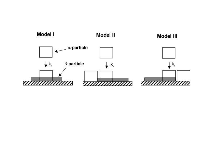


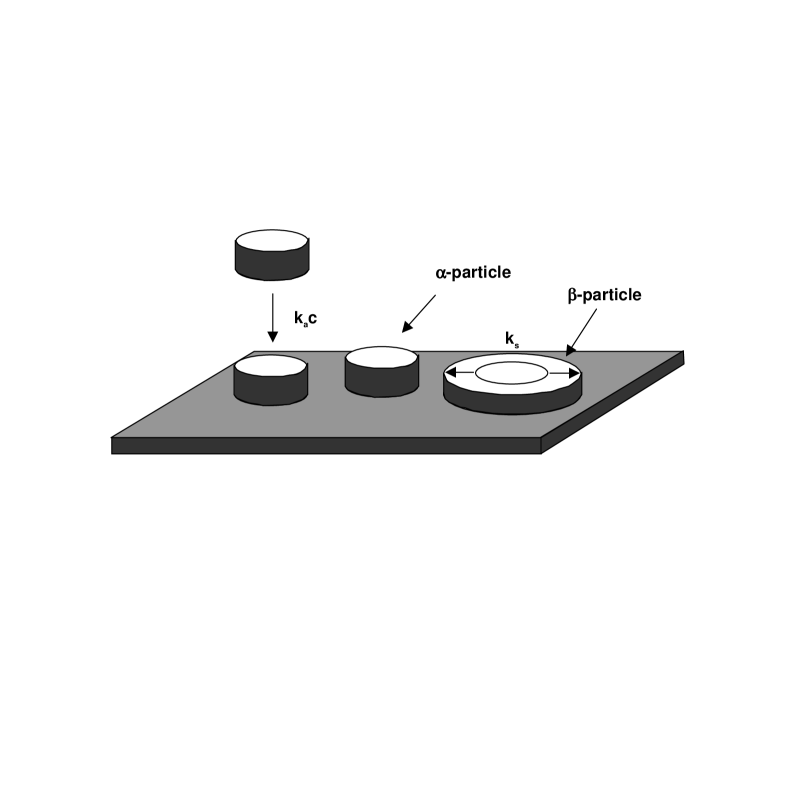

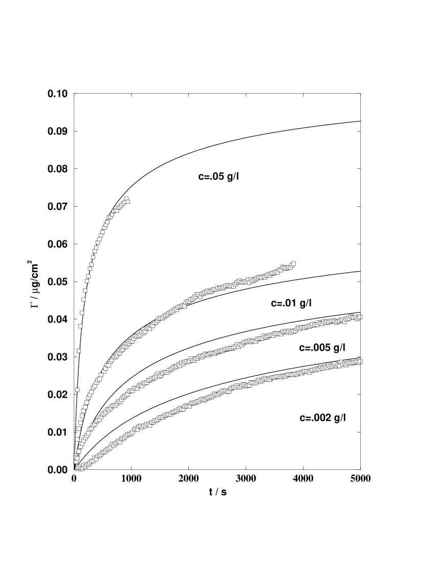


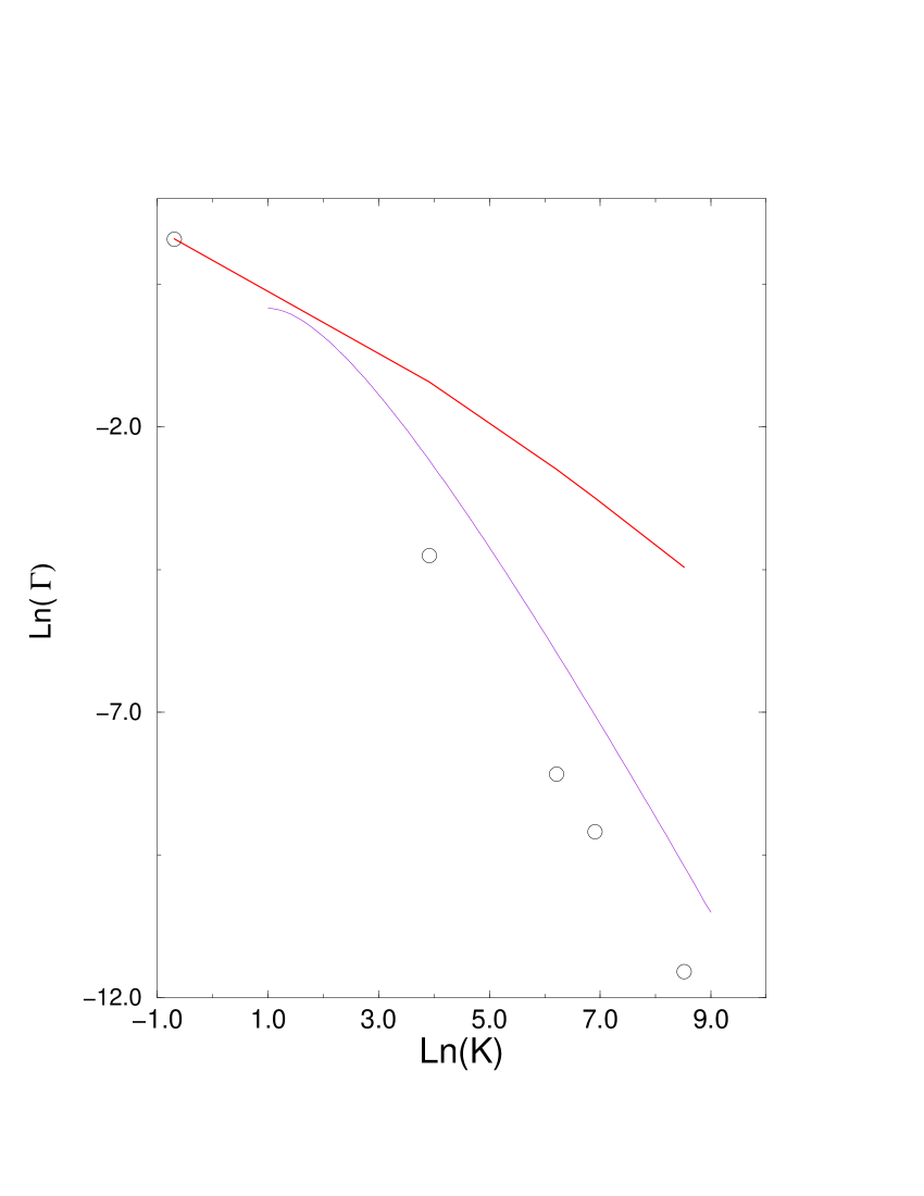
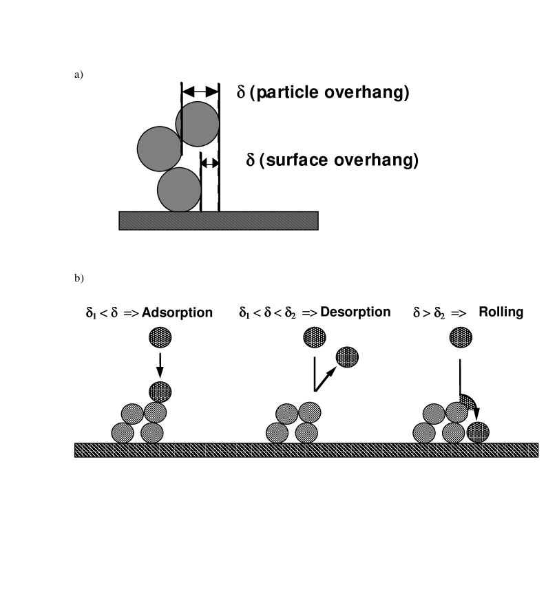

REFERENCES
- [1] J. Feder and I. Giaever, J. Colloid Interface Sci. 78, 144, (1980).
- [2] G.Y. Onoda and E.G. Liniger, Phys. Rev. Lett. 33, 715 (1986).
- [3] J.D. Andrade and V.L. Hlady, Adv. Polymer. Sci. 79, 1 (1986).
- [4] W. Norde, Adv. Colloid and Interface Sci. 25, 267 (1986).
- [5] J. J. Ramsden, Quart. Rev. of Biophysics 27, 1 (1993).
- [6] Z. Adamczyk, B. Siwer, M. Zembala, and P. Belouschek, Adv. in Colloid and Interface Sci. 48, 151 (1994).
- [7] M.C. Bartelt and V. Privman, Int. J. Mod. Phys. B 5, 2883 (1991).
- [8] J.W. Evans, Rev. Mod. Phys. 65, 1281 (1993).
- [9] A. Rényi, Sel. Trans. Math. Stat. Prob. 4, 205 (1963).
- [10] J.J. Gonzales, P.C. Hemmer and J.S. Hoye, Chem. Phys. 3, 228 (1974).
- [11] B. Bonnier, D. Boyer and P. Viot, J. Phys. A 27, 3671 (1994).
- [12] P. Schaaf and J. Talbot, Phys. Rev. Lett. 62, 175 (1989).
- [13] P. Schaaf and J. Talbot, J. Chem. Phys. 91, 4401 (1989).
- [14] G. Tarjus, P. Schaaf and J. Talbot, J. Stat. Phys. 63, 167 (1991).
- [15] J. Feder, J. Theor. Biol. 87, 237, (1980).
- [16] E.L. Hinrichsen, J. Feder, and T. Jøssang, J. Stat. Phys. 44, 793 (1986).
- [17] J. J. Ramsden, Phys. Rev. Lett., 71, 295 (1993).
- [18] Z. Adamczyk, M. Zembala, B. Siwek, and P. Warszýnski, J. Colloid Interface Sci. 140, 123 (1990);
- [19] Z. Adamczyk and P. Belouschek J. Colloid Interface Sci., 146, 123 (1991)
- [20] P. Wojtaszczyk, P. Schaaf, B. Senger, M. Zembala, J.C. Voegel J. Chem. Phys. 99, 7198 (1993).
- [21] B. Widom, J. Chem. Phys. 44, 3888 (1966).
- [22] M. Mézard, G. Parisi, and M.A. Virasoro, Spin Glass Theory and Beyond (World Scientific, Singapore, 1987).
- [23] J.A. Given, Phys. Rev. A45, 816 (1992).
- [24] Y. Pomeau, J. Phys. A13, L193 (1980).
- [25] R.H. Swendsen, Phys. Rev. A 24, 504 (1981).
- [26] G. Tarjus and J. Talbot Phys. Rev A 45, 4162 (1992).
- [27] J. Talbot, G.Tarjus, and P. Schaaf, Phys. Rev. A 40, 4808 (1989).
- [28] P. Viot and G. Tarjus, Europhys. Lett. 13, 295 (1990).
- [29] G. Tarjus and J. Talbot J. Phys. A24, L913 (1991).
- [30] J.P. Hansen and I.R. Mc Donald, Theory of Simple Liquids, Academic Press (1986).
- [31] Z. Adamczyk and P. Warszyński, Adv. Colloid and Interface Sci. 63, 41 (1996).
- [32] J. W. Evans, Phys. Rev. Lett. 62, 2642 (1989).
- [33] R. Dickman, J.-S. Wang, and I. Jensen, J. Chem. Phys. 94, 8252 (1991).
- [34] B. Bonnier, M. Hontebeyrie, and C. Meyers, Physica A198 1 (1993).
- [35] D. Boyer, G. Tarjus, P. Viot, and J. Talbot, J. Chem. Phys. 95, 1607 (1995).
- [36] I. Palasti, Publ. Math. Inst. Hung. Acad. Sci. 5, 353 (1960).
- [37] P. R. Van Tassel, G. Tarjus, and P. Viot, J. Chem. Phys. 106, 761 (1997).
- [38] S.M. Ricci, J. Talbot, and P. Viot, Mol. Simul. 13, 1 (1994).
- [39] J.S. Wang, Physica 254, 179 (1998) and references therein.
- [40] P. Schaaf, P. Déjardin, A. Johner, and A. Schmitt, Langmuir 8, 514 (1992).
- [41] M.J. Mura-Galelli, J.C. Voegel, S. Behr, E.F. Bres, and P. Schaaf, Proc. Natl. Acad. Sci., 88, 5557, (1991).
- [42] R. D. Vigil and R. M. Ziff, J. Chem. Phys. 91, 2599 (1989).
- [43] R. D. Vigil and R. M. Ziff, J. Chem. Phys. 93, 8270 (1990).
- [44] G. Tarjus, P. Viot, S. Ricci and J. Talbot, Mol. Phys. 73, 773 (1991).
- [45] G. Tarjus and P. Viot, Phys. Rev. Lett. 67, 1875 (1991).
- [46] S. Ricci, J. Talbot, G. Tarjus, and P. Viot, J. Chem. Phys. 97, 5219 (1992).
- [47] P. Viot, G. Tarjus, S. Ricci, and J. Talbot, Physica A 191, 248 (1992).
- [48] S.M. Ricci, J. Talbot, G. Tarjus, and P. Viot, J. Chem. Phys. 101, 9164 (1994).
- [49] T. Boublík, Mol. Phys., 29, 421 (1975).
- [50] D. Boyer, G. Tarjus, and P. Viot, Phys. Rev. E, 51, 1043 (1995).
- [51] R.M. Ziff and R.D. Vigill, J. Phys. A23 5103 (1990).
- [52] R.M. Ziff (unpublished).
- [53] J. Talbot and P.Schaaf, Phys. Rev. A 40, 422 1990.
- [54] P. Meakin and R. Jullien, Phys. Rev. A, 46, 2029 (1992).
- [55] P. Meakin and R. Jullien, Physica. A, 187, 475 (1992). (1992).
- [56] P. Schaaf, A. Johner, and J. Talbot, Phys. Rev. Lett. 66 1603 (1991).
- [57] F.J. Bafaluy, B. Senger, J.C. Voegel, and P. Schaaf, Phys. Rev. Lett 70, 623 (1993).
- [58] I. Pagonabarraga and J.M. Rubi, Phys. Rev. Lett. 73, 114 (1994).
- [59] P. Wojtaszczyk and J.B. Avalos, Phys. Rev. Lett. 80, 754 (1998).
- [60] B. Senger, J.-C Voegel, P. Schaaf, A. Johner, A. Schmitt, and J. Talbot, Phys. Rev. A 44, 6926 (1991).
- [61] B. Senger, P. Schaaf, J.-C Voegel, A. Johner, A. Schmitt,and J. Talbot, J. Chem. Phys 97, 3813 (1992).
- [62] G. Tarjus and P. Viot, Phys. Rev. Lett. 68, 2354 (1992).
- [63] F. J. Bafaluy, H. S. Choi, B. Senger and J. Talbot, Phys. Rev. E, 51, 5985 (1995).
- [64] B. Senger, J. Talbot, P. Schaaf, A. Schmitt and J.-C. Voegel, Europhys. Lett. 21, 135 (1993).
- [65] H.S.Choi and J.Talbot J. Stat. Phys. 92, 891 (1998).
- [66] J. Talbot and S. Ricci, Phys. Rev. Lett. 68, 958 (1992).
- [67] P. Viot, G. Tarjus, and J. Talbot, Phys. Rev. E 48, 480 (1993).
- [68] D. Boyer, G. Tarjus and P. Viot, J. Phys. A 29, 2309 (1996).
- [69] R. Jullien and P. Meakin, J. Phys.A 25, L189 (1992).
- [70] H.S. Choi, J. Talbot, G. Tarjus and P. Viot, J. Chem. Phys. 97, 4256 (1993).
- [71] G. Tarjus, P. Viot, H.S. Choi, and J. Talbot, Phys. Rev. E 49, 3239 (1994).
- [72] R.J. Baxter, J. Chem. Phys. 49, 2770 (1968).
- [73] A. P. Thompson and E.D. Glandt, Phys. Rev. A 46, 4639 (1992).
- [74] H.S. Choi, J. Talbot, G. Tarjus and P. Viot, Phys. Rev. E 51, 1353 (1995).
- [75] P. Wojtaszczyk, PhD thesis (Strasbourg University, 1995).50
- [76] G. Csúcs and J. J. Ramsden, J. Chem. Phys., 109, 779 (1998).
- [77] P. Schaaf, P. Dejardin, and A. Schmidt, Langmuir 3, 1131 (1987).
- [78] D. Boyer, G. Tarjus, J. Talbot, P. Van Tassel, and P. Viot, Phys. Rev. E 49, 5525 (1994).
- [79] P. R. Van Tassel, P. Viot, G. Tarjus, and J. Talbot, J. Chem. Phys. 101, 7064 (1994).
- [80] P. R. Van Tassel, J. Talbot, G. Tarjus, and P. Viot, Phys. Rev. E 53, 785 (1996).
- [81] P.R. Van Tassel, L. Guemouri, J.J. Ramsden, G. Tarjus, P. Viot, and J. Talbot, J. Colloid Interface Sci. 207, 317 (1998).
- [82] I. Pagonabarraga, J. Bafaluy, and J. M. Rubi, Phys, Rev. Lett. 75, 461 (1995).
- [83] P.R. Van Tassel, J. Talbot, P. Viot, and G. Tarjus, Phys. Rev. E 56, R1299, (1997).
- [84] P.R. Van Tassel, P. Viot, G. Tarjus, J.J. Ramsden, and J. Talbot, J. Chem. Phys., submitted (1999).
- [85] M.E. Soderquist and A.G. Walton, J. Colloid Interface Sci. 75, 386 (1980).
- [86] B.M. Morrisey, Ann. N.Y. Acad. Sci. 288, 50 (1977).
- [87] M. Wahlgren, T. Arnebrant, and I. Lundstrom, J. Colloid Interface Sci. 175, 506 (1995).
- [88] X. Jin, G. Tarjus and J. Talbot, J. Phys. A. 27, L195 (1994).
- [89] P. L. Krapivsky and E. Ben-Naim, J. Chem. Phys. 100, 6778, 1994.
- [90] E. Ben-Naim, J. B. Knight, E. R. Nowak, H. M. Jaeger, and S. R. Nagel, Physica D 123, 380 (1998).
- [91] Amy J. Kolan, Edmund R. Nowak, Alexei V. Tkachenko, cond-mat/9809434.
- [92] J. Talbot, G. Tarjus and P. Viot, J. Phys.A 32 2997 (1999).
- [93] E. R. Nowak, J. B. Knight, E. Ben-Naim, H. M. Jaeger and S. R. Nagel, Phys. Rev. E 57, 1971 (1998).
- [94] H. Reiss, H. L. Frisch and J. L. Lebowitz, J. Chem. Phys., 31, 369 (1959).
- [95] J. Talbot, J. Chem. Phys., 106, 4696 (1997).
- [96] A. P. Minton, Biophysical Journal, 76, 176 (1999).
- [97] X. Jin, Z. Ma, J. Talbot and N.-H. L. Wang, Langmuir, in press (1999).
- [98] C.B. Olson and J. Talbot, to be submitted.
- [99] M.A. Brusatori and P.R. Van Tassel, submitted to J. Colloid Int. Sci.
- [100] P.L. Krapivsky, J. Chem. Phys. 97, 2134 (1992).
- [101] M.C. Bartelt and J.W. Evans, J. Stat. Phys. 76, 867 (1994).
- [102] P. R. Van Tassel, and P. Viot, Europhys. Lett. 40, 293 (1997).
- [103] S. Yang, P.Viot and P.R. Van Tassel, Phys. Rev. E 58, 3324 (1998).
- [104] B.D. Lubachevsky, V. Privman, and S.C. Roy, Phys. Rev. E 48, 48 (1993).
- [105] J. Talbot, P. Schaaf, and G. Tarjus, Mol. Phys. 72 1397 (1991).
- [106] D.W. Cooper, Phys. Rev. A38 522 (1988).
- [107] B.J. Brosilow, R.M. Ziff, and R.D. Vigil, Phys. Rev. A 43, 631 (1991).
- [108] W.S. Jodrey and E.M. Tory, J. Stat. Comput. Simul. 10, 87 (1980).
- [109] D.W. Cooper, J. Appl. Prob. 26, 664 (1988).