Damage-Spreading in Self-Organized Critical Systems

Abstract

We study the behavior under perturbations of different versions of Bak-Sneppen (BS) model in $1\!+\!1$ dimension. We focus our attention on the damage-spreading features of the BS model with both random as well as deterministic updating, with sequential as well as parallel updating. In addition, we compute analytically the asymptotic plateau reached by the distance after the growing phase.

I Introduction

A great deal of evidence has been put forward in recent years for the appearance of power law statistics in nature: A wide variety of phenomena, from earthquakes [1, 2] to biological evolution [3, 4, 5, 6, 7], from surface growth [8] to fluid displacement in porous media [9], exhibit scale invariance in both space and time. To explain these all-pervading power-law tails, Bak, Tang, and Wiesenfeld introduced the concept of self-organized criticality (SOC) [10]. In a nutshell, SOC means that certain driven spatially extended systems evolve spontaneously towards a critical globally stationary dynamical state with no characteristic time or length scales [11]. This scale invariance implies that the correlation length in these systems is infinite and consequently a small (local) perturbation can produce a global (maybe even drastic) effect. This possibility leads naturally to the study of the sensitivity to perturbations in (self-organized) critical systems.

To study the propagation of local perturbations (damage spreading) one can borrow a technique from dynamical systems theory. Let us consider, for instance, two copies of the same dynamical system (let us say, for instance, a 1D map) , with slightly different initial conditions. By following the dynamics of both copies and studying the evolution in time of the “distance” $d(t)$ between them, it is possible to quantify the effect of the initial perturbation. Indeed, assuming that the distance $d(t)$ grows exponentially, and defining the Lyapunov exponent $\lambda$ via

$$D(t)=D_{0}\exp(\lambda\,t),$$ (1)

three different behaviors can be distinguished, corresponding to $\lambda$ being either positive, negative or zero. The case $\lambda>0$ corresponds to the so-called chaotic systems, where the extremely high sensibility to initial conditions leads to exponentially diverging trajectories on a strange (or chaotic) attractor. The case $\lambda<0$, instead, characterizes those systems in which the dynamics has an attractor and any initial perturbation is “washed out” with exponential rapidity.

The boundary case, $\lambda=0$, admits, in turn, a whole class of functions $D(t)$, namely

$$D(t)\,\sim\,t^{\alpha}\,.$$ (2)

where $\alpha$ is some exponent, characteristic of the system. In particular, $\alpha>0$ corresponds to weak sensitivity to initial conditions while $\alpha<0$ corresponds to weak insensitivity to initial conditions (as an example, the reader is referred to Refs. [12], where this analysis is performed for the logistic map at its critical point [13]).

Recently [14, 15, 16, 17], a similar analysis was performed on several versions of the Bak-Sneppen (BS) model [3]. Originally proposed to describe ecological evolution, this model has been paid a great deal of attention due to its simplicity and the fact that it exhibits self-organized criticality.

Schematically, the BS model is defined on a lattice where at each time-step one site is chosen, namely the one that fulfills a global constraint (minimum in some phase space). This site is defined as the active site. This dynamics leads to a non-Markovian process where the activity, i.e. the position on the lattice of the active site, jumps on the lattice following a (correlated) Lévy Walk. Its critical properties allow us to describe its behavior under perturbations via Eq. (2), with

$$\alpha\,=\,0.32\,.$$ (3)

In this paper we analyze in detail the behavior of different versions of the BS model. As we shall see, the particular stationary distribution of the variable does not play any role in the determination of the exponent $\alpha$ in Eq. (2). What matters is, instead, the kind of Lévy Walk involved and the strength of the correlations.

The paper is organized as follows. After a general description of our formalism in Sec. II, the BS model is discussed in Sec. III. In Sec. IV we analyze the behavior under perturbations of the deterministic BS model, introduced in [18, 19]. In Sec. V, we study the parallel version of it (PBS model), introduced not long ago by Sornette and Dornic [20]. We study two versions of it, namely the one with random updating and the one with logistic updating. We also present here a discussion of the differences and similarities between the BS and the PBS models. In Sec. VI we discuss the influence of changing the perturbation. Conclusions can be found in Sec. VII.

II General formalism: Damage-Spreading in the Ring

To illustrate our formalism, let us start by considering a lattice of $N$ sites on a one-dimensional ring $R_{1}$. To each site $j$ we assign a random number $f_{j}$, extracted from a uniform distribution between $0$ and $1$. We then consider a “replica” $R_{2}$, in which we introduce a perturbation by exchanging the positions of the values of $f_{k_{1}}$ and $f_{k_{2}}$. We define as active the sites $k_{1}$ in $R_{1}$ and (the randomly chosen site) $k_{2}$ in $R_{2}$, namely those sites at which we have the same value of $f$. It is clear that, from a statistical point of view, both system $R_{1}$ and replica $R_{2}$ are described by the same distribution function. The prescription just introduced corresponds, in a suitably defined phase space, to a small difference in the initial conditions between $R_{1}$ and $R_{2}$ (see Eq. (8) below). Moreover, this procedure of finding an active site and exchanging its position with another site taken at random along the lattice, corresponds exactly to the one proposed in [14] for the Bak-Sneppen model (other definitions for the initial perturbation are considered elsewhere [16]). The dynamics on the ring(s) is defined as follows. At each time-step, an integer random number $x$ between $1$ and $N$ is chosen. Bearing in mind that our rings have periodic boundary conditions, the positions of the new active sites at time $t+1$ is then given by

$$k_{1}(t+1) = k_{1}(t)+x$$ (4)

$$k_{2}(t+1) = k_{2}(t)+x$$ (5)

on the rings $R_{1}$ and $R_{2}$ respectively. On these active sites, the value of the variables $f$ is changed, assigning to both of them the same random number (this corresponds to the choice of the same sequence of random numbers in [14] or to the same thermal noise in usual damage spreading calculations [21]).

As both system $R_{1}$ and replica $R_{2}$ evolve, we compute the Hamming distance, namely

$$D(t)\,=\,\frac{1}{N}\sum_{j=1}^{N}\,|f_{j}^{1}-f_{j}^{2}|\,.$$ (6)

Since this quantity has strong fluctuations, we will consider the average $\langle D(t)\rangle$, over realizations. In particular, at $t=1$, the average (initial) distance $\langle D(1)\rangle$ can be obtained from Eq. (6),

$$\langle D(1)\rangle\,=\,\frac{2}{N}\int_{0}^{1}\,df_{1}df_{2}\,\eta_{1}(f^{1})\eta_{2}(f^{2})\,|f^{1}-f^{2}|,$$ (7)

where $\eta_{i}$ is the distribution function (at $t=1$) for the variable $f^{i}\in R_{i}$. In this toy model, both distributions $\eta_{i}(f)$ are the same, namely a uniform distribution in $f^{i}\in R_{i}$. A simple computation yields

$$\langle D(1)\rangle=\frac{2}{3N}\,.$$ (8)

Applying a similar procedure, one can verify that for $1\!\ll\!t\!\ll\!N$ the distance grows linearly. Indeed, let us define $\sigma(t)$ as the averaged number of different sites covered in one copy of the system at time $1\!\ll\!t\!\ll\!N$. Then, at time $t$ only $\sigma(t)$ sites have been changed and these are the only ones that contribute to distance. From this consideration it follows that

$$\langle D(t)\rangle\,=\,\langle D(1)\rangle\,\sigma(t)\,,$$ (9)

where the fact that both replica contribute to the distance on the same footing is taken into account in Eq. (8). In the case of the ring, if $N\!\gg\!1$ and $1\!\ll\!t\!\ll\!N$ the system will always choose a new site at each time-step, and therefore $\sigma(t)\sim t$ (note that, in the 1D case for this dynamics, this is the fastest possible growth of $\langle D(t)\rangle$). This behavior stops at times $t\sim N$ where a crossover to a saturation regime appears. Clearly, after $t\propto N$ time steps each site of the lattice has been covered at least once. For $t\gg N$, almost all the lattice sites have been covered and the two strings are made of the same random numbers shifted by $k_{2}-k_{1}$. Thus, the distance reaches a plateau, independent on the size $N$ of the system, given by

$$\langle D(t\to\infty)\rangle\,=\,\int_{0}^{1}df^{1}df^{2}\,\rho_{1}(f^{1})\rho_{2}(f^{2})\,|f^{1}-f^{2}|\,,$$ (10)

where $\rho_{i}$ is the normalized distribution function (at $t=\infty$) for the variable $f^{i}\in R_{i}$. In Eq. (10), for the particular case of the ring the distributions in the integral are given by $\rho_{i}=\eta_{i}$. Applying Eq. (10) to $R_{1}$ and $R_{2}$ we finally obtain

$$\lim_{t\to\infty}\,\langle D(t)\rangle\,=\,\frac{1}{3}\,.$$ (11)

Note that the same result can be obtained from Eqs. (8,9) once $\sigma=N$ is inserted. To have an initial distance independent of the lattice size, we consider the ratio $\langle D(t)\rangle/\langle D(1)\rangle$. For this ratio, however, the value of the plateau depends linearly on $N$, i.e.

$$\frac{\langle D(\infty)\rangle}{\langle D(1)\rangle}=\frac{N}{2}.$$ (12)

In Fig. 1 we show the evolution in time of the ratio $\frac{\langle D(t)\rangle}{\langle D(1)\rangle}$, averaged over many realizations, for different lattice sizes. The plateau reached for $t\to\infty$ depends on $N$ according to Eq. (12). The exponent $\alpha=1$ obtained for this case from Eq. (9) can also be numerically obtained with great accuracy. From a physical point of view, this power law behavior originates in the ability of the system to cover the lattice. As we have seen, the activity can jump anywhere on the lattice with probability $1/N$. Thus the number of sites $j$ with the same $f_{j}$ decreases linearly with time and $\langle D(t)\rangle$ increases linearly with time. As a consequence, the time $\tau$ needed to reach the plateau scales with the lattice size as $\tau\sim N$.

Keeping in mind our goal of modeling the behavior of the BS model, let us now consider the case of Lévy-Walk type activity jumps along the lattice. More precisely, the length $x$ of any jump is extracted from a power law distribution function, namely

$$P(x)\,=\,(\beta-1)\,x^{-\beta}\,,$$ (13)

where the minimum jump is $x=1$ and the jump can be to the left or to the right.

As before, the position of the new active site is obtained by jumping $x$ sites from the present one, i.e. the position of the new active site will be given by Eqs. (4,5), where now each copy of the system has its own $x$. Thus, the values of $x$ are un-correlated between the two copies of the system. The new values of $f$ assigned to the active sites are the same. This choice results in a different behavior at the saturation regime.

In the Random Walk limit, $\beta\gg 1$ in Eq. (13), the distance Eq. (7), can be easily computed by considering Eq. (9) together with the fact that $\sigma\sim t^{1/2}$ . This calculation yields

$$\langle D(t)\rangle\,\sim\,t^{1/2}\,.$$ (14)

In the general case $\beta>1$, there is still a power law growth of the distance (6) for intermediate times $1\ll t\ll N$. The exponent in Eq. (2) can be obtained using the fact that the mean-square distance $\sigma^{2}$ covered by a Lévy Walk behaves like

$$\sigma^{2}(t) \sim \left\{\begin{array}[]{lr}t^{2}&(1<\beta\leq 2)\\ t^{4-\beta}&(2<\beta<3)\\ t\log t&(\beta=3)\\ t&(\beta>3)\end{array}\right.\,,$$ (19)

in the long-time limit. As a consequence, one can also compute the so-called dynamical exponent $z$ defined through $\tau\sim N^{z}$ where $\tau$ is the time needed for the distance (actually the ratio $\frac{\langle D(t)\rangle}{\langle D(1)\rangle}$) to reach the plateau. This time is given by the time needed to cover all the lattice sites, if finite size effects are not counted in. Comparison between Eqs. (2,9,19) yields $z=\frac{1}{\alpha}$.

In this simple model we have excluded any kind of correlation between the values of $x$ extracted from Eq. (13) and between the two replicas at $t=1$. Indeed, the dynamics is given by a generalized random walk and therefore the power-law behavior of the growth is not related to the statistical properties of the system. This is in fact the idea behind our toy model: We use it as a “black box”, not knowing what happens inside, we are only able to observe a Lévy Walk behavior of the activity. Our model is, by conception, a trivial system that has as only purpose that of showing what are the consequences, in the context of damage-spreading, of a power-law behavior of the activity like the one observed in the Bak-Sneppen model.

As we shall see in the next section, the non-trivial properties of the self organized critical systems are hidden in the value of the exponent $\alpha$ in Eq. (2). Furthermore, the averaging procedure leading from Eq. (6) to Eq. (9) plays a very important role in these non-trivial systems.

Before moving onto the analysis of the BS model, let us discuss in more detail which terms are contributing to the computation of $\langle D(t)\rangle$ via Eq. (9). In the ring, we have defined $\langle D(t)\rangle$ by considering the behavior of $\sigma(t)$, which is a physical quantity related only to the behavior of the activity in one single system. In general, considering that the two replica might be correlated, we need to update Eq. (9) to

$$\langle D(t)\rangle\,=\,\langle D(1)\rangle\,{\bar{n}}_{cov}(t)\,,$$ (20)

where ${\bar{n}}_{cov}(t)$ is the average number of different sites covered by both system and copy. More precisely, suppose that at time $t$, the activity has covered $\sigma_{1}$ and $\sigma_{2}$ different sites in $R_{1}$ and $R_{2}$ respectively. Then, the function ${\bar{n}}_{cov}(t)$ is given by

$${\bar{n}}_{cov}(t)\,=\,\langle\sigma_{1}+\sigma_{2}-\sigma_{1,2}\rangle\,.$$ (21)

where $\sigma_{1,2}$ represents the number of sites covered in both systems (i.e. the covering overlap between system and copy). In the case of the ring, for large $N$ and $t\ll N$, the overlap on the rhs of Eq. (21) is empty ($\sigma_{1,2}\equiv 0$) and Eq. (20) reduces to Eq. (9). In the case of the Bak-Sneppen model instead, this intersection cannot be empty even in the thermodynamic limit. As a consequence, the exponents predicted from Eq. (19) have to be considered as an upper bound for those observables in systems with non-trivial correlations.

III The Bak-Sneppen Model

As mentioned above, in its simplest version the BS model describes an ecosystem as a collection of $N$ species on a one dimensional lattice. To each species corresponds a fitness described by a number $f$ between $0$ and $1$. For simplicity, one considers periodic boundary conditions. The initial state of the system is defined by assigning to each site $j$ a random fitness $f_{j}$ chosen from a uniform distribution. The dynamics proceeds in three basic steps:

1. Find the site with the absolute minimum fitness on the lattice (the active site) and its two nearest neighbors.

2. Update the values of their fitnesses by assigning to them new random numbers from a uniform distribution.

3. Return to step 1.

After an initial transient that will be of no interest to us here, a non-trivial critical state is reached. This critical state, characterized by its statistical properties, can be understood as the fluctuating balance between two competing “forces”. Indeed, while the random assignation of the values, together with the coupling, acts as an entropic disorder, the choice of the minimum acts as an ordering force. As a result of this competition, at the stationary state the majority of the $f_{j}$ have values above a certain threshold $f_{c}=0.66702(1)$ [3]. In other words, the distribution function of the $f_{j}$’s can be asymptotically approximated by

$$\eta_{1}(f)\,=\,\frac{1}{1-f_{c}}\,\Theta(f-f_{c})\,,$$ (22)

where $\Theta(f)$ is the Heaviside function. Only a few will be below $f_{c}$, namely those belonging to the running avalanche (see [3, 22] for a detailed discussion). Proceeding by analogy with the previous cases, once the system is at the critical state, we produce two identical copies $B_{1}$ and $B_{2}$ and find the minimum (the active site). Then, in $B_{2}$ we swap the value of the minimum fitness with the fitness of some other site chosen at random (note that if $N$ is big enough, the fitness in the other site will certainly be above threshold). After that, the evolution of the Hamming distance given by Eq. (6) is studied. In the evolution of both system and copy the same random numbers are used. Here, the length of the jumps in the position of the active site follows a power-law distribution given by Eq. (13) with $\beta\sim 3.23$ [3]. At variance with the case of the ring discussed above, we cannot expect the behavior shown in Eqs. (9) and (19). Indeed, in the BS model the jumps posses strong spatial correlations, with large probability of returning to sites already covered in previous time-steps. As a consequence, the behavior of the number of different sites covered in one single system cannot be given by Eq. (19) but leads to $\sigma(t)\sim t^{\mu}$ for $t\gg 1$ [3], with $\mu=0.4114\pm 0.0020$ [23]. Moreover, as we consider the two copies $B_{1}$ and $B_{2}$ we immediately realize that the two systems are also strongly correlated and consequently one obtains an even smaller exponent leading to

$$\langle D(t)\rangle\,\sim\,t^{\alpha=0.32}\,.$$ (23)

As we mentioned at the end of Sec. II, the behavior of Eq. (23) can be understood in the framework of Eq. (20). In fact, the decrease in the value of $\alpha$ is given by the appearance of $\sigma_{1,2}\neq 0$ in Eq. (20).

Indeed, the fact that we are using the same sequence of random numbers implies that, if the system is big enough the absolute minimum in one system is the absolute minimum also in the copy. Therefore, if the absolute minimum is among those sites which have not yet been covered by the activity, the three terms in the rhs of Eq. (21) will have the same behavior. If the minimum is instead one of the newer values put in the system after perturbation, its position on the lattice may be different in the two replica but the three functions in the rhs of Eq. (21) grow slowly or even do not grow at all. This observation is confirmed by the irregular behavior of $D(t)$ in just one single realization. In fact, it is the averaging procedure the one that produces finally a smooth curve. It should be noted that, as it is clear from its definition, the behavior of the intersection is strongly correlated to the behavior of the other two sets and therefore the average in the rhs cannot be split into the sum of the independent averages. As a consequence we should expect a smaller exponent with respect to the one obtained for $\sigma(t)$.

The initial distance can be computed using Eq. (8). To do that we need the distribution function of the value of the minimum. Extensive numerical simulations indicate that this distribution can be approximated by

$$\eta_{2}(f)\,=\,\left(3-\frac{9}{2}\,f\right)\,\Theta(\frac{2}{3}-f)\,,$$ (24)

where the threshold has been put equal to $2/3$. Inserting (24) and (22) in Eq. (8) we obtain $\langle D(1)\rangle\sim\frac{11}{9N}$. Since $\langle D(t\to\infty)\rangle$ takes into account all sites on the same footing, this saturation value can be obtained from Eq. (10) with $\rho_{1}=\rho_{2}=\eta_{1}$. The distribution $\eta_{1}$ comes from Eq. (22), and the saturation value is $\langle D(t\to\infty)\rangle\sim\frac{1}{9}$. Therefore, as in the case of the ring, the saturation value does not depend on the size of the system while the initial distance does. Thus, the normalized distance reaches a plateau that must scale with $N$, as our numerical simulations show (see Fig. 2).

Coming back to the dynamical exponent $z$, we find that it still follows the prediction $z=1/\alpha$ as in the case of the ring. For the BS model one obtains, following the above described prescription, $z\sim 3.12$, instead of $z\sim 1.6$ determined in [14]. This value $z\sim 3.12$ coincides reasonably well with the one obtained from the collapse plot (Fig. 3). The reason for the discrepancy between our results and those presented in [14] can be traced back to the effects of time-rescaling on the (normalized) growth function. Indeed, let us assume we use a different time-scale, and consider the case in which we make a measure of $D(t)$ every $\nu$ time-steps (instead of every time-step), where $\nu$ is distributed according to a certain function $P(\nu)$. The rescaled distance $\tilde{D}(t)$ will be given by

$$\tilde{D}(t)\,=\,\int\mbox{d}\nu\,P(\nu)\,D\left((t-1)\langle\nu\rangle\,+\nu\right)\,,$$ (25)

where $\langle\nu\rangle=\int\mbox{d}\nu\nu P(\nu)$ is the average number of time-steps between two consecutive measurements. The choice made in [14] corresponds to $P(\nu)=\delta(\nu-N)$. It is easy to see that, in this case, the growth exponent for $\tilde{D}(t)$ is still $\alpha$, but the measured dynamical exponent is given by $1/\alpha-1$. In principle, one could imagine more complicated distributions $P(\nu)$ for the measuring time. In particular, if $P(\nu)$ did not have a finite first moment (as would be the case, for instance, if $P(\nu)$ corresponded to the avalanche distribution) Eq. (25) would yield $\tilde{D}(2)\approx N$, i.e. the rescaled distance would saturate almost immediately [24].

In order to study the size dependence of $\alpha$ we have performed a set of measurements for different system sizes and then extrapolated the value of $\alpha$ to infinite size. We get an asymptotic value $\alpha_{asym}=0.40(1)$ (see Fig. 4).

At this point, it is worth discussing what happens in higher dimensions. The high-dimensional Bak-Sneppen model has been extensively studied in [25], where the behavior of the exponent $\mu$ for the growth of the quantity $\sigma(t)$ has been computed until the mean-field regime $\mu=1$ has been reached. In the framework of the damage-spreading, taking into account the correlations as discussed above, one expects the exponent $\alpha$ to follow a similar pattern, reaching the value $\alpha=1$ in the mean-field case. These mean-field results can also be obtained in the random-neighbors case [26]. However, from the point of view of damage spreading, the random nearest neighbor case presents a complication. There is an ambiguity in the choice of the neighbors. Indeed, their absolute positions on the lattice should be either the same in the two copies of the system or taken at random in an uncorrelated fashion. In both cases, each one of the two copies will behave normally, but the behavior of the distance will be completely different. Indeed, in the first case the distance between the two systems will never grow, while in the latter case the behavior of the distance resembles that of the ring with uniformly distributed jumps.

IV BS Model without noise

Through the use of different maps (chaotic as well as non-chaotic), it was shown [18, 19] that the random updating is not a necessary requirement to have SOC. Moreover, as long as the updating rule is chaotic the system does not change the universality class, i.e. all the exponents are the same as in the case of random updating. This means that the system is able to self-organize at a higher level: It takes into account the temporal correlation (or the average time spent in every site) by increasing the threshold, so as to have the same statistical properties [18, 19]. As a consequence, all equations and relations derived for the original BS model are still valid for all the cases with chaotic updating. The stationary distribution of the fitnesses, on the other hand, follows a different pattern. Indeed, the position of the threshold as well as the exact shape of the stationary distribution depends on the actual form of the updating rule.

To calculate the value of $\langle D(1)\rangle$ one needs to specify the nature of the perturbation. Using the same methods as in the random updating case, i.e. to swap the position of the minimum in $B_{2}$ with any site taken at random, at $t=1$, the average (initial) distance $\langle D(1)\rangle$ can be obtained from Eq. (7), where $\eta_{i}$ is the distribution function (at $t=1$) for the variable $f^{i}\in B_{i}$.

When one considers the chaotic updating, Eqs. (7,10) are still valid. The only difference is that one needs to find the stationary distributions that correspond to the actual map. For instance, for the tent map as well as for the Bernoulli map the distribution coincides with that of the random updating (except for the value of the threshold in the Bernoulli case) [18, 19]. As an example, we substitute the random updating with the logistic map

$$f_{i}(t+1)=bf_{i}(t)(1-f_{i}(t))\,,$$ (26)

where $i$ runs over the minimum and its nearest neighbors and $b$ is a parameter (that we set to the value $4$ which is at the threshold of the chaotic phase). Inserting the estimated distributions obtained in [18, 19] one obtains as first approximation $D_{asym}\sim 0.087$ and the same exponent $\alpha$ as in the random updating.

In Fig. 5 one can see the evolution of the distance for the case of a Bak-Sneppen model with random and logistic updating, using the perturbation defined in [14] (flipping of the minimum fitness with another fitness chosen at random). Simulations with other chaotic maps give the same exponents too: This reflects the observed fact that chaotic maps do not change the universality class of the model [18, 19]. In the inset we show the scaling of $ND_{asym}(N)$ versus $N$ for both random and logistic updating. A linear fit gives as estimation of the plateau $D_{asym}=0.112(5)$ for random updating and $D_{asym}=0.088(5)$ for logistic updating, in good agreement with our analytic estimate.

V parallel BS model

The $d$-dimensional parallel version of the BS model (PBS) [20], where parallel updating has been introduced, has been found to have an exact mapping onto $2d$ Directed Percolation. In fact, the avalanche time distribution in the PBS model is equivalent to the cluster distribution in DP and the threshold for PBS is equivalent to the critical probability in DP.

The dynamics in the PBS is different from the one in the (usual) Bak-Sneppen model due to the introduction of parallel updating:

1. Find the site with the absolute minimum fitness $f_{min}$ on the lattice (the active site) and its two nearest neighbors.

2. Update the values of their fitness by assigning to them new random numbers from a uniform distribution.

3. Search for all sites on the lattice with fitness $f<f_{min}$ and update them together with their nearest neighbors. Repeat the search until there are no sites left with $f<f_{min}$.

4. Return to step 1.

The difference between the PBS model and the original BS model lies in step 3. In the extremal version, once the minimum and its nearest neighbors are updated one looks for the new minimum, and consequently the number of updated sites per time step, $U_{t}$, is constant ($U_{t}\equiv 3$). In the parallel version, instead, this number will follow a complex temporal evolution during an avalanche with, in general, $U_{t}\geq 3$. In fact, the distribution of the number of updated sites per time step (inside an avalanche) shows a nearly flat distribution, with a upper cutoff, whose value is comparable with the system size [17]. Due to this saturation, one observes that $D(t)$ grows in time faster than in the BS case and that finite size effects are also much stronger.

Since the disorder is stronger in the parallel version ($U_{t}\geq 3$), one expects the equilibrium point to be displaced towards the completely disordered value. In fact, for the PBS model, $f_{c}\approx 0.5371(1)$ [20]. This results can be obtained both numerically and analytically by mapping the model onto directed percolation.

To study the behavior under perturbations of the PBS model, we follow the same procedure as for the extremal case. We produce two identical copies $B_{1}$ and $B_{2}$ of the system of size $N$ in the critical state, and find the minimum (the active site). Then, we introduce a slight perturbation in $B_{2}$ and follow the evolution of the Hamming distance Eq. (6) in time. Since this quantity has strong fluctuations, we consider the average $\langle D(t)\rangle$ over different realizations of the initial values of the $f_{j}$. In particular all the simulations presented here, are the result of averaging over $10^{2}$ realizations. The simulations are performed with both random and deterministic (logistic) updating rules. Let us begin by discussing the results obtained for random updating. As mentioned above, $D(t)$ may depend on the internal correlation of the system and on the correlations between the two copies. In the $1D$ BS model, due to the choice of unit of time, which allows only a number O(1) of sites to be updated, the growth rate must give an exponent $\alpha\!<\!1$ and stop at a certain time $\tau\sim N^{z}$, at which a crossover to a saturation regime appears.

In the PBS case, too, $D(t)$ reaches, after an initial power law growth (as in the BS case), a well defined plateau (see Fig. 6). However, due to the faster parallel dynamics, the value of the exponent $\alpha$ is found to be larger than the one for the the extremal non-parallel case, as shown in Table I. Moreover, there seem not to be dependence of the exponent $\alpha$ on the system size $N$. Notice that our exponent differs from the one obtained in [27] for the Domany-Kinzel model in the context of DP, onto which the PBS can be mapped. This discrepancy is due to the choice of time-scale for the measure of the distance. Indeed, in the Domany-Kinzel model case only one active (occupied) site per time step can be updated, together with its neighbor, thus resulting in a dilated time scale with respect to the study presented here. Thus, in order to compare the two models one has to establish the relationship between the two time-scales. This is not easy to realize for the Hamming distance. In fact, according to this interpretation, equal times for the two copies on the Monte-Carlo parallel time-scale are not equal times on the DP-like time-scale. To circumvent this problem, we realized a set of PBS simulations (with system size $N=2000$) for a single copy, computing at every Monte-Carlo (parallel) time step $\delta t=1$ the number $n_{act}(t)$ of sites below threshold (which is itself time-dependent). This defines the temporal increment for the DP-like time scale $\delta t_{DP}=\delta t\cdot n_{act}(t)=n_{act}(t)$. The effective DP time at the MC step $t$ is thus connected to the effective time at MC step $t-1$ by the relation:

$$t_{DP}(t)=t_{DP}(t-1)+n_{act}(t).$$ (27)

Then, we mediated over different realizations of the dynamics, obtaining the scaling of the effective DP time with the MC time of the simulation. The result, shown in Fig. 7, is that $t_{DP}\sim t^{\zeta}$ with $\zeta=1.41(2)$. From this, if we assume that $t_{DP}$ is the equivalent of the DP time-scale for PBS, we can combine the scaling law for $D(t)$ and that for $t_{DP}$ to get the effective scaling exponent $\alpha^{*}$ for the Hamming distance with respect to the DP time-scale $t_{DP}$:

$$\alpha^{*}=\frac{\alpha}{\zeta}=\frac{0.47}{1.41}=0.33(1).$$ (28)

This value is quite near to the DP exponent $\alpha_{DP}=0.314(1)$ [27].

At any given time step $t$ during an avalanche, the average growth of $D(t)$ is connected to the mean number of sites $\sigma(t)$ covered by the activity in each system according to Eq. (9). In Fig. 8, $\sigma(t)$ exhibits a power law behavior, $\sigma(t)\sim t^{\mu}$. The values of the scaling exponent $\mu$ at different sizes $N$ are always bigger than the corresponding values of the exponents for the Hamming distance (Tab. I). This is expected since the correlations between the two copies in $D(t)$, if present, can only decrease the value of $\alpha$ with respect to $\mu$ [15]. The asymptotic value of the Hamming distance shows quite a strong and persistent dependence on the system size $N$ and converges to an asymptotic value only logarithmically in $N$ (see inset of Fig. 6). Then, in order to get the real value of the plateau, one has to go to the thermodynamic limit $N=\infty$, once the plateau has been reached. This is realized by a logarithmic extrapolation of the data for different sizes. The value of this plateau can be obtained in terms of the asymptotic stationary fitness distribution $\rho(f)$ from Eq. (10) where $\rho_{i}(f)$ is the normalized distribution function (at $t=\infty$) for the variables $f^{i}\in B_{i}$, at a given system size $N$. The dependence of the plateau $D_{asym}(N)$ on $N$ must then be related to the shape of the stationary fitness distribution. The fitness distribution has, in fact, a flat tail below the threshold $f_{c}$, which disappears only logarithmically in $N$ as the system size is increased. In the limit $N\to\infty$ the distribution $\rho_{i}(f)$ is given by Eq. (22) with $f_{c}=0.5371$. By substituting the distribution $\rho_{i}$ thus obtained into Eq. (10) we get $D_{asym}(N=\infty)=D_{asym}=0.1543$ as estimation of the plateau in the thermodynamic limit. Turning back our attention to Fig. 6, one can see that this result is consistent with the extrapolated numerical value $D_{asym}\sim 0.14(2)$.

We have also performed a similar analysis for the PBS model with a deterministic updating, in which the new fitnesses are obtained by iterating the logistic map, namely

$$f_{i}(t+1)=bf_{i}(t)(1-f_{i}(t)),$$ (29)

where $f_{i}(t)$ is the fitness of site $i$ at time $t$, and $b$ is a parameter set to the value $4$ [18, 19]. We observe the same qualitative behavior for all the quantities studied in the random updating case. The fitness distribution is however different since it is influenced by the invariant measure of the map, as pointed out in [18, 19]. In the present case, the fitness distribution is strongly picked around $f=0$ and around $f=1$, for finite sizes $N$. The distribution is of course not symmetric and in the large $N$ limit, all the $f_{j}$ are above a threshold $f_{c}=0.55(1)$ [28]. The value of the plateau $D_{asym}$ converges, in the limit $N\to\infty$, to $D_{asym}\sim 0.15(2)$. By inserting the fitness distributions thus obtained in Eq. (10), we obtain an analytic estimation, $D_{asym}=0.1556$, that is indeed very close to the random updating analytical value, and in agreement with our numerical results. This is reasonable, since the threshold of the parallel BS with deterministic rule is very near the threshold of the random updating case. Although we performed, for the computation of the plateau, simulations up to system size $N=8000$, the need of a logarithmic extrapolation towards $N=\infty$ prevents us from obtaining a precise numerical estimation of the plateau. The values of the exponents $\alpha$ and $\mu$ show no substantial differences with respect to the random updating case, as is the case for the extremal BS model [16], thus confirming the robustness of $\alpha$ with respect to different updating rules.

VI on the initial perturbations

One point remains, however, that needs to be studied. The definition of the initial perturbation in the replica in [14] is too restrictive. In fact, by considering as initial perturbation

$$\tilde{f}_{i}=f_{i}+\epsilon g_{i}\,,$$ (30)

where $\epsilon$ is a small positive number, we can take several choices for $g_{i}$ without altering the exponent $\alpha$. We considered four different implementations of $g_{i}$:

  (a)

$g_{i}=\psi(t)$ where $\psi(t)$ is a random number between 0 and 1.

  (b)

$g_{i}=\psi(t)$ where $\psi(t)$ is a random number between -1/2 and 1/2.

  (c)

$g_{i}=\psi(t)$ for $i$ corresponding to the minimum and zero otherwise.

  (d)

$g_{i}=constant=1$ for all sites.

This kind of perturbation allows us to tune the initial mean distance $D(t)$, to any arbitrarily small value depending on $\epsilon$ in Eq. (30) (contrary on the flipping introduced in [14], which gives a fixed, size dependent, mean initial distance). In case (d), for example, (which is the case we will use in the analysis below) the initial distance is $D(1)=\epsilon$, independent on $N$, and the plateau will be independent on $N$ too. This characteristic of the global perturbation is useful to explore some properties of the model with deterministic updating and is more in line with the standard techniques of damage spreading problems.

We have performed the analysis with the prescription (30) also in the case in which the model has a deterministic microscopic rule, like an updating with the logistic map. In this case, the numbers in each replica will not be the same since the map will be applied on different numbers. In Fig. 9 we show the behavior of $D(t)$ for random and logistic updating, where we used perturbation (30) with the implementation (d). The exponent does not change: In both cases a value of $\alpha$ around the value $0.32$ found in [14] is obtained. The plateau of $ND(t)$ (we computed $ND(t)$ to reduce statistical fluctuations) for the case of global perturbation, scales linearly with the system size $N$, as shown in the inset of Fig. 7, with a slope $a=D_{asym}=0.114(5)$ and $a=D_{asym}=0.089(5)$ respectively for random updating and logistic updating. The good agreement with the rough analytic estimate obtained above and with numerical results for the flipping shows that the value of the plateau, too, does not depend on the kind of perturbation applied. Consequently, the distance $D(t)$ has a plateau $D_{asym}$ independent on the size, as it happens with the flipping. These results do not change if we use the implementations $(a),(b),(c)$ of the perturbation (30).

The case of the logistic map with perturbation (30) is particularly interesting from a different point of view. Since the map is chaotic, one could expect that on small scale distances ($D(t)\ll 1/N$) the chaoticity of the maps dominates and the distance of the two copies grows exponentially. For bigger distances instead, the dynamics is dominated by the damage spreading (and thus the critical properties of the BS model) and the distance grows as a power law. This is exactly what we find numerically. In Fig. 10 we show numerical simulations of the BS model with deterministic updating with the logistic map (with parameter value $4$) and random perturbation, for different system sizes and initial distances. The distance $D(t)$ has an initial exponentially growing phase with a Lyapunov exponent $\lambda=0.49(1)$. This Lyapunov exponent is smaller than the Lyapunov exponent of a single logistic map with $b=4$, which actually is $log2=0.693147...$. Indeed, the microscopic dynamical rule of the system changes the values of the minimum fitness and its nearest neighbors, and the Lyapunov exponent we measure arises from the interaction between the three maps applied to the three different numbers.

VII Conclusions

We have shown that the power-law behavior of the distance Eq. (2) has its origins in the behavior of the mean-squared distance covered by the activity. The first consequence is that $\alpha\leq 1$. The second is that the internal correlations of the jumps, governed by Eq. (13), and the strong correlations between the two copies, can severely slow down the growth of $\langle D(t)\rangle$, thus leading to smaller exponents with respect to the ones predicted in Eq. (19). Since an analytic derivation of the exponents characterizing the critical properties of the BS model is yet to be found, we had to base our work on numerical results. Nevertheless, by rewriting Eq. (2) into the more appropriate form given by Eqs. (20-21), we have been able to study the mechanisms leading to it. In the framework of these equations the occurrence of the plateau can be also easily understood and we have computed its value.

Our theory assumes that neither in the BS case nor in the case of the ring will the distribution of the variables $f$ change during the measurement of $\langle D(t)\rangle$ (we exclude the transient).

Moreover, we have studied the characteristics of damage spreading in a parallel version of the Bak-Sneppen model, and compared them to those of the extremal version. In general, the PBS model exhibits a faster evolution towards a stationary state, which is strongly dependent on the system size $N$.

Finally we have confirmed the picture presented in [19] according to which the application of deterministic (chaotic) maps does not change the universality class of the model. Furthermore, we have shown here that the analysis attempted in [14] and [15] is independent of the microscopic details of the system, and of the prescription of the initial perturbation. This of particular importance if one looks at these results within the framework of standard damage-spreading. The possibility to apply this analysis to such different versions of the Bak-Sneppen model, together with the good agreement with the results for damage-spreading in Directed Percolation, gives us confidence that these techniques can be extended to other Self-Organized Critical models.

$N$	$500$	$750$	$2000$	$4000$	$8000$
$\alpha$ ran. up.	$0.48(1)$	$0.48(1)$	$0.47(1)$	$0.49(1)$	$0.48(1)$
$\alpha$ log. up.	$0.47(1)$	$0.47(1)$	$0.49(1)$	$0.48(1)$	$0.48(1)$
$\mu$ ran. up.	$0.63(1)$	$0.63(1)$	$0.65(1)$	$0.65(1)$	$0.65(1)$
$\mu$ log. up.	$0.63(1)$	$0.64(1)$	$0.63(1)$	$0.65(1)$	$0.65(1)$

TABLE I.: Values of the exponents $\alpha$ and $\mu$ for different sizes and updating rules.

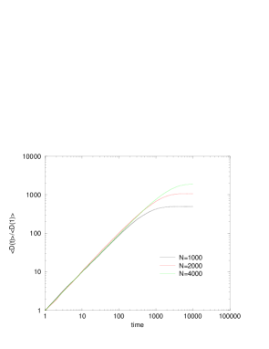
FIG. 1.: Distance $D(t)$ between the two replicas for three different sizes $N$ for the uncorrelated ring model.

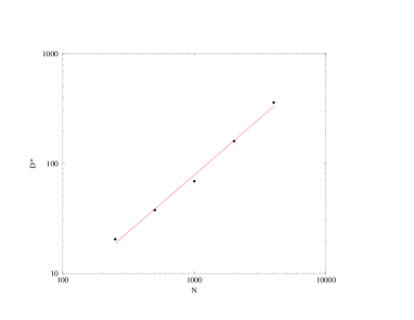
FIG. 2.: Scaling of the long time plateau $D^{*}=\frac{\langle D(\infty)\rangle}{\langle D(1)\rangle}$ as a function of the number of sites $N$ for the BS model. The best fit yields an exponent of $1.03(4)$.

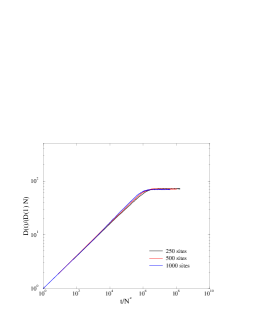
FIG. 3.: Collapse plot of the data for the evolution of the distance, in the BS case. The best fit yields $\alpha=0.32(3)$ and $z=3.0(2)$.

FIG. 4.: Extrapolation of $\alpha$ for the BS model with random updating.

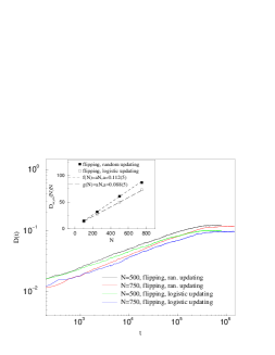
FIG. 5.: $\log_{10}$-$\log_{10}$ plot of $D(t)$ for the BS model with flipping, with random updating and deterministic updating with logistic map, for different system sizes. The value of the plateau actually depends on the updating rule, but it does not depend on the system size. Inset: A plot of the plateau of $ND(t)$ versus $N$ fits very well with a linear scaling, showing that the plateau of the Hamming distance $D(t)$ is size independent.

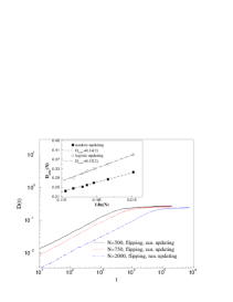
FIG. 6.: The $log_{10}-log_{10}$ plot of the Hamming distance $D(t)$ in the parallel BS model, versus the time $t$. Inset: logarithmic extrapolation of the plateau as a function of $N$, for both random and logistic updating rules. The infinite size value $D_{asym}$ obtained is in agreement with our analytical estimate.

FIG. 7.: Scaling of the effective DP-like time $t_{DP}$ with the Monte-Carlo time $t$, on a $log_{10}-log_{10}$ scale. We get a power law behavior with exponent $\zeta=1.41(2)$.

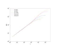
FIG. 8.: $log_{10}-log_{10}$ plot of the number $\sigma(t)$ of sites covered during the evolution of a single copy of the system, versus the time $t$, for random updating rule.

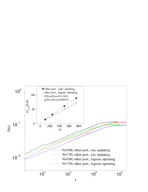
FIG. 9.: $\log_{10}$-$\log_{10}$ plot of $D(t)$ for the BS model with the perturbation (30), implementation (d), with random updating and deterministic updating with logistic map, for different system sizes. The value of the plateau actually depends on the updating rule, as in the flipping case. Inset: A plot of the plateau of $ND(t)$ versus $N$ gives the same findings of the case of flipping.

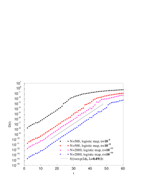
FIG. 10.: $linear$-$\log_{10}$ plot of $D(t)$ for the BS model with perturbation (30), implementation (d), and updating with a logistic map with parameter $b=4$, for different system sizes and mean initial distances $\epsilon$.

REFERENCES

- [1] J.M. Carlson and J.S. Langer, Phys. Rev. Lett. 62, 2632 (1989).
- [2] L. Gil and D. Sornette, Phys. Rev. Lett. 76, 3991 (1996).
- [3] P. Bak and K. Sneppen, Phys. Rev. Lett. 71, 4083 (1993).
- [4] R.V. Solé and J. Bascompte, Proc. R. Soc. Lond. B 263, 161 (1996); R.V. Solé and S.C. Manrubia, Phys. Rev. E 54, R42 (1996); R.V. Solé, J. Bascompte, and S.C. Manrubia, Proc. R. Soc. Lond. B 263, 1407 (1996).
- [5] M.Marsili, and A.Valleriani, Eur. Phys. J. B3, 417 (1998).
- [6] L.A. Nunes Amaral, and M. Meyer, Phys. Rev. Lett. 82, 652 (1999).
- [7] B. Drossel, Phys. Rev. Lett. 81, 5011 (1998).
- [8] K. Sneppen, Phys. Rev. Lett. 69, 3539 (1992); K. Sneppen, Phys. Rev. Lett. 71, 101 (1993).
- [9] D. Wilkinson and J.F. Willemsen, J. Phys. A 16, 3365; M. Cieplak and M.O. Robbins, Phys. Rev. Lett. 60, 2042 (1988).
- [10] P. Bak, C. Tang and K. Wiesenfeld, Phys. Rev. Lett. 59, 381 (1987).
- [11] D. Sornette, A. Johansen and I. Dornic, J. Physique I 5, 325 (1995).
- [12] C. Tsallis, A.R. Plastino and W.M. Zheng, Chaos, Solitons and Fractals 8, 885 (1997); U.M.S. Costa, M.L. Lyra, A.R. Plastino, and C. Tsallis, Phys. Rev. E. 56, 245 (1997); M.L. Lyra and C. Tsallis, Phys. Rev. Lett. 80, 53 (1998), A. R. R. Papa and C. Tsallis, Phys. Rev. E 57, 3923 (1998).
- [13] In [12], the behavior described by Eq. (2) has been related to the non-extensivity of the entropy proposed in C. Tsallis, J. Stat. Phys. 52, 479 (1988). Indeed, the exponent can be shown to be where is the extensivity parameter ( corresponding to the extensive case). We will not discuss this point further in this paper.
- [14] F.A. Tamarit, S.A. Cannas, and C. Tsallis, Eur. Phys. J. B 1, 545 (1998).
- [15] A. Valleriani and J.L. Vega, J. Phys. A 32, 105 (1999).
- [16] R. Cafiero, A. Valleriani, J.L. Vega, Eur. Phys. J. B 4, 405 (1998).
- [17] R. Cafiero, A. Valleriani, J.L. Vega, Eur. Phys. J. B 7, 505 (1999).
- [18] P. De Los Rios, A. Valleriani, and J.L. Vega, Phys. Rev. E 56 4876 (1997).
- [19] P. De Los Rios, A. Valleriani and J.L. Vega, Phys. Rev. E 57, 6451 (1998).
- [20] D. Sornette and I. Dornic, Phys. Rev. E 54, 3334 (1996).
- [21] H. E. Stanley, D. Stauffer, J. Kertész, and H. J. Hermann, Phys. Rev. Lett. 59, 2326 (1987); B. Derrida, Phys. Rep. 188, 207 (1989).
- [22] M. Paczuski, S. Maslov and P. Bak, Phys. Rev. E 53, 414 (1996).
- [23] P. Grassberger, Phys. Lett. A 200, 277 (1995).
- [24] Since, for finite every distribution has a cut-off, and therefore every moment is finite, this line of reasoning applies only in the limit . A more detailed analysis of this point has been presented elsewhere [16].
- [25] P. De Los Rios, M. Marsili, and M. Vendruscolo On the High-dimensional Bak-Sneppen model, cond-mat/9802069
- [26] H. Flyvbjerg, K. Sneppen, and P. Bak, Phys. Rev. Lett. 71, 4087 (1993)
- [27] H. Hinrichsen, J.S. Weitz, and E. Domany, J. Stat. Phys. 88, 617 (1997); P. Grassberger, J. Stat. Phys. 79, 13 (1995).
- [28] It is interesting to note that in the PBS the effect of the map is much smoother than in the case of the extremal BS [19]. This difference is certainly due to the fact that the effect of time correlation is “washed” out easier if the number of updated sites is big.