The validity of the Landau-Zener model for output coupling of Bose condensates

Abstract

We investigate the validity of the Landau-Zener model in describing the output coupling of Bose condensates from magnetic traps by a chirped radiofrequency field. The predictions of the model are compared with the numerical solutions of the Gross-Pitaevskii equation. We find a dependence on the chirp direction, and also quantify the role of gravitation.

Bose-Einstein condensation of alkali atoms in magnetic traps was first observed in 1995 [1]. The first step towards coherent matter beams was taken when a controlled release of condensed atoms from a magnetic trap was demonstrated in MIT [2], and recently at Garching [3]. The basic tool for output coupling has been spin-flipping induced by a radiofrequency (rf) magnetic field [2, 3], but other approaches have also been used [4, 5].

The MIT group demonstrated output couplings based on chirping the rf field, and on resonant rf pulses [2]. In both cases the experimental results are understood in terms of simple models. The theory of the pulsed and cw output couplings has been studied extensively in the literature [6, 7, 8, 9, 10]. In this Brief Report we examine the chirped output coupler. We find the validity conditions for the multistate Landau-Zener (MLZ) description [11] and compare them with the numerical solutions of the Gross-Pitaevskii (GP) equation [12]. We chart the combinations of the chirp speed $\lambda=d\omega_{\rm rf}/dt$ and the rf field amplitude $\Omega$ for which the MLZ description fails. We show that this failure depends on the chirp direction. Also, the repulsion between particles in the condensate and gravitation are found to contribute to the validity conditions.

Magnetic trapping is achieved by spin-polarising the atoms. For simplicity we consider the case of $F=1$, where $F$ is the hyperfine quantum number. In the inhomogeneous magnetic field the three substates $M=-1,0,1$ experience the potentials shown in Fig. 1(a). The atoms on the $M=-1$ state are trapped in the harmonic potential. In the MIT trap one had $\omega_{x}=\omega_{z}=(2\pi)\ 320$ Hz and $\omega_{y}=(2\pi)\ 18$ Hz [13]. When the spin of an atom is flipped from this state to the $M=0$ state, the atom moves away due to quantum mechanical dispersion and the repulsion between the condensed atoms. If the internal state of the atom is changed into the $M=1$ state, it feels the inverted parabolic potential as well.

FIG. 1.: Position dependence of the energy levels of atoms in a magnetic trap. (a) No output coupler, (b) output coupler with $\omega_{0}>\omega_{\rm rf}$, (c) output coupler with $\omega_{0}<\omega_{\rm rf}$.

We can eliminate the rf oscillations by making the rotating wave approximation, and then shifting each $M$ state in energy by an appropriate number of photons [14]. Now the field-induced resonances appear as potential crossings. At the rf field frequency $\omega_{0}$ the atoms at the center of the trap are in resonance with the field. We define the field detuning as $\Delta=\omega_{\rm rf}-\omega_{0}$. For $\Delta<0$ none of the atoms are in resonance, and for $\Delta>0$ atoms at locations $x=\pm x^{\prime}$ are in resonance [Fig. 1(b) and (c)].

In the chirped output coupler one sweeps $\omega_{\rm rf}$ so that all atoms in the trap feel a resonant field for a brief moment. The idea is to make this moment long enough for achieving a total or partial spin flip, and brief enough that the atoms do not have time to move due to changes in their internal state. Then the atoms remain stationary while they experience a time-dependent change of the energy difference between adjacent spin states.

In the MIT experiment a linear chirp was used: $\Delta=\lambda t$. For two internal states this corresponds directly to the Landau-Zener (LZ) model. In moderate magnetic fields the Zeeman shifts are linear and thus all adjacent states are resonant simultaneously, so one has a genuine multistate problem [11, 14]. In this particular case, however, the spin dynamics of a stationary atom can be described analytically, by a simple multistate generalization of the Landau-Zener result (MLZ) [11]. In the experiment the agreement with the MLZ prediction was good.

For simplicity we consider one spatial direction only. The three-state Hamiltonian for a stationary atom located at $x$ is

$$H(x,t)=\left(\begin{array}[]{ccc}\frac{1}{2}m\omega^{2}x^{2}-\hbar\Delta&\frac{\hbar\Omega}{\sqrt{2}}&0\\ \frac{\hbar\Omega}{\sqrt{2}}&0&\frac{\hbar\Omega}{\sqrt{2}}\\ 0&\frac{\hbar\Omega}{\sqrt{2}}&\hbar\Delta-\frac{1}{2}m\omega^{2}x^{2}\end{array}\right).$$ (1)

Here $m$ is the atomic mass, $\omega$ is the trap frequency and $\hbar\Omega$ is the rf field coupling. For a stationary atom we can solve the time-dependent Schrödinger equation with $H$. The MLZ theory predicts the final populations of the spin states:

$$P_{-1} = \exp(-2\pi\Gamma),$$ (2)

$$P_{0} = 2\exp(-2\pi\Gamma)[1-\exp(-2\pi\Gamma)],$$ (3)

$$P_{+1} = [1-\exp(-2\pi\Gamma)]^{2},$$ (4)

where $\Gamma=\Omega^{2}/(2\lambda)$ [2, 11]. In the MIT experiment $\lambda=(2\pi)\ 500$ MHz/s, and $\Omega$ changed from 0 to about $(2\pi)\ 11.3$ kHz. The $P_{i}$’s depend only on $\Gamma$ and not on the trap geometry; thus in asymmetric traps the output coupling takes place in all directions with the same efficiency.

In the Gross-Pitaevskii theory the single atom amplitudes $\Psi_{i}(x,t)$ describe effectively the whole condensate (i.e., $|\Psi_{i}(x,t)|^{2}$ gives the density distribution of the atoms on spin state $i$) [12]. Their time evolution is obtained from the time-dependent Schrödinger equation with the Hamiltonian

$${\cal H}_{i,j}=-\frac{\hbar^{2}}{2m}\frac{\partial^{2}}{\partial x^{2}}\delta_{i,j}+H_{i,j}+\sum_{l=1}^{3}C_{i,l}|\Psi_{l}|^{2}.$$ (5)

The last term describes interactions between the particles. The parameters $C_{i,l}$ are proportional to atom numbers and the scattering lengths of the corresponding internal states $i$ and $l$. In our one-dimensional study this parameter does not match properly with the realistic three dimensional situation. But a trap with a very low frequency at one direction can be regarded quasi one-dimensional. In this case a reasonable estimate for our 1D $C$ parameter would be $C=C_{3D}/A$, where $A$ is the cross sectional condensate area. As an order of magnitude estimate it should be valid for other traps as well. For simplicity we take all $C$’s to be equal.

We solve the GP equation numerically for the output coupler. In the limit of large $C$ we can ignore the kinetic energy term and obtain the Thomas-Fermi solution, $\Psi(x,0)=\sqrt{[\mu-U(x)]/C}$, where $U(x)$ is the trapping potential. The condition $\mu-U(x)\geq 0$ defines the edge of the condensate. The chemical potential $\mu$ is obtained from the normalisation of the wave function.

A breakdown of the MLZ model is expected if the atoms move during the transition process. A similar problem arises for diatomic molecules interacting with short laser pulses [15]. In order to quantify this breakdown we consider the characteristic time scale $\delta t$ of the LZ process, $\delta t\simeq\Omega/\lambda$ [16]. The atoms need to remain stationary during this time. The term ”stationary” can be defined by transforming $\delta t$ into a region $\delta x$ around the location $x_{0}$ of the atom. For simplicity we assume that $x_{0}>0$. For parabolic potentials in the $F=1$ case we set $\hbar\Omega=\frac{1}{2}m\omega^{2}[(x_{0}+\delta x)^{2}-x_{0}^{2}]\simeq m\omega^{2}x_{0}\delta x$, which defines $\delta x$. If the atom moves a distance $\Delta x$ in time $\delta t$, it can be regarded stationary if $\Delta x\ll\delta x$.

The atomic motion can arise from quantum mechanical diffusion, repulsion between atoms, or from acceleration along the inverted parabolic potential. We consider the acceleration $a$ first. With Newtonian dynamics we get $a(x_{0})=-(1/m)(\partial U/\partial x)|_{x=x_{0}}=\omega^{2}x_{0}$. In the small region around $x_{0}$ we have $\Delta x=a(\delta t)^{2}/2=\omega^{2}x_{0}\Omega^{2}/(2\lambda^{2})$. Thus we get the condition $\lambda^{2}/\Omega\gg m\omega^{4}x_{0}^{2}/\hbar$. This needs to be true for all $x_{0}$; the right-hand side is maximised at the edge of the condensate.

For small $C$ the edge is near the width of the ground state of the harmonic potential, max$(x_{0})\simeq\sqrt{\hbar/m\omega}$, which gives

$$\frac{\lambda^{2}}{\Omega\omega^{3}}\gg 1.$$ (6)

For large $C$ we take the Thomas-Fermi approximation, and then max$(x_{0})\simeq\sqrt{2\mu/m\omega^{2}}$, which gives

$$\frac{\lambda^{2}}{\Omega\omega^{2}}\gg\omega_{\mu},$$ (7)

where $\mu=\hbar\omega_{\mu}$. The MIT trap parameters satisfy condition (6) well in all directions, and to break down condition (7) would require an unrealistically large $\mu$. Since $\lim_{C\rightarrow 0}\mu=\hbar\omega/2$, Eq. (6) is a special case of Eq. (7).

Diffusion and repulsion can give atoms a velocity which initially overcomes the acceleration. For the $M=0$ state these processes are naturally covered by the various studies of the ballistic expansion of condensates; see Ref. [17] and references therein. As we are only looking for constraints it is sufficient to characterise the maximum speed $v$ of the atoms with the energy stored in the trapped condensate. We set $\mu=mv^{2}/2$. For small $C$ the speed $v$ reduces to the free-space momentum width of the Gaussian harmonic oscillator wave function, $v\simeq\sqrt{\hbar\omega/m}$. Now $\Delta x\simeq v\delta t$. On the other hand, at $x_{0}=0$ we have $\delta x=\sqrt{2\hbar\Omega/(m\omega^{2})}$. Eventually we get for diffusion/repulsion the conditions (6) and (7).

These conditions do not depend on the direction of the chirp. However, there exists another breakdown mechanism for the MLZ theory. Atoms that have interacted resonantly with the field can re-enter the resonance region (a reunion) due to their motion. Let us consider a positive chirp: a resonance emerges at $x=0$ and then separates into two points that move towards large $|x|$. This is demonstrated in Fig. 1 if we consider it as a sequency of snapshots. Strong acceleration on the $M=1$ state leads to the above problem. We need a condition on $\lambda$ and $\Omega$ for avoiding the reunion until the transition probability is negligible.

Here the direction of the chirp is crucial. For negative chirps the resonances emerge at large $|x|$ and move towards $x=0$ where they disappear. Acceleration, however, moves the atoms in the opposite direction. Thus for negative chirps the reunion problem is absent. The role of chirp direction has been studied e.g. in the context of laser-molecule interactions [15].

We consider the case where the reunion happens at $x=x_{0}$. Energy conservation gives us roughly the local speed $v_{0}$ of the moving atoms: $v_{0}\simeq\omega x_{0}$. The slope of the local energy difference between adjacent states is $\alpha_{0}=m\omega^{2}x_{0}$. The product of these quantities gives us the local motion-induced change in the energy levels for the atom: $\hbar\lambda_{0}=|dU/dt|=|(\partial U/\partial x)(\partial x/\partial t)|_{x=x_{0}}=m\omega^{3}x_{0}^{2}$. The motion of the resonance, $\lambda$, is small compared to $\lambda_{0}$ for realistic parameters, and we can ignore it. Basically, we want that the motion-induced LZ transition probability at $x_{0}$ is smaller than some fixed value $\tilde{\Gamma}$:

$$\Gamma=\frac{\Omega^{2}}{\lambda_{0}}\leq\tilde{\Gamma}.$$ (8)

The time it takes for a resonance to reach $x_{0}$ is $t_{0}=m\omega^{2}x_{0}^{2}/(2\hbar\lambda)$. For a accelerating atoms we need to solve the Newtonian equation of motion: $(\partial^{2}x/\partial t^{2})-\omega^{2}x=0$. For $x^{\prime}=\sqrt{2\hbar\lambda t^{\prime}/(m\omega^{2})}$, $v(t^{\prime})=v^{\prime}$ we get

$$x=x^{\prime}\cosh[\omega(t-t^{\prime})]+\frac{v^{\prime}}{\omega}\sinh[\omega(t-t^{\prime})].$$ (9)

There are several possible values for $x^{\prime}$ and $v^{\prime}$, and the quantum mechanical diffusion/repulsion complicates this simple Newtonian picture. For large $C$ we can assume that the particles which reach the reunion first come from the edge of the initial condensate. This fixes $x^{\prime}$ (and $t^{\prime}$). We have simulated the problem numerically with the GP equation, and obtained the reunion time for the fastest atoms. As shown in Fig. 2(a) an effective trajectory $v^{\prime}\propto C^{1/3}$ locates the reunion well. The main dependence on $C$, however, arises from the location of the condensate edge, $x^{\prime}\propto C^{1/3}$. Some examples of the breakdown are shown in Fig. 2(b).

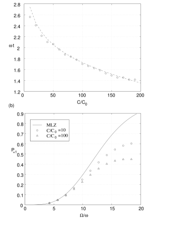
FIG. 2.: (a) The time it takes for the spin-flipped atoms to reach the reunion as a function of $C$, and when and $\lambda=100\omega^{2}$. The circles are the GP results, and the dashed line is the classical estimate based on Eq. (9). (b) The breakdown of the MLZ theory as a function of $\Omega$ for two values of $C$, and $\lambda=200\omega^{2}$. Here $C_{0}=\sqrt{\hbar^{3}\omega/m}$.

One should not make detailed conclusions from such trajectories. Apart from the crudeness of the Newtonian mechanics, the fastest atoms are only a fraction of the condensate. In Fig. 3 we show in the ($\lambda,\Omega$) plane where the MLZ prediction for $P_{+1}$ fails for more than 10 % for the large $C$ case. The constraint obtained by using the effective trajectory and condition (8) is clearly too demanding. Also, in a real experiment one can switch the field off before the reunion and thus avoid the problem. This is the case in the MIT experiment: after reaching the resonance $\omega_{0}$ the rf field is on for about $\tau\simeq 0.5$ ms. As $\tau\omega_{x}=1$ and $\tau\omega_{y}=0.06$, the field is off by the time of reunion, as Fig. 2(a) shows. For a negative $\lambda$ we saw no large deviation from the MLZ prediction for the values used in Fig. 3.

The effects of gravitation should be considered in output couplers [9, 18]. In the direction of gravitation ($z$) the trapping potentials are

$$V_{-1} = \frac{1}{2}m\omega_{z}^{2}\left(z+\frac{g}{\omega_{z}^{2}}\right)^{2}-\frac{mg^{2}}{2\omega_{z}^{2}},$$ (10)

$$V_{0} = mgz$$ (11)

$$V_{+1} = -\frac{1}{2}m\omega_{z}^{2}\left(z-\frac{g}{\omega_{z}^{2}}\right)^{2}+\frac{mg^{2}}{2\omega_{z}^{2}},$$ (12)

where $g$ is the gravitational acceleration. The $M=\pm 1$ potentials remain harmonic but have spatially shifted centers, as shown in Fig. 4. As gravitation affects only the external degrees of freedom the rf field resonance conditions still follow the purely magnetic potentials. In other words, the resonance points are located symmetrically in respect to the magnetic field minimum, but not in respect to the trap center. For a stationary atom the LZ parameter $\Gamma$ remains unaffected by gravitation, but many other conditions change.

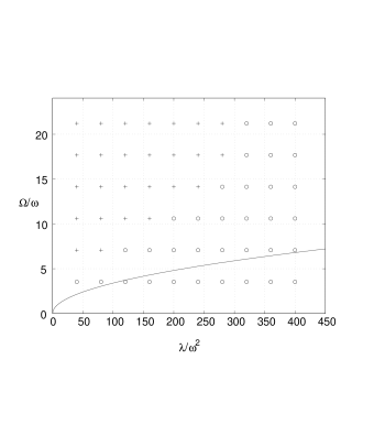
FIG. 3.: The validity of the MLZ theory. The model predictions for $P_{+1}$ are compared with the GP solutions for the case of positive ($\lambda>0$) chirp direction. Here $C=100C_{0}$, which corresponds well to the Thomas-Fermi limit. The plus signs ($+$) indicate when the values differ by more than 10 %, and circles when less. In the region below the solid line the reunion is not expected to produce more than 10 % deviation even if all atoms on the $M=+1$ state would reach the reunion as soon as the first ones do it in simulations.

For the MIT trap one gets $(\Delta x)_{g}=g/\omega_{z}^{2}=2.5\ \mu$m which is about the size of the trap ground state (1.7 $\mu$m) but clearly smaller than the condensate (17 $\mu$m). For gravitation to dominate acceleration on the $M=1$ state at the condensate edge we obtain the condition $2\mu\omega_{z}^{2}<mg^{2}$ (for large $C$), which reduces to $\hbar\omega_{z}^{2}<mg^{2}$ as $C\rightarrow 0$. If gravitation dominates, then the basic validity condition for the MLZ approach becomes ($\Delta z=g\Omega^{2}/\lambda^{2}$, $\delta z=\hbar\Omega/(m\omega_{z}^{2}z_{0})$, $z_{0}\simeq g/\omega_{z}^{2}$)

$$\frac{\lambda^{2}}{\Omega}\gg\frac{mg^{2}}{\hbar}.$$ (13)

This applies also for the motion on the $M=0$ state.

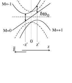
FIG. 4.: Position dependence of the energy levels of atoms in a magnetic trap under the effect of gravitation. The shift factor for the potential centers is $z^{\prime}=g/\omega^{2}$. The dashed lines show the magnetic trap potentials without the effect of gravitation $\vec{g}$.

Figure 4 shows also that the shifts in the potential centers can be used for directed output coupling. With a very slow negative chirp one can leak the condensate from the earthside edge of the trap, as the chirped rf pulse becomes resonant there first. Due to the slowness the condensate edge will follow the resonance, and the other resonance point will not reach the diminishing condensate. This approach is used in the recent experiment [3]. It is complementary to the situation considered by us, as there the chirp timescale must be clearly longer than the motional time scales.

In this Brief Report we have derived the validity conditions of the multistate Landau-Zener approach for chirped output couplers, with and without the presence of gravitation. Comparison with numerical results shows that these conditions allow one to achive ”safe” parameter regions easily in the experiments. Our study is for one dimension only, but our results should apply directly to three dimensions, especially in the case of strongly asymmetric traps, where the tightest trapping direction will dominate the expansion of the untrapped atom cloud.

We acknowledge the support by the Academy of Finland.

REFERENCES

- [1] M. H. Anderson, J. R. Ensher, M. R. Matthews, C. E. Wieman, and E. A. Cornell, Science 269, 198 (1995); K. B. Davis, M.-O. Mewes, M. R. Andrews, N. J. van Druten, D. S. Durfee, D. M. Kurn, and W. Ketterle, Phys. Rev. Lett. 75, 3969 (1995).
- [2] M.-O. Mewes, M. R. Andrews, D. M. Kurn, D. S. Durfee, C. G. Townsend, and W. Ketterle, Phys. Rev. Lett. 78, 582 (1997).
- [3] I. Bloch, T. W. Hänsch, and T. Esslinger, Phys. Rev. Lett. 82, 3008 (1999).
- [4] B. P. Anderson and M. A. Kasevich, Science 282, 1686 (1998).
- [5] E. W. Hagley, L. Deng, M. Kozuma, J. Wen, K. Helmerson, S. L. Rolston, and W. D. Phillips, Science 283, 1706 (1999).
- [6] R. J. Ballagh, K. Burnett, and T. F. Scott, Phys. Rev. Lett. 78, 1607 (1997).
- [7] M. Naraschewski, A. Schenzle, and H. Wallis, Phys. Rev. A 56, 603 (1997); H. Steck, M. Naraschewski, and H. Wallis, Phys. Rev. Lett. 80, 1 (1998).
- [8] B. Jackson, J. F. McCann, and C. S. Adams, J. Phys. B 31, 4489 (1998).
- [9] R. Graham and D. F. Walls, Phys. Rev. A 60, 1429 (1999).
- [10] Y. B. Band, P. S. Julienne, and M. Trippenbach, Phys. Rev. A 59, 3823 (1999).
- [11] N. V. Vitanov and K.-A. Suominen, Phys. Rev. A 56, R4377 (1997).
- [12] P. Nozieres and D. Pines, The Theory of Quantum Liquids, Vol II (Redmond City, Addison-Wesley, 1990).
- [13] K. B. Davis, M.-O. Mewes, M. R. Andrews, N. J. van Druten, D. M. Kurn, D. S. Durfee, and W. Ketterle, Phys. Rev. Lett. 77, 416 (1996).
- [14] W. Ketterle and N. J. van Druten, Adv. At. Mol. Opt. Phys. 37, 181 (1996).
- [15] B. M. Garraway and K.-A. Suominen, Rep. Prog. Phys. 58, 365 (1995); A. Paloviita, K.-A. Suominen, and S. Stenholm, J. Phys. B 28, 1463 (1995).
- [16] N. V. Vitanov, Phys. Rev. A 59, 988 (1999).
- [17] A. S. Parkins and D. F. Walls, Phys. Rep. 303, 1 (1998).
- [18] M. W. Jack, M. Naraschewski, M. J. Collett, and D. F. Walls, Phys. Rev. A 59, 2962 (1999).