[

Magnetoresistance of magnetic multilayers in the CPP mode:
evidence for non-local scattering

Abstract

We have carried out measurements of the magnetoresistance MR(H) in the CPP (Current Perpendicular to the Plane) mode for two types of magnetic multilayers which have different layer ordering. The series resistor model predicts that CPP MR(H) is independent of the ordering of the layers. Nevertheless, the measured MR(H) curves were found to be completely different for the following two configurations: [Co(10Å)/Cu(200Å)/Co(60Å)/Cu(200Å)]_N and [Co(10Å)/Cu(200Å)]_N [Co(60Å)/Cu(200Å)]_N showing that the above model is incorrect. We have carried out a calculation showing that these results can be explained quantitatively in terms of the non-local character of the electron scattering, without the need to invoke spin-flip scattering or a short spin diffusion length.

]

Since the discovery a decade ago of the giant magnetoresistance exhibited by magnetic multilayers, interest in this phenomenon has not abated [1]. Recent research has focused on the magnetoresistance MR(H) in the CPP mode (current perpendicular to the plane of the layers) [2, 3, 4, 5, 6]. Measurements of MR(H) are technically more difficult in the CPP mode than in the CIP mode (current in plane). However, there are advantages to the MR(H) data in the CPP mode. For example, it has been shown [7, 8] that experimental values of MR(H) in the CPP mode can shed light on the spin diffusion length. Here we present evidence for the importance of MR(H) measurements in the CPP mode for determining the role of non-local electron scattering in the giant magnetoresistance (GMR). We shall show that because of the long electron mean free path, non-local scattering makes the series resistor model inappropriate.

As is well known, the GMR occurs in magnetic multilayers because the spin-up electrons and the spin-down electrons have different scattering rates. If the electron does not flip its spin upon scattering, then the spin-up and spin-down electrons constitute two separate currents, with different resistivities, as if flowing in two parallel wires. In the CPP mode, the resistances of the different layers add in series [1, 7, 8]. Therefore, it would seem that two magnetic multilayers that differ only in the ordering of the layers would yield identical results for MR(H) in the CPP mode.

To test this idea, Pratt and co-workers at Michigan State University (Chiang $et$ $al.$ [9]) measured CPP MR(H) for the two configurations [Py/Cu/Co/Cu]_N and [Py/Cu]_N[Co/Cu]_N (denoted as ‘interleaved’ and ‘separated’ configurations, respectively), where Py is Ni₈₄Fe₁₆. Although the expectation was that identical MR(H) curves would be obtained for the interleaved and the separated configurations, these workers found that the resulting two MR(H) curves were completely different. Chiang $et$ $al.$[9] attributed their results to the short spin diffusion length in Py. They had previously analyzed resistivity data within the framework of Valet-Fert theory [7, 8] and obtained [10] for Py a spin diffusion length of only 55 Å, thus implying significant mixing between the spin-up and spin-down electron currents. Chiang $et$ $al.$ proposed that this spin-flipping was responsible for the different CPP MR(H) curves they observed for the separated and interleaved configurations.

We have investigated these ideas by measuring MR(H) for multilayers whose magnetic layers do $not$ exhibit a short spin diffusion length. For the different magnetic layers, we used Co of two different thicknesses, since Co is known [11, 12] to have a long spin diffusion length. Measurements were carried out of CPP MR(H) for [Co(10Å)/Cu(200Å)/Co(60Å)/Cu(200Å)]_N and [Co(10Å)/Cu(200Å)]_N[Co(60Å)/Cu(200Å)]_N for
N = 4, 6, 8. The thickness (200 Å) of the non-magnetic layers was chosen to be large enough to ensure complete magnetic decoupling between the ferromagnetic layers. In spite of the fact that the interleaved and separated configurations differ only in the ordering of the layers, the measured MR(H) curves were found to be very different for the two different configurations. We shall show that these results can be explained quantitatively in terms of non-local electron scattering.

The multilayers were grown in our VG-80M MBE facility which has base pressure of typically 4$\times 10^{-11}$ mbar. Our CPP measurements used the superconducting Nb electrode technique, as developed by Pratt et al. [2]. The superconducting equipotential [3, 4] ensures that the current is perpendicular to the layers. We used a SQUID-based current comparator, working at 0.1${\%}$ precision to measure changes in the sample resistance of order 10 p$\Omega$. To avoid driving the Nb normal, the CPP measurements were performed at 4.2 K in magnetic fields below 3 kOe. Consistency between the interleaved and separated samples was enhanced by growing the two configurations during the same run for each value of N.

The magnetoresistance was measured in the CPP mode for the two configurations: interleaved and separated. The measured curves for MR(H) are presented for three values of N in Figs. 1a-1c. The squares represent the MR(H) data in the interleaved configuration whereas the circles give the data in the separated configuration. For each sample, the saturation magnetic field was about 2 kOe.

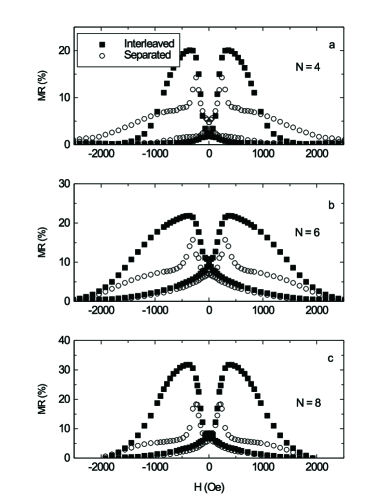
FIG. 1.: Magnetic field dependence of the magnetoresistance MR(H) for the interleaved (squares) and separated (circles) multilayers containing Co (10Å) and Co (60Å) as the two magnetic metals, for the indicated number of repeats.

There are several characteristic features of these data, all of which can be explained in terms of non-local electron scattering. (i) The most important feature is surely the striking difference between the MR(H) curves for the two configurations, both in shape and in magnitude.
(ii) For each N, the maximum value of MR(H) is larger for the interleaved configuration. (iii) The MR(H) curve for the interleaved configuration exhibits a single peak, whereas for the separated configuration, MR(H) is the superposition of two peaks, with the second being much broader and less delineated than the first. Another interesting feature of the data, not displayed in Fig. 1, is that the saturated resistance itself is always greater for the interleaved configuration.

To ensure that the differing results for MR(H) for the two configurations are not due to differences in their magnetic properties, the magnetization as a function of field was measured for each sample. We found that the two configurations yield the same magnetization. This confirms that the magnetic layers are uncoupled and become magnetized independently. At low fields, the magnetization curves are dominated by the contribution of the thicker Co layers. After the thicker Co layers reach saturation, the magnetization continues to increase as the thinner Co layers approach saturation. The magnitudes of the saturation fields for the two thicknesses of Co layers correspond closely to the saturation fields of MR(H).

Kinetic theory arguments show that the electron mean free path is far longer than the thicknesses of the magnetic layers (10 Å and 60 Å). Therefore, the potential ”felt” by the electron is the combined potential of a neighboring pair of magnetic layers. This may be termed ”non-local” electron scattering in the sense that one cannot speak of the resistivity of a $single$ Co layer. Rather, the resistivity is determined by a property of $pairs$ of neighboring layers. Gittleman $et$ $al.$ [13] have shown that for such a case, the contribution of the spin-direction-dependent resistivity depends on the cosine of the angle $\theta_{ij}$ between the moments of neighboring magnetic layers, i and j. This is the key to understanding the data.

Because the mean free path is larger than the layer thicknesses, it is necessary to carry out a full band structure calculation to calculate properly the resistivity and magnetoresistance. However, one can understand the basic physics with a simple phenomenological model.

For the interleaved configuration, the neighboring magnetic layers are different, and hence the maximum angle $\theta_{ij}$ is large, whereas for the separated configuration, the neighboring magnetic layers are the same (except for one boundary layer), and hence the maximum angle $\theta_{ij}$ is small. Therefore, there is no reason to expect MR(H) to be the same for the two configurations. This explains the first feature of the data mentioned above.

From the above considerations, it also immediately follows that MR(H) will be larger for interleaved multilayers than for separated multilayers, because the angle $\theta_{ij}$ is larger for the former configuration. This explains the second feature of the data mentioned above. This has been confirmed by measurements of the GMR as a function of the number of bilayers. A Fuchs-Sondheimer analysis of these data shows that the mean free path in sputtered [14] and MBE [15] samples is about 500 Å and 700 Å, respectively.

For the interleaved configuration, there is only $one$ angle $\theta_{ij}$ that is relevant, namely, the angle between the moments of the different (10Å and 60Å) neighboring magnetic layers. Therefore, there will be only $one$ peak, as the angle $\theta_{ij}$ becomes progressively larger, passes through a maximum at the saturation field of the Co (60Å) layer and then becomes smaller as the Co (10Å) layer also saturates. By contrast, for the separated configuration, there are $two$ angles $\theta_{ij}$ that are relevant, namely, the angle between neighboring moments for each set of layers (the 10 Å set and the 60 Å set). As each angle $\theta_{ij}$ passes through its maximum, a peak will be obtained for MR(H), leading to two overlapping peaks, with each maximum occurring at a different value of the magnetic field, corresponding roughly to the coercive field of each type of magnetic layer. This explains the third feature of the data mentioned above.

These ideas can be made quantitative. If the spin diffusion length is very long, it is known [1] that a simple expression is obtained for MR(H). According to the phenomenological theory of Wiser [17], for the geometry under consideration here and assuming a very long spin diffusion length, the magnetoresistance due to an $ij$-pair of neighboring magnetic layers is:

$$MR_{ij}(H)=c_{ij}(1-\cos\theta_{ij}(H))^{2}$$ (1)

The spin diffusion length of Co has been measured yielding values of 450 Å [11, 12] and 1000 Å [9]. These values is very much larger than the thickness of the Co layers, and so one may safely employ the expression for MR(H) given in (1).

For our samples, there are three parameters $c_{ij}$ corresponding to the three different types of neighboring pairs of magnetic layers: i = j = 1; i = j = 2; i = 1, j = 2, where 1 refers to Co (60Å) layers and 2 refers to Co (10Å) layers. The interleaved configuration contains only type i = 1, j = 2 neighbors, whereas the separated configuration contains all three types. For a sample containing N repeats, the separated configuration consists of N-1 pairs of type i = j = 1 neighbors, followed by one pair of type i = 1, j = 2 neighbors (the boundary layer), followed by N-1 pairs of type i = j = 2 neighbors.

First consider the interleaved configuration. The saturation magnetic field $H_{s1}$ of the thicker Co layers is smaller than $H_{s2}$ of the thinner Co layers. Thus, as the magnetic field is increased, the angle $\theta_{1,2}$ increases, since the thicker Co layers are reversing their direction of magnetization faster than the thinner Co layers. According to Eq. (1), increasing the angle $\theta_{1,2}$ implies an increase in MR(H). When the magnetic field reaches $H_{s1}$, the angle $\theta_{1,2}$ reaches its maximum value, and begins to decrease as the thinner Co layers continue to reverse their direction of magnetization while the thicker Co layers have already reached saturation. According to Eq. (1), decreasing $\theta_{1,2}$ leads to a decrease in MR. Finally, when the field reaches $H_{s2}$, the angle $\theta_{1,2}$ is again zero, and MR vanishes. Thus, we expect - and find - a single peak for MR(H) for the interleaved configuration.

The field dependence of $\theta_{ij}$ is determined as follows. The magnetization increases linearly with field (except near saturation, where it increases more slowly). Since the magnetization is proportional to the cosine of the angle between the magnetic moment and the field, it follows that cos$\theta_{i}$ and cos$\theta_{j}$ are each linear in the field. Equation (1) contains cos$\theta_{ij}$ = cos($\theta_{i}$ - $\theta_{j}$). Expanding the cosine readily gives the required field dependence.

The calculated results [17] for the interleaved configuration are given by the curves in Fig. 2. For each value of N, the parameter $c_{1,2}$ was determined by fitting to the MR(H) data. The agreement between the calculated curves and the data is evident from the figure.

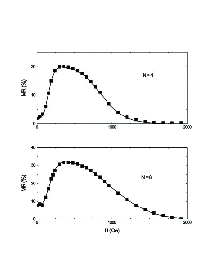
FIG. 2.: Comparison between the calculated curves (solid lines) and the data points (squares) for MR(H) for the interleaved configuration for the indicated number of repeats.

We now consider the separated configuration. If the Co layers were ideal single-domain structures, then the magnetic moment of each Co layer would react identically to the magnetic field and the angles $\theta_{1,1}$ and $\theta_{2,2}$ would both be zero at all fields. However, because of the presence of domains and of structural imperfections in the Co layers, each layer reverses its magnetization at a somewhat different rate. As a result, the angles $\theta_{1,1}$ and $\theta_{2,2}$ become non-zero as the field is increased, pass through a maximum at the coercive field, and then decrease to zero as saturation is approached.

We assumed a simple parabolic form for each of the two angles. The maximum value of each parabola, $\theta_{max,1,1}$ and $\theta_{max,2,2}$, cannot be determined by fitting to the data for the following reason. Because these angles are small, Eq. (1) can be expanded to yield

$$MR_{ii}=c_{ii}(\frac{1}{2}\theta_{ii}^{2})^{2}\propto c_{ii}(\theta_{max,ii})^{4}$$ (2)

and this $combination$ of $c_{ii}$ and $\theta_{max,ii}$ serves as a $single$ fitting parameter. Nevertheless, some numerical tests we have carried out suggest that both $\theta_{max,1,1}$ and $\theta_{max,2,2}$ lie in the range of $15^{\circ}-30^{\circ}$. This value is, of course, much smaller than the maximum value of the angle $\theta_{1,2}$. This explains why MR(H) is larger for the interleaved configuration than for the separated configuration.

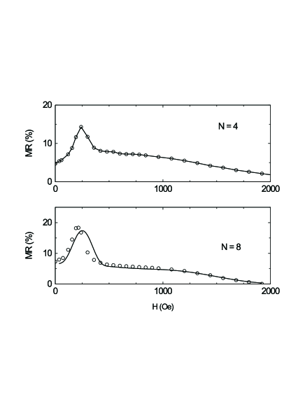
FIG. 3.: Comparison between the calculated curves (solid lines) and the data points (circles) for MR(H) for the separated configuration for the indicated number of repeats.

The calculated results [17] for the separated configuration are given by the curves in Fig. 3. For each value of N, the three parameters $c_{1,1}(\theta_{max,1,1})^{4}$, $c_{2,2}(\theta_{max,2,2})^{4}$, and $c_{1,2}$ were determined by fitting to the MR(H) data. The agreement between the calculated curves and the data is evident from the figure.

To confirm that MR(H) for the separated configuration contains the contributions of [Co(10Å)/Cu(200Å)]_N and of [Co(60Å)/Cu(200Å)]_N, we also measured MR(H) for a multilayer containing only [Co(10Å)/Cu(200Å)]_N and for another multilayer containing only [Co(60Å)/Cu(200Å)]_N. For each of these two multilayers, MR(H) consists of a single peak, located at the same magnetic field as one of the two peaks in the separated configuration. Thus, the two peaks observed for the separated configuration do indeed correspond to the two individual peaks.

In conclusion, we have shown that the principal features of the MR(H) data can be explained quantitatively, for both the interleaved and the separated configurations, by invoking non-local electron scattering.

It is a pleasant duty to acknowledge that this research was supported by grants from the UK-Israel Science and Technology Research Fund and the UK-EPSRC. We appreciate discussions with C. H. Marrows and A. Carrington. D. Bozec thanks the University of Leeds for financial support.

REFERENCES

- [1] M. N. Baibich, J. M. Broto, A. Fert, F. N. Vandau, F. Petroff, and P. Etienne, Phys. Rev. Lett. 61, 2472 (1988); S. S. P. Parkin, Phys. Rev. Lett. 71, 1641 (1993); R. E. Camley and J. Barnas, Phys. Rev. Lett. 63, 664 (1989); J. Mathon, Contemp. Phys. 32, 143 (1991); S. Y. Hsu, A. Barthelemy, P. Holody, R. Loloee, P. A. Schroeder, and A. Fert, Phys. Rev. Lett. 78, 2652 (1997); J. A. Borchers, J. A. Dura, J. Unguris, D. Tulchinsky, M. H. Kelley, C. F. Majkrzak, S. Y. Hsu, R. Loloee, W. P. Pratt, Jr., and J. Bass, Phys. Rev. Lett. 82, 2796 (1999).
- [2] W. P. Pratt, Jr., S.-F. Lee, J. M. Slaughter, R. Loloee, P. A. Schroeder, and J. Bass, Phys. Rev. Lett. 66, 3060 (1991).
- [3] N. J. List, W. P. Pratt, Jr., M. A. Howson, J. Xu, M. J. Walker, and D. Greig, J. Magn. Magn. Mater. 148, 342 (1995).
- [4] N. J. List, W. P. Pratt, Jr., M. A. Howson, J. Xu, M. J. Walker, B. J. Hickey, and D. Greig, Mat. Res. Soc. Symp. Proc. 384, 329 (1995).
- [5] S.-F. Lee, W. P. Pratt, Jr., Q. Yang, P. Holody, R. Loloee, P. A. Schroeder, and J. Bass, J. Magn. Magn. Mater. 118, L1 (1993).
- [6] S.-F. Lee, Q. Yang, P. Holody, J. H. Hetherington, S. Mahmood, B. Ikegami, K. Vigen, L. L. Henry, P. A. Schroeder, W. P. Pratt, Jr., and J. Bass, Phys. Rev. B 52, 15426 (1995).
- [7] T. Valet and A. Fert, Phys.Rev. B 48, 7099 (1993).
- [8] A. Fert and S.-F. Lee, Phys. Rev. B53, 6554 (1996).
- [9] W.-C. Chiang, Q. Yang, W. P. Pratt, Jr., R.Loloee, and J. Bass, J. Appl. Phys. 81, 4570 (1997).
- [10] S. D.Steenwyk, S. Y. Hsu, R. Loloee, J. Bass, and W. P. Pratt, Jr., J. Magn. Magn. Mater. 170, L1 (1997).
- [11] L. Piraux, S. Duboix, C. Marchal, J. M. Beuken, L. Filipozzi, J. F. Depres, K. Ounadjela, and A. Fert, J. Magn. Magn. Mater. 156, 317 (1996).
- [12] L. Piraux, S. Duboix, A. Fert, and L. Belliard, European Phys. J. 4, 413 (1998).
- [13] J. L. Gittleman, Y. Goldstein, and S. Bozowski, Phys. Rev. B 5, 3609 (1972).
- [14] T.S. Plaskett and T.R Macquire, J. Appl. Phys. 73, 6378 (1993); C. H. Marrows, PhD Thesis, University of Leeds, 1998.
- [15] K. Wellock, PhD Thesis, University of Leeds, 1996.
- [16] N. Wiser, J. Magn. Magn. Mater. 159, 119 (1996).
- [17] N. Wiser, to be published.