Scale-invariant Truncated Lévy Process

Abstract

We develop a scale-invariant truncated Lévy (STL) process to describe physical systems characterized by correlated stochastic variables. The STL process exhibits Lévy stability for the probability density, and hence shows scaling properties (as observed in empirical data); it has the advantage that all moments are finite (and so accounts for the empirical scaling of the moments). To test the potential utility of the STL process, we analyze financial data.

In recent years, the Lévy process [1] has been proposed to describe the statistical properties of a variety of complex phenomena [2, 3, 4, 5, 6, 7, 8, 9]. The Lévy process is characterized by “fat tails” (power law), and display scaling behavior similar to that observed in a wide range of empirical data. However, the application of the Lévy process to empirical data is limited because it is characterized by infinite second and higher moments, while empirical data have finite moments.

Truncated Lévy (TL) processes are defined to have a Lévy probability density function (PDF) in the central regime, truncated by a function decaying faster than a Lévy distribution in the tails [10]. The TL process is introduced to account for the finite moments observed for empirical data [11]. However, the TL process (with either abrupt [10] or smooth [12] truncation) has limitations when applied to empirical data. (i) The TL process is introduced for independent and identically distributed (i.i.d.) stochastic variables, while variables describing many physical systems are not i.i.d. — e.g. there are correlations. (ii) The PDF of the TL process tends to the Gaussian distribution (according to the central limit theorem), and hence does not exhibit scale invariance; PDFs for a variety of complex systems, however, are often characterized by regions of scale-invariant behavior. (iii) The time scale above which the Lévy profile becomes Gaussian depends on the size of the truncation cutoff (or the standard deviation) [10, 12]; to mimic the Lévy type scale invariant behavior observed for data, the TL process must be defined with a standard deviation larger than the one observed for the data [see caption to Fig.1].

Here we introduce a type of stochastic process which we call the scale-invariant truncated Lévy (STL) process. Stochastic variables $z$ in the STL are generated by the symmetrical probability function $f(z)=Ae^{-\lambda|z|^{\beta}}|z|^{-1-\alpha}$, where $0<\alpha<2$ [13]. The exponential prefactor [12] ensures a smooth truncation of the Lévy distribution, where the parameter $\beta$ can take any positive value [14], $\lambda^{-1}$ is related to the size of the truncation cutoff, and $A$ is a measure of the “spread” in the central region.

From the probability function $f(z)$, we calculate the characteristic function $\phi(k)\equiv\exp[-\int^{\infty}_{-\infty}dz(1-e^{-ikz})f(z)]$ [15]. The PDF ${\cal P}_{\Delta t}(z)$ is the Fourier transform of $\phi(k)$ [15]:

$${\cal P}(z)\equiv\frac{1}{2\pi}\int\phi(k)e^{ikz}dk,$$ (1)

Since $f(z)\approx A|z|^{-1-\alpha}$ for small values of $z$, ${\cal P}(z)$ has a Lévy profile in the central part. To maintain scale invariance for ${\cal P}(z)$ in the entire range including the tails [16], we introduce the scaling transformations

$$A_{\Delta t}\equiv({\Delta t})^{\epsilon}A_{1},~{}~{}~{}~{}~{}\lambda_{\Delta t}\equiv({\Delta t})^{-\epsilon\beta/\alpha}\lambda_{1},$$ (2)

where $\Delta t$ is the time scale and $\epsilon$ can take any positive value. Under these transformations, the PDF ${\cal P}(z)={\cal P}_{\Delta t}(z)$ scales as the Lévy stable distribution:

$$z\equiv({\Delta t})^{\epsilon/\alpha}z_{1},~{}~{}~{}~{}~{}~{}{\cal P}_{\Delta t}(z)\equiv\frac{{\cal P}_{1}(z_{1})}{({\Delta t})^{\epsilon/\alpha}}.$$ (3)

With the transformations of Eqs. (2) and (3), we obtain a process with controlled dynamical properties — ${\cal P}_{\Delta t}(z)$ for any value of $\Delta t$ can be calculated from the PDF at any chosen $\Delta t$ (e.g. $\Delta t=1$) [17].

Although the PDF ${\cal P}_{\Delta t}(z)$ exhibits scale invariant properties identical to the Lévy stable distribution, the process defined by Eqs. (1) and (2) is different. While the Lévy process is defined for i.i.d. variables the STL process is characterized by correlated stochastic variables — the STL is a non-i.i.d. type process. To demonstrate this, we consider the scaling of the second moment $\sigma^{2}$, determined as the second derivative of $\phi(k)$ at small values of $k$ [15]:

$$\sigma^{2}_{\Delta t}=~{}\frac{2A~{}\Gamma((2-\alpha)/\beta)~{}\lambda^{(\alpha-2)/\beta}}{\beta}=({\Delta t})^{2\epsilon/\alpha}\sigma_{1}^{2},$$ (4)

where $\sigma_{1}$ is the initial standard deviation for $\Delta t=1$. The second equality on the right hand side follows from the transformations of Eq. (2). For an appropriate choice of $\epsilon/\alpha~{}(\neq 0.5$), the scaling relation (4) indicates the presence of correlations that can be positive (or negative). In addition, the STL process exhibits scaling not only for the second moment but for all higher moments:

$$<|z|^{n}>\equiv\int dz~{}|z|^{n}~{}{\cal P}_{\Delta t}(z)={\Delta t}^{\epsilon n/\alpha}<|z_{1}|^{n}>.$$ (5)

Hence, the STL is a process for which the PDF ${\cal P}_{\Delta t}(z)$, the second moment $\sigma^{2}$, and all higher moments $<|z|^{n}>$ scale with the same scaling exponent $\epsilon/\alpha$.

Often with empirical data, we observe several different scaling regimes. To account for a crossover at given time scale $(\Delta t)_{\times}$, we introduce different scale invariant transformations from the type of Eq. (2) for two different regimes of time scales:

$$\lambda_{\Delta t}=\left\{\begin{array}[]{c}(\Delta t)^{-{\epsilon}_{1}\beta/\alpha}\lambda_{1}~{}~{}~{}~{}~{}~{}~{}1\leq\Delta t\leq(\Delta t)_{\times}\\ (\Delta t)^{-{\epsilon}_{2}\beta/\alpha}\lambda_{\times}~{}~{}~{}~{}~{}~{}~{}~{}~{}~{}~{}\Delta t>(\Delta t)_{\times}\end{array}\right\},$$ (7)

$$A_{\Delta t}=\left\{\begin{array}[]{c}(\Delta t)^{\epsilon_{1}}A_{1}~{}~{}~{}~{}~{}~{}~{}~{}~{}~{}~{}~{}~{}1\leq\Delta t\leq(\Delta t)_{\times}\\ (\Delta t)^{\epsilon_{2}}A_{\times}~{}~{}~{}~{}~{}~{}~{}~{}~{}~{}~{}~{}~{}~{}~{}~{}~{}~{}\Delta t>(\Delta t)_{\times}\end{array}\right\}.$$ (8)

Here $\alpha$, $A_{1}$ and ${\lambda}_{1}$ are free parameters, chosen to fit ${\cal P}_{\Delta t}(z)$ at the initial time scale $\Delta t=1$. Continuity of the PDF and the moments between the two scaling regimes is ensured by continuity in the values of $A$ and $\lambda$: from Eqs. (7) and (8) we find $A_{\times}\equiv(\Delta t)_{\times}^{{\epsilon}_{1}-{\epsilon}_{2}}A_{1}$ and $\lambda_{\times}\equiv(\Delta t)_{\times}^{\beta({\epsilon}_{1}-{\epsilon}_{2})/\alpha}\lambda_{1}$.

To exemplify the features of the STL process for a broad range of time scales, we need sufficiently large data sets. Such a large data set is the $S\&P500$ stock index over the 12 year period Jan ’84-Dec ’95. The price fluctuations $z$ of this index are the stochastic variable analyzed. In particular, we focus on the scaling behavior of several statistical characteristics: (1) the second and higher moments, (2) the probability of return to the origin ${\cal P}_{\Delta t}(0)$, and (3) the PDF ${\cal P}_{\Delta t}(z)$. For simplicity we set $\beta=1$.

We make three empirical observations. (i) Experimental results for the standard deviation as a function of $\Delta t$ show two different scaling regimes with a crossover at $(\Delta t)_{\times}\approx 30$ min [11] [Fig.1]. The regime at small time scales is characterized by slope $0.7$, indicating the presence of positive correlations in the price fluctuations $z$ (“superdiffusive” regime). The second regime has slope $0.5$, indicating absence of correlations (“normal diffusion” regime). Therefore the fluctuations in the $S\&P500$ index cannot be described by an i.i.d. stochastic process, such as the Lévy or the TL process. (ii) The probability of return to the origin ${\cal P}_{\Delta t}(0)$, however, exhibits a Lévy type of scaling for more than three decades [Fig.2]. Such scaling for ${\cal P}_{\Delta t}(0)$ therefore indicates Lévy scale invariance of the central part of the probability density. (iii) The scaling exponent of ${\cal P}_{\Delta t}(0)$ is identical to the exponent of the standard deviation in the first scaling regime. However, the crossover in the scaling of the standard deviation is not followed by a change in the slope of ${\cal P}_{\Delta t}(0)$.

To account for the first empirical observations, we introduce a stochastic process with two different regimes: (a) a STL regime with $A_{\Delta t}\equiv({\Delta t})^{\epsilon}A_{1}$ and $\lambda_{\Delta t}\equiv({\Delta t})^{-\epsilon/\alpha}\lambda_{1}$, to account for the superdiffusive behavior $\sigma\propto(\Delta t)^{\epsilon/\alpha}$ (Eq. 4) at short time scales $\Delta t<(\Delta t)_{\times}$ [Fig.1]; and (b) a regime with breakdown of scaling defined by $\lambda_{\Delta t}\equiv\lambda_{\times}=const$ and $A_{\Delta t}\equiv({\Delta t})A_{\times}$ for $\Delta t>(\Delta t)_{\times}$ to account for the normal diffusive behavior $\sigma\propto(\Delta t)^{1/2}$ (Eq. (4) and Fig.1). This breakdown allows for a transition from a non-i.i.d. STL process to an i.i.d. TL process.

The STL process in the regime $\Delta t<(\Delta t)_{\times}$ accounts for the second empirical observation, the identical scaling exponent ($\epsilon/\alpha$) experimentally observed for both the standard deviation $\sigma$ (Eq. 4) and the probability of return to the origin ${\cal P}_{\Delta t}(0)$ (Eq. 3 and Fig.2). From fitting the initial probability distribution ${\cal P}_{1}(z)$, we obtain $\alpha=1.43$. Since empirically the standard deviation scales with exponent $\epsilon/\alpha=0.7$, we find that $\epsilon=1$ for this process.

Third, we find that the theoretical prediction for the STL process with a scaling breakdown is in good agreement with the empirical result for ${\cal P}_{\Delta t}(0)$ for more than three decades [Fig.2]. We note that the transition at $(\Delta t)_{\times}\approx 30$ from STL (non-i.i.d.) process to a TL (i.i.d.) process in the scaling of $\sigma$ [Fig.1], does not imply a sharp transition in the scaling of ${\cal P}_{\Delta t}(0)$ from a Lévy to Gaussian behavior [Fig.2]. The reason is that the STL scaling regime (Eq. (2)), ${\cal P}_{\Delta t}(0)$ exhibits Lévy scaling behavior (Eq. (3)) up to $(\Delta t)_{\times}\approx 30$. In this scaling regime, $\sigma$ increases superdiffusively with exponent 0.7, that is much faster than 0.5 for an i.i.d. process. At the crossover scale $(\Delta t)_{\times}$, the standard deviation reaches the value $\sigma_{\times}=(\Delta t)_{\times}^{0.7}\sigma_{1}$. The value of $\sigma_{\times}=(\Delta t)_{\times}^{0.5}\sigma_{TL}$ can be also related to an i.i.d. TL process with initial standard deviation $\sigma_{TL}>\sigma_{1}$ [Fig.1]. According to the central limit theorem, an i.i.d. TL process asymptotically converges to a Gaussian process. Thus while in the short time regime (small $\Delta t$) the price fluctuation $z$ over time $\Delta t$ is a sum of correlated stochastic variables, in the asymptotic regime (large $\Delta t$), $z$ can be treated as a sum of newly-defined independent stochastic variables with standard deviation $\sigma_{TL}$. Since such a Gaussian process is defined with large initial standard deviation $\sigma_{TL}$, the transition from the Lévy to the Gaussian behavior is delayed [Fig.2]. The time scale $(\Delta t)_{s}$ of this transition can be calculated by equating the return probability ${\cal P}_{\Delta t}(0)$ for the Lévy and Gaussian distributions [18]. We find that $(\Delta t)_{s}={\cal B}(\Delta t)_{\times}$, where ${\cal B}\approx 70$ [Fig.2]. Such a relation is interesting, since it explicitly connects the crossover from the Lévy to Gaussian with the crossover from non-i.i.d. to i.i.d. process.

Finally, we compare the empirical distributions of the price increments $z$ of the $S\&P500$ index for different time scales $\Delta t$ with the shape of the distributions obtained analytically [Fig.3]. Good agreement between data and the theoretical distributions is observed both for the central part and for the tails. At small time scales, the scale-invariant behavior of ${\cal P}_{\Delta t}(z)$ is maintained in the entire range (Lévy for the central profile, and exponential in the tails) due to the scaling transformations of the STL process (Eq. 2). The crossover to an i.i.d. TL process at large time scales ensures a smooth transition to a Gaussian-like profile. We find that the proposed mechanism of a STL process, with breakdown, provides a reliable control of the dynamical properties of the PDF.

In our analysis, we have considered the price fluctuations of the $S\&P500$ index as the stochastic variable $z$. The choice of stochastic variable depends on the type of the stochastic process: e.g., for an additive process one considers increments, while for multiplicative processes the appropriate choice is relative increments. In finance, it is traditionally assumed that economic indicators arise from a multiplicative process, and correspondingly the preferred quantity to analyze is the rate of return or the difference in the natural logarithm of price. The additive and multiplicative processes are related for high frequency data (small $\Delta t$) and short period of analysis, so the use of price fluctuations or rates of return lead to similar results. We find that even for low frequency data (large $\Delta t$) and for long period of analysis (up to 12 years), the results for the PDF and the standard deviation remain similar for both the price fluctuations and the rates of return [Fig.4].

We have proposed a stochastic process that even in the presence of correlations among the stochastic variables exhibits a Lévy stability for the PDF. The STL process is characterized by identical scaling exponents for both the moments and the PDF. The STL process provides an unified dynamical picture to describe different statistical properties, and can be generalized for situations when the moments and the PDF exhibit different scaling behavior. The STL process can be utilized — as we show in the case for financial data — not only for processes with a single scaling regime but also for physical systems with different regimes of scaling behavior.

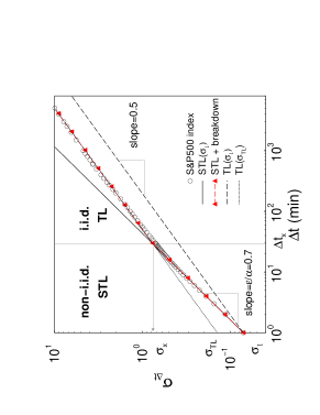
FIG. 1.: The $S\&P500$ index shows two regimes of scaling behavior for the standard deviation $\sigma$. The correlated (superdiffusive) regime at small ${\Delta t}$ corresponds to the STL process with slope $\epsilon/\alpha=0.7$. To account for the crossover to uncorrelated (normal diffusion) regime, we introduce a breakdown in the scaling for the STL process: $\lambda_{\Delta t}\equiv\lambda_{\times}=const$ and $A_{\Delta t}\equiv({\Delta t})A_{\times}$ for $\Delta t>(\Delta t)_{\times}$. The breakdown in the STL is equivalent to a transition to a TL process at large time scales. This TL process corresponds to an initial $\sigma_{TL}$ larger than the empirical $\sigma_{1}$. This is the reason for the delay (at time scale $(\Delta t)_{s}\approx 10^{3}$) in the transition from Lévy to Gaussian behavior observed for ${\cal P}_{\Delta t}(0)$ [Fig.2]. Note, that the TL process with an initial standard deviation $\sigma_{1}$ (as observed in the data) would exhibit for ${\cal P}_{\Delta t}(0)$ a transition from Lévy to Gaussian at shorter time scales.

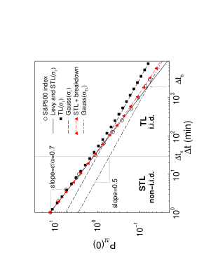
FIG. 2.: $S\&P500$ data for the probability of return to the origin ${\cal P}_{\Delta t}(0)$ mimics Lévy scaling for more than 3 decades in ${\Delta t}$. The slope and the intercept of the straight line which represents the scaling of the Lévy distribution are determined from the parameters $\alpha=1.43$ and $A_{1}=0.0014$ by fitting the initial PDF ${\cal P}_{1}(z)$ for the $S\&P500$ index. From the same fit, we obtain $\lambda_{1}=0.7$. These initial parameters are used to define the STL process. As expected, the STL process follows the Lévy scaling for ${\cal P}_{\Delta t}(0)$ at all time scales. The TL process (with $\sigma_{1}=0.07$, identical to the empirical value) exhibits a transition at short time scales to the Gaussian process (with the same value of $\sigma_{1}$), in disagreement with the data. The STL process with a breakdown at $(\Delta t)_{\times}$, however, is in agreement with the data and explains the delayed transition (at $(\Delta t)_{s}\approx 10^{3}$) to the Gaussian observed in the data.

FIG. 3.: $S\&P500$ probability distributions ${\cal P}_{\Delta t}(z)$ of price fluctuations $z$ for different time scales $\Delta t$. With solid lines, we show the PDF of the STL, with breakdown process for the same time scales and parameters used in Fig.2. Good agreement between data and the theoretical PDFs is observed for the central part. To reproduce better the experimentally observed change in slope of the far tails we use $\alpha=1.43$, $A_{1}=0.0028$, and $\lambda_{1}=2.6$. The shape of ${\cal P}_{\Delta t}(z)$ changes as a function of $\Delta t$ from exponential-like (for small $\Delta t$ — STL non-i.i.d. regime) to Gaussian-like profile of the tails (for large $\Delta t$ — TL i.i.d. regime).

FIG. 4.: For the $S\&P500$ index (Jan ’84- Dec ’95), we show how the standard deviation of price fluctuations and rates of return completely overlap, after rescaling by the average price for that period. Note, that the standard deviation is calculated for a long period of time (12 years) and for data at either high frequency (1 min) or low frequency (1 trading week). In (b) and (c) we show how the probability distributions of the same stochastic variables collapse after rescaling by the same average price. The collapse is obtained again for both low and high frequency data. We also subdivide the 12 year period in two equal subintervals, and find the same collapse.

REFERENCES

- [1] P. Lévy, Theorie de l’Addition des Variables Aléatories (Gauthier-Villars, Paris, 1937).
- [2] M. F. Shlesinger, G. M. Zaslavsky, and J. Klafter, Nature 363, 31 (1993).
- [3] T. H. Solomon, E. R. Weeks, and H. L. Swinney, Phys. Rev. Lett. 71, 3975 (1993).
- [4] A. Ott, J.-P. Bouchaud, D. Langevin, and W. Urbach, Ibid. 65, 2201 (1990).
- [5] F. Bardou, J.-P. Bouchaud, O. Emile, A Aspect, and C. Cohen-Tannoudji, Ibid. 72, 203 (1994).
- [6] F. Hayot and L. Wagner, Phys. Rev. E 49, 470 (1994); F. Hayot, Phys. Rev. A 43, 806 (1991).
- [7] J. Moon and H. Nakanishi, Phys. Rev. A 42, 3221 (1990).
- [8] G. Zumofen and J. Klafter, Chem. Phys. Lett. 219, 303 (1994).
- [9] M. Orrit and J. Bernard, Phys. Rev. Lett. 65, 2716 (1990).
- [10] R.N. Mantegna and H.E. Stanley, Phys. Rev. Lett. 73, 2946 (1994).
- [11] R. N. Mantegna and H. E. Stanley, Nature 376, 46 (1995).
- [12] I. Koponen, Phys. Rev. E 52, 1197 (1995).
- [13] For the probability function corresponds to Lévy distribution.
- [14] Different types of smooth truncation can be reproduced with changing values of : (i) for we have stretched exponential tails; (ii) for we have an exponential truncation (the case of [12]); (iii) we have process faster than exponential; and (iv) for we have Gaussian behavior.
- [15] B. V. Gnedenko and A. N. Kolmogorov, Limit Distributions for Sums of Independent Random Variables (Addison-Wesley, Cambridge, MA, 1954).
- [16] In the case of TL process, Lévy-type scaling transformations for the stochastic variable and the parameter — and — ensure scale invariant behavior only for the central profile of .
- [17] Note that the STL process characterized by given can scale with any scaling exponent in contrast to the Lévy stable process which scales with the scaling exponent . The parameter controls the dynamics of the process — probability distributions characterized with the same can exhibit different scaling behavior for different values of . E.g. for and under the transformations of Eqs. (2) the probability density scales as the Lévy stable process.
- [18] We obtain the following analytic expression: , where is the Lévy PDF [12].