Various Spin Phases from Lightly-Doped Two-legged $t$-$J$ Spin Ladders

Abstract

We study two-leg spin ladder systems analytically by using a $t$-$J$ model which includes the interchain spin exchange and the interchain hopping term. The spin part is mapped to a quantum sine-Gordon model via a bosonization method that fully accounts for the phase fluctuation. The spin gap in the Luther-Emery phase evolves to gapless Luttinger liquid phases in even-ladders at certain doping concentration. This transition occurs as doping rate increases and/or the ratio of the interchain spin exchange and hopping to the intrachain couplings decreases. We also estimate the transition temperature at which the conventional electron phase can be deconfined to spinon and holon.

PACS numbers: 75.10.Jm, 71.27.+a, 71.10.Hf, 74.20.Mn

I introduction

Low-dimensional quantum magnetic systems, such as spin chains, spin ladders, and planar lattices provide very useful information about the physics of high $T_{C}$ superconductors. During the past few years, spin-ladder systems have been studied extensively by various groups[1][2][5], especially by numerical methods or by mean-field (MF) calculations[3][6]. A“spin ladder” consists of parallel “chains” of magnetically bound $Cu$ atoms connected by interchain couplings (“rungs”), as found in $Sr_{n-1}Cu_{n+1}O_{2n}$, $La_{4+4n}Cu_{8+2n}O_{14+8n}$ (Fig. 1). Spin ladder compounds may become superconductors if doped with charge carriers[8][9]. Recently, superconductivity has been found in $Sr_{14-x}Ca_{x}Cu_{24}O_{41}$[7] below 12 K and with external pressure of 3 GPa.

Beginning with the half-filled ground state of a spin liquid, short-range singlets are formed predominantly across the rungs of the ladders from the antiferromagnetic (AF) states. The unusual spin-liquid nature of an undoped parent system and the evolution of the finite gap upon doping have also been studied by numerical methods [10]. Excitations of the singlet ground state yield spin triplets which propagate along the ladder direction. The study of even-leg ladder systems has shown that spin gaps decrease as the number of legs increase. ( The gap remains finite down to $J_{\perp}=J_{\parallel}$, which is a signature of superconductivity[11]). Within the mean-field theory, in numerical works and renormalization group (RG) calculations, a superconducting phase with a d-wave nature emerges from the short-range RVB liquid upon doping. Then, new quasiparticle (QP) states appear which carry both charge (positive) and spin.

In the weak-coupling approach, one starts with two non-interacting spin chains and turns on perturbative interchain interactions. For finite interchain interactions, this method does not accurately describe the correlations near the phase transitions. Zhang et al.[12] have studied two-leg $t-J$ ladders without the interchain exchange by mapping the spin part to a sine-Gordon model. Our study includes the spin exchange interaction across the rungs of the spin ladders and is based on a (nearly) exactly solvable model. Based on the soliton description, we discuss the phases and possible transitions between them. Exactly solving for spin ladders gives better understanding of the correlations between phase excitations and topological defects, while comparing with some weak-coupling studies[4] and MF results which partly addressed this issue[14].

We use a $t$-$J$ model for two-leg ladders in the strongly(isotropically) coupled regime in which the interchain interactions ($t_{\perp}$, $J_{\perp}$) are larger(equal) than the intrachain interactions $(t_{\parallel},J_{\parallel})$. Introducing weak coupling between two-leg ladders is staightforward for even-leg ladder systems. Recent studies[13] have shown that ladder systems with an odd number of legs are conducting Luttinger liquids in the odd-parity channel and spin liquids in the even parity channel[14]. Odd-legged ladders can be mapped to a single-chain system while even-legged ladders are equivalent to a double-chain ladder.

II the model

An effective model for the $t$-$J$ Hamiltonian is obtained as follows :

$$H = -t_{\parallel}\sum_{l=1,2}\sum_{<ij>,\sigma}(C_{li\sigma}^{+}C_{lj\sigma}+h.c.)$$ (1)

$$- t_{\perp}\sum_{l,l^{\prime}=1,2}\sum_{<ij>,\sigma}(C_{li\sigma}^{+}C_{l^{\prime}i\sigma}+h.c.)$$ (2)

$$+ J_{\parallel}\sum_{l=1,2}\sum_{<ij>,\sigma}(S_{li\sigma}S_{lj\sigma}-{1\over 4}n_{li\sigma}n_{lj\sigma})$$ (3)

$$+ J_{\perp}\sum_{l,l^{\prime}=1,2}\sum_{<ij>,\sigma}(S_{li\sigma}S_{l^{\prime}i\sigma}-{1\over 4}n_{li\sigma}n_{l^{\prime}i\sigma})$$ (4)

$$+ \mu\sum_{l=1,2}\sum_{\sigma}C_{li\sigma}^{+}C_{li\sigma}$$ (5)

where $<ij>$ is for nearest-neighbor( $j=i+1$) interactions, $l$ is the leg index and $\sigma$ is the spin $(\uparrow\downarrow)$ index. In strongly coupled $t$-$J$ models with a large Coulomb repulsion (large $U/t$ and large $J_{\perp}/J_{\parallel})$, we impose the single-occupancy constraint $\sum_{\sigma}C_{i\sigma}^{+}C_{i\sigma}=0\hskip 8.5359ptor\hskip 8.5359pt1$ at each site. The electron chemical potential $\mu$ is added for the constraint in the form of a Lagrange multiplier. The charge(hole) concentration is related to $\mu(1-\delta)={1/({1+e^{-\beta\mu}}})$. In order to study the spin part and the charge part separately, we write the electron operator as the product of a charge carrying holon $h_{i}$ and a pseudospin operator $S_{i}$: $C_{i\downarrow}=Ph_{i}S_{i}^{+}P^{+}\equiv h_{i}S_{i}^{+},\hskip 2.84544ptC_{i\uparrow}=Ph_{i}S_{i}^{-}P^{+}\equiv h_{i}S_{i}^{-}.$ The projection operator $P=(1-n_{i,-\sigma})$ reduces the four on-site states $|0,\uparrow>,|0,\downarrow>,|1,\uparrow>$ and $|1,\downarrow>$ to the physical Hilbert spaces $|hole>,|\uparrow>$ and $|\downarrow>$, thereby imposing single-occupancy at each site. Since the charge sum rule $(\sum_{\sigma}C_{i\sigma}^{+}C_{i\sigma}=1-\delta)$ holds when the projection operators are neglected, we equate the electron operator with $h\bigotimes S$. The pseudospin operators acting at site $i$ turn into spinless fermion operators $a$ via a Jordan-Wigner transformation.

III continuum limit and bosonization

In the spin exchange part, the pseudospin operators anticommute on the same site and commute on the different sites. so, we have $H(J)$ parts become $J_{\parallel}\sum_{i=1}^{N}(S_{i}^{+}S_{i+1}^{-}+h.c.)$ and $J_{\perp}\sum_{i,l}(S_{i,l}^{+}S_{i,l+1}^{-}+h.c.)$. From Jordan-Wigner transformation, the intrachain term $S_{i}^{+}S_{i+1}^{-}=a_{i}^{+}\exp[-i\pi a_{i}^{+}a_{i}]a_{i+1}=a_{i}^{+}(1-2a_{i}^{+}a_{i})a_{i+1}$ for spin $1\over 2$-system, while the interchain term $S_{i,l}^{+}S_{i,l+1}^{-}=a_{i,l}^{+}a_{,i,l+1}-2a_{i,l}^{+}a_{i,l}^{+}a_{i,l}a_{i,l+1}$. We introduce spinor fields $\phi_{\alpha}$ for the slowly-varying field $\widetilde{a_{i}}=a_{i}/i^{n}$ where $\alpha$=even at even(2s) site $i$ and odd at odd(2s+1) site $i$. The even-site and odd site are coupled by nearest-neighbor interaction, yielding $\sum_{i=1}^{N}\widetilde{a}_{i}^{+}\widetilde{a}_{i+1}=\sum_{s=0}^{N\over 2}[\phi_{e}^{+}(2s)\{\phi_{o}(2s+1)-\phi_{o}(2s-1)\}+\phi_{o}^{+}(2s+1)\{\phi_{e}(2s)-\phi_{e}(2s-2)\}]$. In continuum, the fermion field is given $\phi_{\alpha}(s)=\sqrt{2a_{0}}\Psi_{\alpha}(x)$ where $x=2sa_{0}$ with the lattice constant $a_{0}$. Then, $\phi_{o}(2s+1)-\phi_{o}(2s-1)\approx 2a_{0}\sqrt{2a_{0}}\partial_{x}\Psi_{0}(x)$. The commutation relations are $\{\Psi_{\alpha}(x),\Psi_{\beta}(y)\}=\delta_{\alpha\beta}\delta(x-y)$ and $\{\phi_{\alpha}(n),\phi_{\beta}(n\prime)\}=\delta_{\alpha\beta}\delta_{nn\prime}$. With the relation for exponentiated operators $e^{A}e^{B}=e^{[A+B]}\hskip 2.84544pte^{-[A,B]/2}=e^{B}\hskip 2.84544pte^{A}\hskip 2.84544pte^{-[A,B]}$ , we map the spin exchange interaction terms

$$J_{\parallel} \sum_{<ij>,\sigma}S_{i\sigma}S_{j\sigma}=J_{\parallel}(S_{i}^{+}S_{j}^{-}+S_{i}^{-}S_{j}^{+}+S_{iz}S_{jz})$$ (6)

$$= J_{\parallel}(\widetilde{a}_{i}^{+}\widetilde{a}_{i+1}-2\widetilde{a}_{i}^{+}\widetilde{a}_{i}^{+}\widetilde{a}_{i}\widetilde{a}_{i+1}+h.c.)\equiv H(J_{\parallel}).$$ (7)

Now the intrachain spin exchange part of Hamiltonian becomes

$$H (J_{\parallel})=2a_{0}J_{\parallel}\int dx$$ (8)

$$[ \Psi^{+}_{\eta}(x)i\sigma^{1}\partial_{x}\Psi_{\eta}(x)+\Psi^{+}_{\eta}(x)\Psi_{\eta}(x)\Psi^{+}_{\eta}(x)i\sigma^{1}\partial_{x}\Psi_{\eta}(x)]$$ (9)

where $\Psi_{\eta}$ is the Fermi field of two species(bonding, anti-bonding band) and $\sigma^{1}$ is the Pauli matrix.

Then, we bosonize the Fermi field with phase fluctuation parameters which can vary depending on the interactions (rather than the parameter being a constant $\sqrt{4\pi}$). Employing the operator expansion of the Fermi field[15], $\Psi_{\eta}(x)=\exp[i\alpha\phi_{\eta}(x)]\exp[i\beta\int_{-\infty}^{x}dy\partial_{0}\phi_{\eta}(y_{0},y)]$ where the Bose field $\phi$ and its canonical conjugate momentum $\Pi=\partial_{0}\phi$ satisfy $[\phi(x),\Pi(x^{\prime})]=i\delta(x-x^{\prime})$ and $[\Pi(x),\partial_{0}\phi(x^{\prime})]={i\over\pi}\partial_{x}\delta(x-x^{\prime})$. In order to satisfy the commutation relation of $\Psi_{\eta}(x)$, the phase fluctuation parameters $\alpha$ and $\beta$ are related as $2\alpha\beta=\pm\pi$. The Fourier components of density operators $\rho_{\eta}(q)=\sum_{k}\Psi_{\eta}^{+}(k+q)\Psi_{\eta}(k)$ satisfy the boson commutation relation $[\rho_{R}(q),\rho_{R}(-q\prime)]={-L\over 2\pi}q\hskip 2.84544pt\delta_{qq\prime}$, $[\rho_{L}(q),\rho_{L}(-q\prime)]={L\over 2\pi}q\hskip 2.84544pt\delta_{qq\prime}$ and $[\rho_{R}(q),\rho_{L}(-q\prime)]=0$, where $\rho_{R\eta}(x)-\rho_{L\eta}(x)=\Pi_{\eta}$ and $\rho_{R\eta}(x)+\rho_{L\eta}(x)={-1\over\pi}\partial_{x}\phi_{\eta}$ is the fermion density deviation from its average. Introducing the dual field $\int_{-\infty}^{x}dy\Pi_{\eta}(y)={1\over\pi}\theta_{\eta}(x)$ and linearizing the four branches of the spectrum near the Fermi surface($\pm k_{F}$), $\Psi_{\eta}(x)=e^{ik_{F}x}R_{\eta}(x)+e^{-ik_{F}x}L_{\eta}(x)$ with the right-going (R) and left-going (L) components for each specie,

$$R_{\eta}(x) = {1\over\sqrt{2\pi a_{0}}}F_{\eta}\hskip 2.84544pt\exp[-i(\theta_{\eta}(x)-\phi_{\eta}(x))],$$ (10)

$$L_{\eta}(x) = {1\over\sqrt{2\pi a_{0}}}F_{\eta}\hskip 2.84544pt\exp[-i(\theta_{\eta}(x)+\phi_{\eta}(x))]$$ (11)

where the Klein factors $F_{\eta}=\exp[-i\theta_{\eta}]$ are ladder operators[16][17], raising/lowering the $\eta$-fermion number by one. They are taken to yield the same signs for the species($\eta$) thus ignored in the thermodynamic limit, since the transverse hopping and spin exchange lead to interchain pair fluctuations[4] with both specie participating. Also, the $\Psi$ fields are written as even $\Psi_{e\eta}={1\over\sqrt{2}}(R_{\eta}+L_{\eta})$ and odd $\Psi_{o\eta}={1\over\sqrt{2}}(-R_{\eta}+L_{\eta})$. Resultantly, the intrachain exchange $J_{\parallel}$ maps to the form of $(\partial_{\mu}\phi_{\eta})^{2}+2cos({\beta\over 2}\phi_{\eta})$.

From the quartic interchain exchange $J_{\perp}$ part of Hamiltonian, $-2J_{\perp}a_{i,l}^{+}a_{i,l}^{+}a_{i,l}a_{i,l+1}=$

$$-2iJ_{\perp}(2a_{0})^{2}[\Psi_{l,e}^{+}\Psi_{l,e}\Psi_{l,e}^{+}\partial_{x}\Psi_{l+1,e}+\Psi_{l,o}^{+}\Psi_{l,o}\Psi_{l,o}^{+}\partial_{x}\Psi_{l+1,o}]$$ (12)

There are actually ten terms giving non-zero contribution to the resultant sine-Gordon, three of which are shown below.

$$H (J_{\perp})=-J_{\perp}\sum_{i,\sigma}S_{1i\sigma}S_{2i\sigma}=-2J_{\perp}a_{0}\int dx$$ (13)

$$[ L_{1}^{+}\partial_{x}{R_{2}}-R_{1}^{+}{L_{1}}R_{1}^{+}\partial_{x}{L_{2}}+{R_{2}}^{+}L_{2}L_{2}^{+}\partial_{x}{L_{1}}+..].$$ (14)

The terms in the integrand above break the left-right (chiral) symmetry which arises from the Umklapp scattering between different chains (and backscattering between opposite spins). The interchain hopping term $H(t_{\perp})=-t_{\perp}\sum_{i\sigma}(C_{1i\sigma}^{+}C_{2i\sigma}+H.C.)$ yields identical forms in which we put the intrachain charge hopping OP $h_{l,i}^{+}h_{l,i+1}=\alpha\delta\equiv\delta_{\parallel}$ where $0<\alpha<1$ and interchain OP $h_{l,i}^{+}h_{l+1,i}=\delta[1+{t_{\parallel}\over t_{\perp}}(1-\alpha)]\equiv\delta_{\perp}$. Actual values of $\alpha$, $\delta_{\perp}$, $\delta_{\parallel}$ and above rates depend on the interaction strengths $t_{\perp}$, $t_{\parallel}$.

Thus, the spin part of the Hamiltonian collected from the intrachain and the interchain contributions is

$$H_{s}=\int dx\hskip 5.69046pt{1\over{2\pi}^{2}}[\hskip 2.84544pt(\partial_{\mu}^{2}{\widetilde{\phi}_{1}}+\partial_{\mu}^{2}{\widetilde{\phi}_{2}})+Wcos({\beta\over 2})({\widetilde{\phi}_{1}}+{\widetilde{\phi}_{2}})]$$ (15)

where ${\widetilde{\phi}}$ is a rescaled field from $\phi=(1+2W\pi)\widetilde{\phi}$ with the lattice constant $a_{0}=1$. This is a quantum sine-Gordon equation which is the equation of motion of solitons (which are magnons with spin 1 (charge 0) made of two spinons bound by a confining potential).

IV phase fluctuation and the interaction strengths

The constant prefactor is the ratio of interaction strengths interchain to intrachain

$$W={\delta_{\perp}t_{\perp}-J_{\perp}\over(\delta_{\parallel}t_{\parallel}-J_{\parallel})}$$ (16)

and is related to the phase fluctuation parameter $\beta^{2}=16\pi/(1+2W)$. In case of frustrated AF (which may occur in the ground state of odd-legged ladders), the sine-Gordon equation simplifies to $H={1\over{2\pi}^{2}}\hskip 2.84544pt[(\partial_{\mu}{\widetilde{\phi}})^{2}+W\hskip 2.84544ptcos(\beta\widetilde{\phi})]$. For any finite value of $\beta$, the system has a zero-point fluctuation, In the dilute-soliton limit, the quantum fluctuation is dominated by the hard-core interaction between the spinless fermions[16]. Depending on the parameter $\beta$ or $W$, we have various soliton phases : (1) $W={J_{\perp}\over J_{\parallel}}\equiv W_{0}$ : This is undoped state whose ground state is a AF spin liquid, as known from existing numerical studies[11]. (2)$W\geq W_{0}$ : Here we have Luther-Emery liquid with the gapped spinon(soliton) and gapless charge excitations. In the lower-temperature regime, excitonic soliton-antisoliton bound states exist. These correspond to integer spin magnon states which are bound states of two spin-$1\over 2$ spinons. The CDW inherited from chains exists as well as the Luttinger liquid phase holons. When temperature increases, the excitonic bound states can be broken to spin-triplets ($S=1$ magnon)which make the system spin-gap metal. (3) ${1\over 2}<W<W_{0}$ : In this case, repulsive interaction between spinons exists, and there are no stable solitons. This is equivalent to the strong fluctuation of a gauge field. SDW is in the background. (4) $0<W\leq{1\over 2}$ : The spinons are a Luttinger liquid as shown in algebraically decaying spin-spin correlation given below. The charge part is a Luttinger liquid as in (2). (5) $W=0$ or $\delta_{\perp}J_{\perp}=t_{\perp}$ : This limit corresponds to single soliton(spinon gas) mode. (6)$W=\infty$ or $\delta_{\parallel}J_{\parallel}=t_{\parallel}$ : This corresponds to the classical limit with a finite soliton density. The electron states have dimensional crossovers from the incommensurate 1D regime for $W<{1\over 2}$ to commensurate 2D-like states for $W_{0}<W$. At low doping and at low temperatures, the system can develop superconducting channel[10]. An excited spin phase generates magnons from triplets and solitons which propagate in the background of spin-density-wave(SDW). Weak but finite anisotropy or spontaneous breaking of chiral symmetry cause spin stiffness and low-energy excitations. The interplay of the excitation modes, such as order-preserving collective magnons and order-destroying topological solitons, may possibly lead to some long-range or intermediate-range order. Considering the asymptotic behaviours shown from scaling equations (Appendix), a schematic phase diagram is given in Fig. 2, which shows the various spinon and electron phases with the parameter $W$.

V charge part

The separated charge part of the Hamiltonian is diagonalized via a Bogoliubov transformation of the holon operators. $H=\sum_{k}E_{k}(f_{k}^{+}f_{k}+\rm constants)$ where the holon excitation spectrum $E_{k}=-2t_{\parallel}cos\hskip 2.84544ptk{+\atop-}{\delta_{\perp}}t_{\perp}$ is valid for $t_{\perp}\geq t_{\parallel}(1-cos\hskip 2.84544pt2\delta\pi)$ from the Luttinger sum rule. The charge phase with gapless excitation forms a Tomonaga-Luttinger ground state. According to numerical works [18][11], holes have lower energies when they form pairs across the rungs of the ladders. Thus, low-energy excitations include hole-hole pairs and hole-spin bound states (with positive charge) propagating along the ladder with a kinetic energy of about $4t_{\parallel}^{2}/J_{\perp}$. These excitations as well as the fluctuations of hole pairs move against the lowest-energy background of charge-density wave(CDW). The holon speed is $v_{h}=2t_{\parallel}sin\delta\pi$.

VI correlations

The asymptotic electron Green’s function can be calculated from perturbation theory excluding the vertex corrections[19][20] and is given by

$$G_{e}\approx{e^{i2k_{F}x}\over(x^{2}-v_{s}^{2}t^{2})^{\gamma}(x-v_{h}t)^{\eta}(x+v_{h}t)^{\eta}}$$ (17)

where $\gamma=({\sqrt{1+W^{2}}-1)/2}$ with a spinon velocity $v_{s}=v_{F}\equiv 1$ and $\eta=1/2$. The propagator $G_{e}$ can be determined by convoluting the holon propagator and the spinon propagator and has no simple poles for low-energy states. Thus, the Fermi surfaces are considered separately for the holon and for the spinon. The size of the holon Fermi surface is found from $\sum_{k,\omega}G_{h}(k,\omega)=\delta$ ($\delta$ being the doping concentration). The ground state of the half-filled insulator is a disordered (or dimerized) spin liquid made of spin singlets. These singlets which form across the rungs become spin triplets as they are excited. Also, the triplets can propagate along the ladder as well as along the chain. The propagation ${\it across}$ the rungs and ladders are “incoherent” in the sense that there is no stable eigenstate for the electron. The quantum numbers, such as spin, charge, and momentum, are not the same throughout the propagation from one leg to another[21]. As separated phase fields, the charge and the spin degrees of freedom propagate with different speeds. At small lengths, the phase separation may manifest itself spatially in real space, for example as striped phases, as discussed by some authors[22]. To see whether there is any strong-coupled fixed point, consider turning off the interchain hopping $t_{\perp}$. The renormalization group(RG) dimension of the wavefunction comes from rescaling the variables $(x,y,t)\rightarrow(\alpha x,y,\alpha t)$. From the propagator, we have $\psi\rightarrow\alpha^{-{1\over 2}-\eta}$. So, the Hamiltonian $H_{\perp}$ has the RG dimension of ${1\over 2}+\eta$. The interchain hopping is irrelevant and the Luttinger liquid becomes a fixed point, if and only if $\eta>{1\over 2}$. This corresponds to the case of interchain interactions being much weaker than intrachain ones ($t_{\perp}\gg t_{\parallel}$). However, in strongly coupled ladders, $J_{\perp}/J_{\parallel}$ remains sufficiently large to develop gaps[23][24] and RG flow is away from the unstable Luttinger liquid fixed point[4]. Given that $t_{\perp}$ is greater than the spin gap, there is no strong-coupled fixed point, for even-legged ladders($\eta\leq{1\over 2})$. The equal-time spin-spin correlation is a power-law form

$$<S(r)S(0)>\approx x^{-\sqrt{1+W^{2}}}\hskip 2.84544ptcos\hskip 2.84544pt2k_{F}x,$$ (18)

which shows the spinons being a non-Fermi liquid. From second-order perturbation theory[25], the spin gap size is $J_{\perp}+J_{\parallel}cos\hskip 2.84544ptk_{\parallel}+{1\over 4}J^{2}_{\parallel}/J_{\perp}(3-cos\hskip 2.84544pt2k_{\parallel})$ with $k_{\parallel}=\pi$.

VII deconfinement

In the 2D AF Heisenberg model or $CP^{1}$ model, deconfinement of the electron (to a holon and spinon) occurs at $T=0$[26]. As for spin-ladder systems, the “electron” phase is realized by having the spin and the charge phases confined at finite $T$ above the transition temperature $T_{CD}$. Since the confinement-deconfinement(CD) transition occurs in the absence of ordering, it is like a Kosterlitz-Thouless transition occuring in (2+1) dimensional system. From the partition function, $T_{CD}$ is found

$${\delta_{\parallel}t_{\parallel}-J_{\parallel}\over 2k[\delta_{\perp}t_{\perp}-J_{\perp}]}<T_{CD}<{\delta_{\parallel}t_{\parallel}-J_{\parallel}\over k[\delta_{\perp}t_{\perp}-J_{\perp}]}$$ (19)

where $k$ is Boltzmann constant. Hence, for $T>T_{CD}$, the electron propagator has the product form $G_{s}(r,t)*G_{h}(-r,-t)$. Below $T_{CD}$, the spin phase and the charge phase are separated due to the screening of the confining potential between holons and spinons. Spin-charge separation is a well-accepted fact for 1D systems which are Luttinger liquids. Spin ladders make transition, at some doping rates $\delta$, to a Luttinger liquid phase, where both spin and charge excitations become gapless.

In summary, we map the spinons to solitons which are either magnons (excitons when bound) or excited phasons. From the soliton gap, we have the spin-gapped mode while the charge part is gapless Luttinger liquid. As the doping increases the ladders can develop superconducting phase or lose the spin gap beyond certain hole concentration. Also, depending on the ratio of interchain couplings to intraleg interactions, the spin ladders can become gapless Luttinger liquid. Our phase diagram is consistent with the features found in MF studies or weak-coupling approaches, such as presence of gapless mode and superconducting phase from even-ladders. The comprehensive diagram shows possible transitions as an explicit function of coupling ratio and doping. The electron propagator and the spin-spin correlation obey power-laws with the exponents depending on the interaction strengths and the doping rate. This shows the correlation of topological defects and phase excitations. Constructive interferences of phase excitations (solitons and magnons) may lead to the formation of intermediate-range or long range order, which is our forthcoming study. The electron is seen as a confined phase of the gauge flux associated with each point. Below the estimated transition temperature, the spin phase and the charge phase are separated. Henceforth, even-ladders show the crossover from gapped 2D-like states to gapless 1D-nature, depending on the interleg couplings and/or the doping rate.

A renormalization group equations

Following Fabrizio[4], Kishine[27] and Bourbonnais[28], we investigate the aymptotic behaviours in/around the gapped phase by RG flow of the couplings. The partition function $Z=\int De^{S}$ where the action consists of one-particle hopping process $S_{(1)}$ and two-particle scattering $S_{(2)}$ in the ladder, $S=S_{(1)}+S_{(2)}$. The dispersion is linearized with respect to the bonding(B) and anti-bonding(A) band which lie above(inner) the bonding band(LB, LA, RA, RB), where $L$, $R$ denote the right-moving, left-moving fields. Each band ranges by the bandwidth cutoff $K_{0}$. The interladder repulsion generates scattering vertices of Fig. 3. The action for the one-particle process is given

$$S_{(1)}=\sum_{K,\sigma}\sum_{\eta=A,B}[G^{-1}_{L\eta}(K_{\parallel})L^{+}_{\eta\sigma}(K)L_{\eta\sigma}(K)+G^{-1}_{R\eta}(K_{\parallel})R^{+}_{\eta\sigma}(K)R_{\eta\sigma}(K)$$ (A1)

where $K=(k_{\parallel},k_{\perp},i\epsilon)$, $K_{\parallel}=(k_{\parallel},i\epsilon)$ with the fermion frequency $\epsilon_{n}=(2n+1)\pi\beta$, and the Green’s functions are $G_{L\eta}=[i\epsilon_{\eta}+v_{F}(k_{\parallel}+k_{F\eta})]^{-1}$, $G_{R\eta}=[i\epsilon_{\eta}-v_{F}(k_{\parallel}-k_{F\eta})]^{-1}$, with the Fermi momenta of the anti-bonding band $k_{FA}=k_{F}-t_{\perp}/v_{F}$ and of the bonding band $k_{FB}=k_{F}+t_{\perp}/v_{F}$. The action for the two-particle processes is given

$$S_{(2)} = {2\pi v_{F}\over\beta}\sum_{\eta,K,\sigma}[g_{0}(\sigma_{1}\sigma_{2}\sigma_{3}\sigma_{4})L^{+}_{\eta\sigma_{1}}(K_{1})R^{+}_{\eta\sigma_{2}}(K_{2})R_{\eta\sigma_{3}}(K_{3})L_{\eta\sigma_{4}}(K_{4})\delta(K_{1}+K_{2}-K_{3}-K_{4})$$ (A2)

$$+ g_{f}(\sigma_{1}\sigma_{2}\sigma_{3}\sigma_{4})L^{+}_{\eta\sigma_{1}}(K_{1})R^{+}_{\eta\prime\sigma_{2}}(K_{2})R_{\eta\prime\sigma_{3}}(K_{3})L_{\eta\sigma_{4}}(K_{4})\delta(K_{1}+K_{2}-K_{3}-K_{4})$$ (A3)

$$+ g_{b}(\sigma_{1}\sigma_{2}\sigma_{3}\sigma_{4})L^{+}_{\eta\sigma_{1}}(K_{1})R^{+}_{\eta\prime\sigma_{2}}(K_{2})L_{\eta\sigma_{3}}(K_{3})R_{\eta\prime\sigma_{4}}(K_{4})\delta(K_{1}+K_{2}-K_{3}-K_{4})$$ (A4)

$$+ g_{t}(\sigma_{1}\sigma_{2}\sigma_{3}\sigma_{4})L^{+}_{\eta\sigma_{1}}(K_{1})R^{+}_{\eta\sigma_{2}}(K_{2})R_{\eta\prime\sigma_{3}}(K_{3})L_{\eta\prime\sigma_{4}}(K_{4})\delta(K_{1}+K_{2}-K_{3}-K_{4})]$$ (A5)

where the dimensionless couplings $g(\sigma_{1}\sigma_{2}\sigma_{3}\sigma_{4})=g^{(b)}\delta(\sigma_{1}\sigma_{3})\delta(\sigma_{2}\sigma_{4})-g^{(f)}\delta(\sigma_{1}\sigma_{3})\delta(\sigma_{2}\sigma_{4})$ and $g_{0}$ is for the intraband process, $g_{f}$ for interband forward scattering, $g_{b}$ for interband backward scattering, $g_{t}$ for interband tunneling. We scale the two-spin processes to remove the high-energy components, by parametrizing the bandwidth cutoff $K(l)=K_{0}e^{-l}$ with length $l$. The scaling equations for the scattering vertices are from ${d\ln{g_{\alpha}}^{i}(l)\over dl}=z_{\alpha}^{i}(l)-2z(l)$ where $i=b$ for backward scattering and $i=f$ for forward scattering. The vertex correction diagrams to the second order of the couplings($Z_{\alpha}^{i}(l)$) are shown in Fig. 4. The linearized bands consist of the slow modes(s) (from the central portions of the branches) and the fast modes(f) (from the outer edges). The action is decomposed $S_{(1),s}+S_{(2),s}+S_{(1),f}+S_{(2),f}$. Expanding the fast components $\exp[S_{(1),f}+S_{(2),f}]$ with respect to $S_{(2),f}$ and integrating out with the fast modes over $dK(l)={1\over 2}K(l)dl$, the partition function becomes $Z=\int D_{s}{\exp[S_{(1),s}+S_{(2),s}+\sum^{\infty}_{l=0}{1\over l!}<<S_{(2),f}^{l}>>_{c}}]$ where $<<>>_{c}$ denotes the connected diagram. The renormalized propagator and hopping amplitudes give renormalized action.

$$\widetilde{G}^{-1}_{\alpha\eta}(K_{\parallel})=[1+z(l)dl+\cal{O}\rm{(dl^{2})}]G^{-1}_{\alpha\eta}(K)$$ (A6)

$$\widetilde{g}^{i}_{\alpha}=[1+z^{i}_{\alpha}(l)dl+\cal{O}\rm{(dl^{2})}]g^{i}_{\alpha}$$ (A7)

$$\widetilde{t_{\perp}}=[1+\cal{O}\rm{(dl^{2})}]]t_{\perp}$$ (A8)

where $\alpha$ stand for (o, f, b, t) and $i$ for backward(1) and forward(2) scatterings. The Feynman diagrams contributing to the order $dl$ are evaluated. Those in Fig. 4 give $z^{i}_{\alpha}(l)$, while the self-energy diagrams give $z(l)$ of the scaling equations (Fig. 5).

$$z(l) = g^{(1)}_{0}(l)^{2}+g^{(2)}_{0}(l)^{2}+g^{(1)}_{f}(l)^{2}+g^{(2)}_{f}(l)^{2}+g^{(1)}_{b}(l)^{2}+g^{(2)}_{b}(l)^{2}+g^{(1)}_{t}(l)^{2}$$ (A9)

$$+ g^{(2)}_{t}(l)^{2}-g^{(1})_{0}(l)g^{(2)}_{0}(l)-g^{(1)}_{f}(l)g^{(2)}_{f}(l)-g^{(1)}_{b}(l)g^{(2)}_{b}(l)-g^{(1)}_{t}(l)g^{(2)}_{t}(l)$$ (A10)

The scaling equations follow, provided small $K_{0}<\Delta k_{F}$ ;

$${d\over dl}g^{(1)}_{0}(l) = -2(g^{(1)}_{0}(l)^{2}+g^{(1)}_{t}(l)g^{(2)}_{t}(l))+2(g^{(1)}_{f}(l)g^{(2)}_{t}(l)^{2}-g^{(1)}_{f}(l)g^{(1)}_{t}(l)g^{(2)}_{t}(l))$$ (A11)

$$- 2g^{(1)}_{0}(l)(g^{(1)}_{0}(l)^{2}+g^{(1)}_{f}(l)^{2}+g^{(1)}_{t}(l)^{2}+g^{(2)}_{t}(l)^{2}-g^{(1)}_{t}(l)g^{(2)}_{t}(l))$$ (A12)

$${d\over dl}g^{(2)}_{0}(l) = -(g^{(1)}_{0}(l)^{2}+g^{(1)}_{t}(l)^{2}+g^{(2)}_{t}(l)^{2})+2(g^{(2)}_{f}(l)g^{(2)}_{t}(l)^{2}-g^{(1)}_{t}(l)g^{(2)}_{t}(l)g^{(2)}_{f}(l))$$ (A13)

$$+ 2g^{(1)^{2}}_{t}(l)g^{(2)}_{f}(l)-g^{(1)^{3}}_{0}-g^{(1)^{2}}_{f}(l)g^{(1)}_{0}(l)-g^{(1)^{2}}_{t}(l)g^{(1)}_{f}(l)$$ (A14)

$$- 2g^{(2)}_{0}(l)(g^{(1)}_{t}(l)^{2}+g^{(2)}_{t}(l)^{2}-g^{(1)}_{t}(l)g^{(2)}_{t}(l))$$ (A15)

$${d\over dl}g^{(1)}_{f}(l) = -2(g^{(1)}_{f}(l)^{2}+g^{(1)}_{t}(l)^{2}-g^{(1)}_{t}(l)g^{(2)}_{t}(l))+2[g^{(1)}_{0}(l)g^{(2)}_{t}(l)^{2}-g^{(1)}_{0}(l)g^{(1)}_{t}(l)g^{(2)}_{t}(l)]$$ (A16)

$$- 2g^{(1)}_{f}(l)[g^{(1)}_{0}(l)^{2}+g^{(1)}_{f}(l)^{2}+g^{(1)}_{t}(l)^{2}g^{(2)}_{t}(l)^{2}-g^{(1)}_{t}(l)g^{(2)}_{t}(l)]$$ (A17)

$${d\over dl}g^{(2)}_{f}(l) = -(g^{(1)}_{f}(l)^{2}-g^{(2)}_{t}(l)^{2})+2(g^{(2)}_{0}(l)g^{(2)}_{t}(l)^{2}-g^{(1)}_{t}(l)g^{(2)}_{t}(l)g^{(2)}_{0}(l))$$ (A18)

$$+ 2g^{(1)}_{t}(l)^{2}g^{(2)}_{0}(l)-g^{(1)}_{t}(l)^{2}g^{(1)}_{0}(l)-g^{(1)}_{0}(l)^{2}g^{(1)}_{f}(l)-g^{(1)}_{f}(l)^{3}$$ (A19)

$$- 2(g^{(2)}_{f}(l)(g^{(1)}_{t}(l)^{2}+g^{(2)}_{t}(l)^{2}-g^{(1)}_{t}(l)g^{(2)}_{t}(l))$$ (A20)

$${d\over dl}g^{(1)}_{b}(l) = -2(g^{(1)}_{b}(l)g^{(2)}_{f}(l)+g^{(1)}_{f}(l)g^{(2)}_{b}(l)+g^{(1)}_{b}(l)g^{(1)}_{0}(l)-g^{(1)}_{b}(l)g^{(2)}_{0}(l)$$ (A21)

$$+ g^{(1)}_{0}(l)g^{(1)}_{b}(l)-g^{(1)}_{0}(l)g^{(2)}_{b}(l))-2g^{(1)}_{b}(l)[(g^{(2)}_{b}(l)-g^{(2)}_{f}(l))^{2}$$ (A22)

$$- g^{(1)}_{0}(l)g^{(2)}_{0}(l)+g^{(1)}_{0}(l)g^{(2)}_{f}(l)+g^{(1)}_{f}(l)g^{(2)}_{0}(l)-g^{(1)}_{f}(l)g^{(2)}_{f}(l)+g^{(1)}_{0}(l)^{2}+g^{(1)}_{f}(l)^{2}]$$ (A23)

$$+ 2g^{(1)}_{b}(l)(g^{(1)}_{t}(l)^{2}-g^{(1)}_{t}(l)g^{(2)}_{t}(l)+g^{(2)}_{t}(l)^{2})$$ (A24)

$${d\over dl}g^{(2)}_{b}(l) = -2(g^{(2)}_{b}(l)g^{(2)}_{f}(l)-g^{(2)}_{b}(l)g^{(2)}_{0}(l)+g^{(1)}_{b}(l)g^{(1)}_{f}(l))$$ (A25)

$$- 2g^{(1)}_{b}(l)g^{(1)}_{0}(l)g^{(1)}_{f}(l)-2g^{(2)}_{b}(l)[(g^{(1)}_{0}(l)-g^{(1)}_{f}(l))^{2}-g^{(1)}_{0}(l)g^{(2)}_{0}(l)$$ (A26)

$$+ g^{(1)}_{0}(l)g^{(2)}_{f}(l)+g^{(1)}_{f}(l)g^{(2)}_{0}(l)-g^{(1)}_{f}(l)g^{(2)}_{f}(l)+(g^{(2)}_{0}(l)-g^{(2)}_{f}(l))^{2}]$$ (A27)

$$- 2g^{(2)}_{b}(l)(g^{(1)}_{t}(l)^{2}-g^{(1)}_{t}(l)g^{(2)}_{t}(l)+g^{(2)}_{t}(l)^{2})$$ (A28)

$${d\over dl}g^{(1)}_{t}(l) = -2(2g^{(1)}_{t}(l)g^{(}1)_{f}(l)-g^{(1)}_{t}(l)g^{(2)}_{f}(l)-g^{(1)}_{f}(l)g^{(2)}_{t}(l)+g^{(1)}_{0}(l)g^{(2)}_{t}(l)$$ (A29)

$$+ g^{(1)}_{t}(l)g^{(2)}_{0}(l))+2(2g^{(1)}_{t}(l)g^{(2)}_{0}(l)g^{(2)}_{f}(l)-g^{(1)}_{0}(l)g^{(1)}_{t}(l)g^{(2)}_{f}(l)$$ (A30)

$$- g^{(1)}_{f}(l)g^{(1)}_{t}(l)g^{(2)}_{0}(l))-2g^{(1)}_{t}(l)(g^{(1)}_{0}(l)^{2}+g^{(2)}_{0}(l)^{2}+g^{(1)}_{f}(l)^{2}+g^{(2)}_{f}(l)^{2}$$ (A31)

$$+ g^{(1)}_{t}(l)^{2}+g^{(2)}_{t}(l)^{2}-g^{(1)}_{0}(l)g^{(2)}_{0}(l)-g^{(1)}_{f}(l)g^{(2)}_{f}(l)-g^{(1)}_{t}(l)g^{(2)}_{t}(l))$$ (A32)

$${d\over dl}g^{(2)}_{t}(l) = -2(g^{(1)}_{0}(l)g^{(1)}_{t}(l)-g^{(2)}_{0}(l)g^{(2)}_{t}(l)-g^{(2)}_{f}(l)g^{(2)}_{t}(l))$$ (A33)

$$+ 2(2g^{(2)}_{0}(l)g^{(2)}_{f}(l)g^{(2)}_{t}(l)-g^{(1)}_{f}(l)g^{(2)}_{0}(l)g^{(2)}_{t}(l)-g^{(1)}_{0}(l)g^{(2)}_{f}(l)g^{(2)}_{t}(l))$$ (A34)

$$+ 2g^{(1)}_{0}(l)g^{(1)}_{f}(l)g^{(2)}_{t}(l)-g^{(1)}_{t}(l)g^{(1)}_{f}(l)g^{(1)}_{0}(l))-2g^{(2)}_{t}(l)(g^{(1)}_{0}(l)^{2}+g^{(2)}_{0}(l)^{2}+g^{(1)}_{f}(l)^{2}$$ (A35)

$$+ g^{(2)}_{f}(l)^{2}+g^{(1)}_{t}(l)^{2}+g^{(2)}_{t}(l)^{2}-g^{(1)}_{0}(l)g^{(2)}_{0}(l)-g^{(1)}_{f}(l)g^{(2)}_{f}(l)-g^{(1)}_{t}(l)g^{(2)}_{t}(l))$$ (A36)

From the initial condition $g_{\alpha}^{(i)}(0)=t^{2}/{J\pi v_{F}}\equiv I\geq 0$, the scaling equations give the strong-coupling fixed point ; $g_{0}^{(1)}=-1$, $g_{f}^{(1)}=0$, $g_{t}^{(1)}=1$, $g_{0}^{(2)}=1/4(2I-3)$, $g_{f}^{(2)}=1/4(2I+1)$, $g_{f}^{(2)}=1$. However, the couplings actually do not flow to this fixed point, as far as the interchain hopping is greater than the gap size, since interchain pair fluctuations are dominant excitations[4]. The scale invariant coupling for the charge part is $g_{\rho,\pm}=(g^{(1)}_{0}-2g^{(2)}_{0})\pm(g^{(1)}_{f}-2g^{(2)}_{f})$. The invariant coupling for the spin part $g_{\sigma,\pm}=g^{(1)}_{0}\pm g^{(1)}_{f}$ where the $+$ sign is for the total mode and $-$ for the relative mode. From above g’s, the spin stiffness is determined $K_{\mu}=\sqrt{{1+g_{\mu}}\over{1-g_{\mu}}}$. So, $K_{\sigma,+}=0$ means that the system developed the spin gap phase, while the charge part remains gapless from $K_{\rho,\pm}=0$ (Luther-Emery phase)[29]. In our equation (8), the sine-Gordon mass term identifies $W\sim(Jv_{F}/t^{2})^{4}{g_{1}\over\sqrt{v_{F}^{2}-g_{1}^{2}}}$ where $g_{1}$ respresents some strong coupling value resulted from the scaling equations.

FIG. 1.: spin ladder example : a two-leg ladder system. The dashed circles are for spin singlets (triplets, if excited) and for holon pairs after doped.

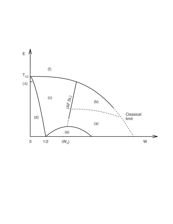
FIG. 2.: phase diagram : the energy scale vs. the ratio $W=[\delta_{\perp}t_{\perp}-J_{\perp}]/[\delta_{\parallel}t_{\parallel}-J_{\parallel}]$
“AF SL” stands for antiferromagnetic spin liquid which occurs at $W=W_{0}=J_{\perp}/J_{\parallel}$ with $\delta=0$. The spin gapsize $\Delta$ is marked for the point where gapped spinon phases branch from AF SL state. (a)gapped magnons; excitonic bound states of spinons,Luther-Emery liquid(LE) with gapless charge excitation (b) LE with gapful spinons and gapless holons, CDW (c) unstable solitons, gauge bosons, SDW (d) Luttinger liquid (paramagnetic); gapless excitations of both-charge and spin (e) superconducting (with d-wave symmetry) (f) electron phase: spinon and holon confined

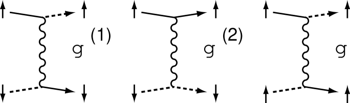
FIG. 3.: interaction vertices. The solid lines are for the right-going fermions and the dashed lines for the left-going ones. $g^{(1)}$ and $g^{(2)}$ denote backward and forward scattering couplings, respectively.

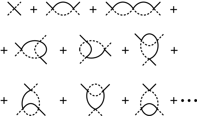
FIG. 4.: vertex diagrams to the next-to-the-leading order.

REFERENCES

• [1] S. Capponi and D. Poilblanc, Phys. Rev. B 57, 6360 (1998) and references therein.
• [2] R. Hlubina, Phys. Rev. B 50, 8252 (1994).
• [3] E. Dagotto, J. Riera and D. Scalapino, Phys. Rev. B 45, 5744 (1992).
• [4] M. Fabrizio, A. Parola and E. Tosatti, Phys. Rev. B 46, 3159 (1992), M. Fabrizio, Phys. Rev. B 48, 15838 (1993)
• [5] D. Shelton, A. Nersesyan and A. Tsvelik, Phys. Rev. B 53, 8521 (1996).
• [6] S.Β R. White and D.Β J. Scalapino, Phys. Rev. B 57, 3031 (1998).
• [7] Z. Hiroi, J. of Solid St. Chem 123, 223 (1996).
• [8] K. Kumagai, S. Tsuji, M. Kato, and Y. Koike, Phys. Rev. Lett. 78, 1992 (1997).
• [9] S. Miyakasa etΒ al., preprint (1998).
• [10] C.Β A. Hayward and D. Poiblanc, Phys. Rev. B 53, 11721 (1996).
• [11] M. Troyer, H. Tsunetsugu, and T.Β M. Rice, Phys. Rev. B 53, 251 (1996).
• [12] G.-M. Zhang, S. Feng, and L. Yu, Physical Review B 49, 9997 (1994).
• [13] T.Β M. Rice, S. Haas, M. Sigrist, and F.Β C. Zhang, Phys. Rev. B 56, 14655 (1997).
• [14] M. Sigrist, T.Β M. Rice, and F.Β C. Zhang, Phys. Rev. B 49, 12058 (1994).
• [15] E. Fradkin, Field Theories of Condensed Matter Systems, Addison-Wesley (1991).
• [16] F.Β D.Β M. Haldane, Journal of Physics. A : Math. Gen. 15, 507 (1982).
• [17] J. von Delft and H. Schoeller, cond-mat/9805275
• [18] H. Tsunetsugu, M. Troyer, and T.Β M. Rice, Phys. Rev. B 49, 16078 (1994).
• [19] X.Β G. Wen, Physical Review B 42, 6623 (1990).
• [20] A.Β M. Finkelstein and A. Larkin, Phys. Rev. B 47, 10461 (1993).
• [21] D.Β G. Clarke, S.Β P. Strong, and P.Β W. Anderson, Phys. Rev. Lett. 72, 3218 (1994).
• [22] V.Β J. Emery, S.Β A. Kivelson, and O. Zachar, Phys. Rev. B 56, 6120(1997).
• [23] D.Β V. Khveshchenko, Physical Review B 50, 380 (1994).
• [24] K. Damle and S. Sachdev, Phys. Rev. B 57, 8307 (1998).
• [25] M. Reigrotzki, H. Tsunetsugu, and T.Β M. Rice, J of Phys: Condens. Matter 6, 9235 (1994).
• [26] I. Ichinose and T. Matsui, Phys. Rev. B 51, 11860 (1995).
• [27] J. Kishine and K. Yonemitsu, J. of Phys. Soc. Jpn. 67, 1714 (1998)
• [28] C. Bourbonnais and L. G. Caron, Int. J. Mod. Phys. B 5, 1033 (1991)
• [29] H-H. Lin, L. Balents and M. P. A. Fisher, Phys. Rev. B 56, 6569 (1997)
Refer to caption