Spinodal decomposition of an ABv model alloy: Patterns at unstable surfaces

Abstract

We develop mean-field kinetic equations for a lattice gas model of a binary alloy with vacancies (ABv model) in which diffusion takes place by a vacancy mechanism. These equations are applied to the study of phase separation of finite portions of an unstable mixture immersed in a stable vapor. Due to a larger mobility of surface atoms, the most unstable modes of spinodal decomposition are localized at the vapor-mixture interface. Simulations show checkerboard-like structures at the surface or surface-directed spinodal waves. We determine the growth rates of bulk and surface modes by a linear stability analysis and deduce the relation between the parameters of the model and the structure and length scale of the surface patterns. The thickness of the surface patterns is related to the concentration fluctuations in the initial state.

I Introduction

The phase separation of alloys and other unstable mixtures (binary fluids, glasses, polymer blends) has been extensively studied for decades [1, 2, 3, 4, 5]. In a typical experiment, a stable mixture is quenched into an unstable state by a sudden change in an external control parameter, mostly temperature or pressure. Then, domains of the new equilibrium phases develop and coarsen, leading to a heterogeneous material. As the mechanical and transport properties of an alloy may depend considerably on its microstructure, the understanding of the dynamics of domain formation and growth is of great practical importance. In addition, phase separation is an interesting example of a process where spontaneous pattern formation occurs during the approach to equilibrium.

In recent years, attention has been drawn to surface effects on spinodal decomposition, mainly due to interesting experimental results on polymer blends [6, 7, 8, 9, 10, 11]. Thin films of mixture are placed between glass plates, or between a substrate and vacuum, and quenched. If the interactions with the surface favor one of the components, this component rapidly segregates to the surface and triggers phase separation in the bulk: one observes surface-directed spinodal decomposition, during which concentration waves propagate from the surface into the sample. In some of the experiments, modulations parallel to the surface are observed, leading to a pattern along the surface with a distinct length scale [7, 8, 9]. The surface effects are in competition with bulk spinodal decomposition, and only a thin layer is affected by the surface, whereas in the interior of the sample the usual bulk structures are found. Interesting questions are then what determines the type of structures found at the surface, and to predict typical length scales and growth rates of the patterns, as well as the thickness of the surface layer.

The dynamics of spinodal decomposition near planar substrates has been investigated using continuum models [12, 13, 14], Monte Carlo simulations [15], and mean-field kinetic equations [16]. On the other hand, very little is known about free surfaces, which can deform during the decomposition process [17]. We have recently found that surface modes and spinodal waves at free surfaces can be observed in a simple lattice model [18], and the present paper is devoted to a detailed study of this phenomenon.

The classical theory for the early stage of spinodal decomposition, based on out-of-equilibrium thermodynamics, was proposed by Cahn and Hilliard [1]. The Cahn-Hilliard equation is obtained by postulating that the local interdiffusion currents are proportional to the gradients of the local chemical potential, and supposing that this chemical potential can be derived from a free energy functional of Ginzburg-Landau type. The proportionality constant is the atomic mobility, which is a phenomenological parameter in this theory. For a homogeneous initial state, the Cahn-Hilliard equation may be linearized around the average composition, and analyzed in terms of Fourier modes. Long wavelength perturbations grow exponentially with time, whereas short wavelength fluctuations are damped by the gradient terms, related to the surface tension. A typical length scale of the resulting domain pattern is then given by the wavelength of the fastest growing mode.

It has been recognized that simplified lattice models are valuable tools to study the influence of microscopic dynamics on the process of phase separation in metallic alloys. They provide a convenient conceptual framework with a minimum number of parameters. Such lattice gas models assume the existence of a fixed crystal lattice, the sites of which can be occupied by the atoms of different species, or by vacancies. A configuration evolves by atomic jumps from site to site. Many studies have been carried out on the kinetic Ising model with Kawasaki spin exchange dynamics [19, 20, 21, 22, 23], which corresponds to the direct exchange of atoms. In most alloys, however, the dominant mechanism of diffusion is a vacancy mechanism [24], and several models of vacancy-mediated spinodal decomposition have been investigated [25, 26, 27, 28]. In our model, the rates for atomic jumps follow an Arrhenius law.

A standard procedure to investigate the dynamics of such models are Monte Carlo simulations [4]. The advantage of this approach is that the simulations constitute a genuine realization of the stochastic model, and all correlations in space and time are preserved. But for the same reason, an analytic understanding is difficult. Therefore, there have been numerous attempts to formulate microscopic kinetic equations which are analytically tractable. These equations are derived from the microscopic master equation by an approximation of mean-field type. While the linearized equation of Khatchaturyan [29] is valid only near equilibrium, recently several authors have proposed fully nonlinear kinetic equations for Ising and lattice gas models [30, 31, 32, 33, 34]. These equations can be cast in the form of generalized Cahn-Hilliard equations, where the atomic mobility depends explicitly on the details of the microscopic dynamics. Such equations have been applied successfully to the study of phase-separation dynamics in binary and ternary systems [35, 36, 37], and to dendritic growth [38]. In particular, kinetic equations for models with vacancy dynamics have been proposed by Chen and Geng [39] and by Puri and Sharma [40]. We will follow the approach developed by one of the present authors [32], which allows to relate the microscopic equations in a particularly straightforward manner to the equations of out-of equilibrium thermodynamics.

All the studies of vacancy-mediated phase separation we are aware of start from a homogeneous initial state. We study here the evolution of droplets of a dense mixture with few vacancies, immersed in a bath of vacancy-rich “vapor” phase. The interesting point in this situation is that we can have interfaces between an unstable mixture and a stable vapor which are “neutral”, that is without segregation of one of the components. Such interfaces are impossible in a binary model like the Ising model, where any stable phase below the critical temperature favors one of the components.

In our model, the atoms situated near the surface of the droplets have a larger mobility than bulk atoms. Therefore, phase separation is fastest at the surface. We observe different structures at the surface, depending on the model parameters and the initial composition of the mixture. In the specially symmetric case of equal interaction energies and concentrations for both components, we obtain a regularly modulated surface mode which generates an ordered pattern in a surface layer. For asymmetrical interaction energies or compositions, surface-directed spinodal waves are observed. This difference can be explained by a competition between surface spinodal decomposition and surface segregation. We determine the characteristic length scales and growth rates of bulk and surface modes by a linear stability analysis of the mean-field kinetic equations. Our approach allows thus to relate morphological parameters to the interaction parameters of the microscopic model.

The remainder of this article is organized as follows: in Sec. 2, we present the model and the derivation of the mean-field kinetic equations. Sec. 3 describes the simulations, which are analyzed in Sec. 4: a linear stability analysis is performed in the bulk and at the surface. Sec. 5 presents the discussion of the results.

II Model and mean field kinetic equations

We consider a simple cubic lattice in $d$ dimensions, with lattice constant $a$ and a total number of $N$ sites. The sites can be occupied by atoms of two species, $A$ and $B$, or by vacancies $v$. The occupation numbers at site $i$, $n^{\alpha}_{i}$, where $\alpha$ denotes $A$, $B$, or $v$, are equal to $1$ if site $i$ is occupied by species $\alpha$, and zero otherwise. Double occupancy is forbidden, which gives the constraint $n_{i}^{A}+n_{i}^{B}+n_{i}^{v}=1\,\forall i$. Hence there are two independent variables per site; we choose in the following $n_{i}^{A}$ and $n_{i}^{B}$. We consider only interactions between nearest neighbor atoms: the energy of a configuration ${\cal C}=\{n_{i}^{A},n_{i}^{B},i=1\ldots N\}$ is given by the Hamiltonian

$$H({\cal C})=-\sum_{\langle i,j\rangle}\left[\epsilon_{AA}n_{i}^{A}n_{j}^{A}+\epsilon_{BB}n_{i}^{B}n_{j}^{B}\epsilon_{AB}(n_{i}^{A}n_{j}^{B}+n_{i}^{B}n_{j}^{A})\right],$$ (1)

where the sum is over all nearest neighbor pairs $\langle i,j\rangle$, and $\epsilon_{\alpha\beta}$ are the interaction energies between two atoms occupying two nearest neighbor sites. Vacancies do not interact with atoms or other vacancies. Unlike in a binary model, where the phase diagram is completely determined by the exchange energy $\epsilon_{AA}+\epsilon_{BB}-2\epsilon_{AB}$, here the interaction energies are independent. One of them sets the temperature scale, the other two are free parameters. It can be shown that Eq. (1) is equivalent to the Hamiltonian of a general ternary system (see appendix).

The configuration evolves by jumps of atoms to a neighboring vacant site. This is a common diffusion mechanism in metals, and the associated energy barrier is usually much lower than for a direct interchange of atoms. We therefore will completely neglect the latter process. As appropriate for activated processes, the hopping rates are assumed to follow an Arrhenius law. The underlying physical picture is that the atoms are trapped in potential wells located around the sites of the lattice. Atoms spend most of their time near a lattice site, but from time to time they jump over the energy barrier between neighboring sites, the necessary energy being provided by the lattice phonons. We assume two contributions to the barriers: a constant activation energy $U_{\alpha}$ and the local binding energy, $\partial H/\partial n_{i}^{\alpha}$, which depends on the local configuration. The jump rate from site $i$ to $j$ is

$$w_{i\to j}^{\alpha}=\nu_{0}^{\alpha}\exp\left[-{1\over kT}\left(U_{\alpha}+{\partial H\over\partial n_{i}^{\alpha}}\right)\right].$$ (2)

Here, $T$ is the temperature (constant throughout the system) and $k$ is Boltzmann’s constant. The prefactor $\nu_{0}^{\alpha}$ is related to a vibration frequency of the atom in the well (at least in the absolute Eyring regime). We can absorb the constant $U_{\alpha}$ in a prefactor which sets the time scale, $w_{0}^{\alpha}=\nu_{0}^{\alpha}\exp(-U_{\alpha}/kT)$. In principle, $w_{0}^{A}$ and $w_{0}^{B}$ are different; however, simulation results indicate that qualitative results are unaffected by the ratio $w_{0}^{A}/w_{0}^{B}$ as long as it is not too far from unity [25]. Therefore, we will take in the following $w_{0}^{A}=w_{0}^{B}=w_{0}$. The jump rates become

$$w_{i\to j}^{\alpha}=w_{0}\exp\left[-{\epsilon_{\alpha A}\over kT}\sum_{a}n_{i+a}^{A}-{\epsilon_{\alpha B}\over kT}\sum_{a}n_{i+a}^{B}\right].$$ (3)

Here and in the following, summation over $a$ means a sum over all nearest-neighbor sites.

The jump rates in Eq. (3) define a stochastic process. To describe its time evolution, one may use the master equation for the probability distribution ${\cal P}({\cal C},t)$ of finding configuration $\cal C$ at time $t$:

$${\partial{\cal P}({\cal C},t)\over\partial t}=\sum_{\cal C^{\prime}}\left({\cal P}({\cal C^{\prime}},t)W({\cal C^{\prime},C})-{\cal P}({\cal C},t)W({\cal C,C^{\prime}})\right).$$ (4)

The transition rates $W({\cal C,C^{\prime}})$ from configuration $\cal C$ to $\cal C^{\prime}$ are equal to $w_{i\to j}^{\alpha}$ given by Eq. (3) if the two configurations differ only by an exchange of a particle and a vacancy, and zero otherwise. Given a solution to the master equation, one can formally define a time-dependent average for any operator $O(\{n_{i}^{\alpha}\})$, function of the occupation numbers, by

$$\left\langle O\right\rangle(t)=\sum_{\cal C}O(\{n_{i}^{\alpha}\}){\cal P}({\cal C},t).$$ (5)

In particular, we define the time-dependent occupation probabilities of the sites:

$$p_{i}^{\alpha}(t)=\left<n_{i}^{\alpha}\right>(t).$$ (6)

These probabilities can also be interpreted as local concentrations. To obtain a kinetic equation for $p_{i}^{\alpha}(t)$, one differentiates both sides of the above equation with respect to time and uses the master equation. The result is a conservation law for the local occupation probability,

$${\partial p_{i}^{\alpha}\over\partial t}=-\sum_{a}j_{i\,i+a}^{\alpha}.$$ (7)

The currents $j_{ij}^{\alpha}$ through the link $i,j$ are given by

$$j_{ij}^{\alpha}=\left<n_{i}^{\alpha}(1-n_{j}^{A}-n_{j}^{B})w_{i\to j}^{\alpha}-n_{j}^{\alpha}(1-n_{i}^{A}-n_{i}^{B})w_{j\to i}^{\alpha}\right>.$$ (8)

The prefactors of the jump rates assure that the start site is occupied by an $\alpha$-atom and the target site is empty.

Up to now, the kinetic equation is equivalent to the complete master equation. To obtain a closed system of equations for the occupation probabilities $p_{i}^{\alpha}$, we make a mean-field approximation and replace the occupation numbers in the expressions for the currents by their averages $p_{i}^{\alpha}$. Clearly, this approximation is drastic: the resulting equations are a set of coupled deterministic differential equations. Fluctuations are suppressed, and the mean-field approximation does not take into account correlations. Nevertheless, as in the case of static mean-field approximations, one can use this method to get qualitative results on the dynamics of microscopic models. Similar approximations have been discussed by several authors [30, 31, 32, 33, 34]. A possibility to improve systematically the simple mean-field equations is the use of the path probability method (PPM) devised by Kikuchi [41]. The equations of the PPM, however, are considerably more complicated, and simulations on bulk spinodal decomposition have shown that the use of the PPM in the pair approximation leads to the same qualitative conclusions as the simple mean-field approximation [16]. Therefore, we will study in the following only the mean-field case.

We generalize to our ternary model the method developed for binary systems in Ref. [32]. The equations for the currents can be written as a product of a prefactor $S_{ij}$, symmetric with respect to the interchange of $i$ and $j$, and the difference of two local terms $C_{j}$ and $C_{i}$, equivalent to chemical activities:

$$j_{ij}^{\alpha}=-S_{ij}^{\alpha}\left(C_{j}^{\alpha}-C_{i}^{\alpha}\right),$$ (9)

with

$$S_{ij}^{\alpha}=w_{0}(1-p_{i}^{A}-p_{i}^{B})(1-p_{j}^{A}-p_{j}^{B})$$ (10)

and

$$C_{i}^{\alpha}={p_{i}^{\alpha}\over 1-p_{i}^{A}-p_{i}^{B}}\exp\left[-{\epsilon_{\alpha A}\over kT}\sum_{a}p_{i+a}^{A}-{\epsilon_{\alpha B}\over kT}\sum_{a}p_{i+a}^{B}\right].$$ (11)

This factorization is not unique (see Ref. [32] for more details). Our particular choice makes it straightforward to establish a connection to the phenomenological equations of out-of-equilibrium thermodynamics. We define a local chemical potential by

$$\mu_{i}^{\alpha}=kT\ln C_{i}^{\alpha}.$$ (12)

Then, the current becomes

$$j_{ij}^{\alpha}=-M_{ij}^{\alpha}\left(\mu_{j}^{\alpha}-\mu_{i}^{\alpha}\right),$$ (13)

where the mobility in the link $ij$ is given by

$$M_{ij}^{\alpha}=S_{ij}^{\alpha}{C_{j}^{\alpha}-C_{i}^{\alpha}\over\mu_{j}^{\alpha}-\mu_{i}^{\alpha}}.$$ (14)

The explicit expression for the chemical potentials is

$$\mu_{i}^{\alpha}=-\epsilon_{\alpha A}{\Delta_{a}}p_{i}^{A}-\epsilon_{\alpha B}{\Delta_{a}}p_{i}^{B}-z\epsilon_{\alpha A}p_{i}^{A}-z\epsilon_{\alpha B}p_{i}^{B}+kT\ln{p_{i}^{\alpha}\over 1-p_{i}^{A}-p_{i}^{B}},$$ (15)

where ${\Delta_{a}}g_{i}=\sum_{a}(g_{i+a}-g_{i})$ for any site-dependent quantity $g$ is the discrete Laplacian, and $z$ is the coordination number of the lattice. This expression can also be obtained as the derivative of a free energy function $F$ with respect to the local occupation,

$$\mu_{i}^{\alpha}=\partial F/\partial p_{i}^{\alpha}.$$ (16)

The free energy function is a discrete analog of a Ginzburg-Landau functional:

$$F=\sum_{i}f(p_{i}^{A},p_{i}^{B},T)+\sum_{a}\left({\epsilon_{AA}\over 4}{(p_{i+a}^{A}-p_{i}^{A})}^{2}+{\epsilon_{AB}\over 2}{(p_{i+a}^{A}-p_{i}^{A})(p_{i+a}^{B}-p_{i}^{B})}{\epsilon_{BB}\over 4}{(p_{i+a}^{B}-p_{i}^{B})}^{2}\right)$$ (17)

with a local free energy density

$$f(p^{A},p^{B},T) = -{z\epsilon_{AA}\over 2}{p^{A}}^{2}-z\epsilon_{AB}p^{A}p^{B}-{z\epsilon_{BB}\over 2}{p^{B}}^{2}$$ (19)

$$\mbox{}+kT\left[p^{A}\ln p^{A}+p^{B}\ln p^{B}+(1-p^{A}-p^{B})\ln(1-p^{A}-p^{B})\right].$$

This free energy could have been obtained by a simple static mean field approximation of the Hamiltonian. Furthermore, for a closed system (no currents crossing the boundaries), $F$ can only decrease. This can be seen explicitly by taking its time derivative, using (13) and noticing that the mobility is always positive:

$${dF\over dt}=\sum_{i,\alpha}{\partial F\over\partial p_{i}^{\alpha}}{dp_{i}^{\alpha}\over dt}=-\sum_{\langle i,j\rangle,\alpha}M_{ij}^{\alpha}\left(\mu_{j}^{\alpha}-\mu_{i}^{\alpha}\right)^{2}.$$ (20)

Therefore, the dynamics leads to a state which minimizes the static mean-field free energy. This final state may be the ground state (global minimum) or a metastable state (local minimum); we cannot describe nucleation events, unless we explicitly introduce fluctuations, for example by adding Langevin noise to the deterministic equations.

Stated in terms of chemical potentials and mobilities, our kinetic equations have the form of generalized Cahn-Hilliard equations. In contrast to the phenomenological equations, the mobilities depend on the local configuration and are related to the details of the microscopic jump processes, albeit in an approximate manner. This allows in principle an application of these equations to situations far from equilibrium, and to situations where the mobility depends strongly of the local concentration. For the vacancy dynamics considered here, the concentrations of $A$ and $B$ are independent variables, but their evolution is coupled by the vacancy field. The mobilities are higher in regions with high vacancy concentration. To see this, consider the mobilities for a homogeneous system. For $p_{i}^{A}\to\bar{p}^{A}$ and $p_{i}^{B}\to\bar{p}^{B}$, Eq. (14) becomes

$$M^{\alpha}_{\rm hom}(\bar{p}^{A},\bar{p}^{B})=w_{0}\bar{p}^{\alpha}(1-\bar{p}^{A}-\bar{p}^{B})\,\exp\left[-{z\epsilon_{\alpha A}\over kT}\bar{p}^{A}-{z\epsilon_{\alpha B}\over kT}\bar{p}^{B}\right].$$ (21)

This expression has a simple interpretation: the prefactor is the mean-field probability of finding an $\alpha$-atom and a vacancy on neighboring sites, and $w_{0}$ times the exponential term is the mean jump rate.

It is worth noticing that in the mean-field approximation there are no “off-diagonal terms” in the mobility matrix: in general, one should obtain an expression for the currents of the form $j^{\alpha}=-M^{\alpha A}\nabla\mu^{A}-M^{\alpha B}\nabla\mu^{B}$. The reason for these terms missing is probably the suppression of all correlations in Eq. (8) by the mean-field approximation. In the present context, this deficiency seems to be of little importance. It should be noted that even if the off-diagonal mobilities are zero, the same is not true for the diffusion coefficients, because the chemical potentials involve the concentrations of both species.

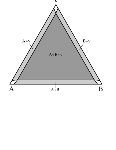
FIG. 1.: Cut through the phase diagram at constant temperature $kT=0.6\epsilon_{AA}$. The interaction energies are $\epsilon_{AA}=\epsilon_{BB}$ and $\epsilon_{AB}=\epsilon_{AA}/2$. White: one phase, light gray: two phase coexistence, dark gray: three phase coexistence.

From the free energy density, we can obtain the phase diagram. We will consider only completely attractive models here, where no order-disorder transitions occur ($\epsilon_{AA}>0$, $\epsilon_{BB}>0$, $\epsilon_{AA}+\epsilon_{BB}-2\epsilon_{AB}>0$). The conditions for phase coexistence are that the chemical potentials and the grand potential, $\Omega=f-\mu^{A}p^{A}-\mu^{B}p^{B}$ be equal in the two (or three) phases. This is equivalent to a “common tangent plane” construction: the free energy density, function of two variables, defines a surface in the space $(p^{A},p^{B},f)$. The (homogeneous) chemical potentials as functions of $p^{A}$ and $p^{B}$ define the orientation of planes tangent to this surface. The condition of equal grand potential implies that the points representing two (or more) phases in equilibrium must lie in the same plane. Thus we can obtain the phase diagram by constructing all the planes that are tangent to the free energy surface in at least two points. Various structures of phase diagrams can be obtained [42]. For attractive interactions, quite generally the free energy surface has three minima for sufficiently low temperatures. Then, there exists exactly one plane which is tangent in three points: we have three-phase coexistence. Besides, there are families of double tangent planes which give the coexistence lines for two-phase coexistence. For $\epsilon_{AA}=\epsilon_{BB}$, our model is equivalent to the Blume-Emery-Griffiths model [43]. We will focus in this paper on the specific example $\epsilon_{AB}=\epsilon_{AA}/2$. As we then have $\epsilon_{AA}=\epsilon_{BB}=\epsilon_{AA}+\epsilon_{BB}-2\epsilon_{AB}$, the phase diagram is completely symmetric with respect to the interchange of any two components and may be calculated using the analogy with the three state Potts model (see appendix). The phase diagram for $kT/\epsilon_{AA}=0.6$ and $z=4$ (two dimensions) is shown in Fig. 1. There is a large region where an A-rich, a B-rich, and a vacancy-rich “vapor” phase coexist. In the regions of two-phase coexistence, the concentration of the third component is very low.

From formula (21) we can immediately deduce that the mobility in the dilute “vapor”-phase, where $p^{A}$ and $p^{B}$ are small, is much larger than in the two dense phases. As we have $\epsilon_{AA}=\epsilon_{BB}>\epsilon_{AB}$, the diffusion of the minority component is always faster than that of the majority component in the dense phases.

III Simulations

The part of the phase diagram which is most appropriate for the description of an alloy is the region of AB-coexistence with low vacancy concentration. All studies of lattice gas dynamics with vacancies we are aware of are limited to this area. We will investigate the behavior of finite “droplets” of such a material immersed in a stable “vapor”, a very natural situation which can arise for instance when droplets of a liquid mixture in coexistence with its vapor are rapidly quenched into an unstable state. Evidently, our model is not adapted to describe diffusion processes in a vapor, where diffusion does not take place via activated jumps to nearest neighbor sites. But the important feature of this “vapor” phase is that diffusion is much faster than inside the “solid”. Moreover, the atomic mobility decreases continuously across the vapor-mixture interface, and hence at the surface the diffusion is faster than inside the bulk. As we shall see, this induces fast surface modes.

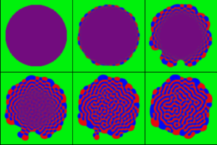
FIG. 2.: Snapshot pictures of the decomposition of a droplet on a $128\times 128$ lattice with periodic boundary conditions. Parameters are: $\epsilon_{AA}=\epsilon_{BB}=1$, $\epsilon_{AB}=0.5$, $kT=0.5$, $p_{\rm sol}^{A}=p_{\rm sol}^{B}=0.46464$, and $p_{\rm vap}^{A}=p_{\rm vap}^{B}=0.03536$. The intensities of red, blue, and green are proportional to $p^{A}$, $p^{B}$, and $p^{v}$, respectively. The pictures are taken at $t=14$, $24400$, $49400$, $74400$, $99400$, and $149200$ $w_{0}^{-1}$.

We integrated the mean-field kinetic equations by an explicit Euler scheme. The time step is limited by the numerical stability of the algorithm. For our inhomogeneous system, the “most dangerous” regions of the simulation domain are those where the diffusion is fastest, thus the vapor phase. For the diffusion equation with a diffusivity $D_{\rm vap}$, the maximum time step is $D_{\rm vap}/2da^{2}$ in $d$ dimensions. For the temperatures and vapor compositions we used, $D_{\rm vap}/a^{2}w_{0}$ is slightly less than unity. We integrated with a maximum time step of $1/4w_{0}$ in 2D and $1/6w_{0}$ in 3D without encountering numerical instabilities. When we started with step functions as initial conditions, the time step had to be chosen much smaller at the beginning and was then slowly increased to the maximum value.

As initial state, we chose “droplets” (i. e. circular domains) or slabs of a mixture with few vacancies (typically some percents) and concentrations $p_{\rm sol}^{A}$ and $p_{\rm sol}^{B}$, immersed in a vapor of concentrations $p_{\rm vap}^{A}$ and $p_{\rm vap}^{B}$. To trigger the phase separation, we added small fluctuations to the initial state. To assure mass conservation, pairs of neighboring sites and a component (A or B) were randomly chosen, and the concentrations at the two sites were shifted by $+A_{0}r$ and $-A_{0}r$, respectively, where $r$ is a random number uniformly distributed between $-1$ and $1$. The noise amplitude $A_{0}$ ranged between $10^{-5}$ and $10^{-2}$. For 2D simulations, we used a lattice of size $128\times 128$ with periodic boundary conditions. All our simulations were carried out on workstations and took from 2 to 20 hours of CPU time. We also simulated two 3D-samples on a $32\times 32\times 64$ lattice; these took up to 100 hours CPU time.

Let us first discuss critical quenches ($p_{\rm sol}^{A}=p_{\rm sol}^{B}$). Snapshot pictures from the time evolution of a droplet are shown in Fig. 2. Phase separation starts at the surface: a fairly regular modulation appears along the mixture-vapor interface. This surface mode triggers phase separation in adjacent regions and propagates into the interior of the sample with a constant velocity, leaving behind a checkerboard-like ordered structure. The domains often coalesce to form stripes.

To see more in detail what happens at the interface, we plot in Fig. 3 several snapshots of the concentration profiles along a line which is normal to the surface at a randomly chosen point. The initial step profile quickly relaxes to a smooth shape and stays nearly stationary, until on a slower time scale B is enriched and A depleted; at other interface points, the opposite happens. An oscillatory concentration profile develops, with an amplitude which has its maximum in the interface and decays into the solid. We will show below that the envelope of this oscillation becomes a decaying exponential away from the surface. The fact that the perturbation decays exponentially with the distance from the surface, but grows exponentially with time, explains the constant propagation velocity of the decomposition front. Note that the concentrations in the vapor vary only very slightly: the vapor is a stable phase, and hence perturbations decay. Because of the fast diffusion in the vapor, the surroundings of the droplet act as a particle reservoir.

           

FIG. 3.: Plots of $p^{A}_{n}$ (a) and $p^{B}_{n}$ (b) along a line normal to a flat interface. From the initial step profile, concentrations rapidly relax to a smooth profile. Then, on a longer time scale, phase separation of A and B occurs, starting from the surface. Times in units of $w_{0}^{-1}$.

As the surface mode develops, the mixture-vapor interface deforms, and fingers of vapor start to grow into the interior of the droplet. This is the result of a Mullins-Sekerka instability [44] with respect to the vacancies. To clarify this point, we show in Fig. 4 snapshots of the vacancy concentration during the decomposition process. At the beginning, the vacancy concentration stays constant and equal to the initial value. Once the decomposition process reaches its nonlinear stage, however, vacancies are expelled from the domains of the new equilibrium phases. These excess vacancies have to diffuse to the surface of the droplet. A finger of vapor protruding into the mixture enhances the concentration gradients around its tip, and hence grows faster than a flat portion of the surface. In addition, the diffusion is faster in the initial mixture than in the phase-separated domains. The growth of the fingers stops when a layer of decomposed material has formed around their entire contour. The diffusion then takes place mainly along the domain boundaries, where the vacancies are enriched. The fingers are smoothed out by the subsequent coarsening process.

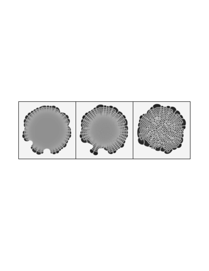
FIG. 4.: Vacancy distribution during the simulation of Fig. 2. Dark areas have low vacancy content. The contrast inside the droplet has been enhanced. Vacancies accumulate in the domain boundaries. The pictures correspond to snapshots number 3,4, and 6 in Fig. 2 ($t=49400$, $74400$, and $149200$ $w_{0}^{-1}$).

The propagation of the surface mode stops when the bulk modes enter the nonlinear regime. The structures in the interior of the sample are the usual bicontinuous patterns of bulk spinodal decomposition at equal volume fractions. Both surface and bulk structures coarsen by the evaporation-condensation mechanism. This process is faster at the surface because of the rapid diffusion through the vapor. At the exterior surface of the droplet, there exist trijunction points where the three phases are in contact. The angles between the interfaces at these points are fixed by the local equilibrium between the three surface tensions of Av, Bv, and AB-interfaces. For our symmetric choice of interaction energies, all angles are $120^{\circ}$ in local equilibrium.

The initial values for the concentrations in our example represent a special choice: the chemical potentials of the two species and the grand potential have the same value in the mixture and in the vapor. There exists exactly one set of concentrations satisfying these conditions at a given temperature. In this special case, there is no net mass flux between vapor and mixture, and the interface is at rest. This choice was mainly made to simplify the stability calculations to be presented below. The existence of a surface mode, however, is not limited to this special case. For other initial conditions (but still $p_{\rm sol}^{A}=p_{\rm sol}^{B}$ and $p_{\rm vap}^{A}=p_{\rm vap}^{B}$), a surface mode develops while the mixture-vapor interface slowly moves.

To obtain more quantitative information about the phase separation process, we repeated our simulation with the same parameters, but this time in a stripe geometry: a slab of mixture along the $y$-direction is immersed in the vapor; we thus have two straight interfaces normal to the $x$ axis. A convenient quantity for the analysis of phase separation processes is the dynamical structure factor. Of particular interest in our case is the difference between bulk and surface behavior. Therefore, we define a one-dimensional structure factor along the interface:

$$S^{\alpha}(k_{y},x,t)=\left|{1\over L_{y}}\sum_{\{j|x_{j}=x\}}p_{j}^{\alpha}e^{ik_{y}y_{j}}\right|^{2},$$ (22)

where $x_{j}$ and $y_{j}$ are the coordinates of lattice site $j$. The sum goes over a lattice plane (in 2D: a line) at a fixed $x$-coordinate, and $k_{y}$ is parallel to the surface. Figure 5 shows plots of this quantity for different times.

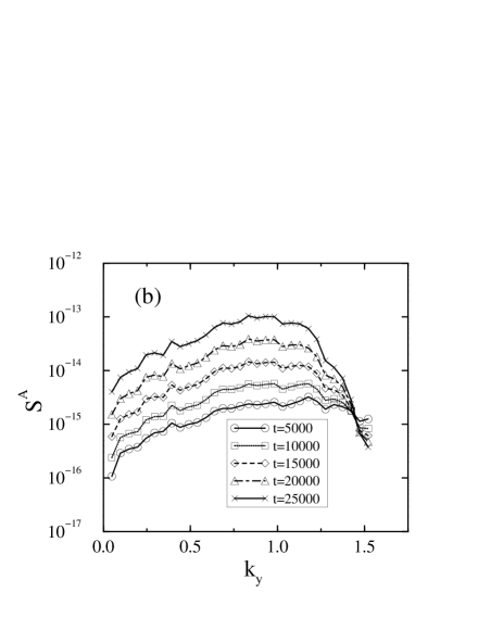
FIG. 5.: Plots of $S^{A}(k_{y},x,t)$ (a) for the first solid layer and (b) in the middle of the slab. The data are averaged over 10 runs with different initial fluctuations (noise amplitude $A_{0}=0.5\times 10^{-5}$).

We observe the characteristic Cahn-Hilliard behavior: in the beginning, linear superposition is valid, and the structure factor for each mode grows exponentially with a growth rate depending on $k_{y}$. In particular, all the structure factor curves intersect in one point, corresponding to the marginally stable mode. At later times, the nonlinear terms in the equations of motion couple the different modes, and the shape of the structure factor curve changes, as can be noted at the last time for the surface layer. The two sets of curves have very different amplitudes, and the maximum is located at $ak_{y}\approx 0.3$ at the surface, and at $ak_{y}\approx 1$ in the bulk. These differences between bulk and surface behavior will be addressed in Sec. 4.

Very different structures appear when the concentration of the mixture is sufficiently off-critical. Fig. 6 shows the evolution of a slab of an AB mixture with a concentration ratio 60:40. The initial concentrations were again chosen to give equal chemical potentials and grand potential in the two bulk phases; note that now $\mu^{A}\neq\mu^{B}$. The minority component rapidly segregates at the surface, triggering a “spinodal wave” normal to the surface. A surface mode with modulations along the interface is still present and leads to a destabilization of the first layer of the minority component, which disintegrates into regularly spaced droplets. These droplets coarsen rapidly. This time, there is no Mullins-Sekerka instability with respect to the vacancies, because the formation of the first decomposed layer rapidly blocks the exchange of vacancies between the interior of the sample and the vapor.

Inside the sample, the surface-induced wave travels until the bulk modes reach their nonlinear regime. There is a competition of droplet and stripe patterns during the subsequent coarsening process. The droplets in the interior of the sample coarsen more rapidly than the stripes at the surface, not surprisingly as the driving force for the evaporation-condensation mechanism of coarsening is the curvature of the domain walls. Ultimately, the stripes start to break up and are “infected” by the droplet pattern.

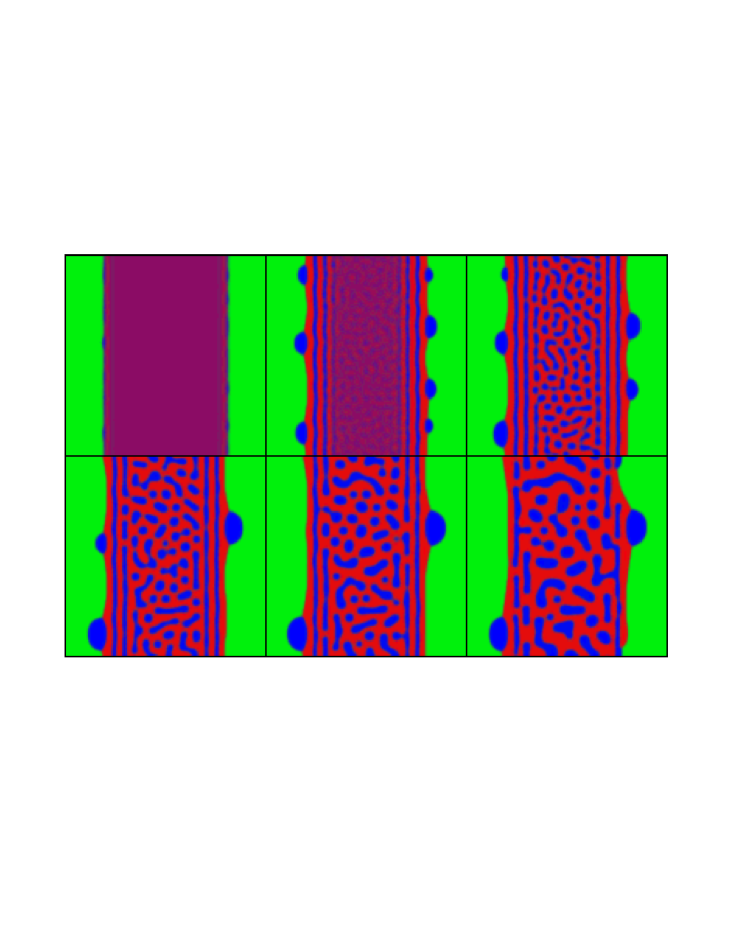
FIG. 6.: Snapshot pictures of a mixture with $p_{\rm sol}^{A}=0.56007$, $p_{\rm sol}^{B}=0.37338$ in a vapor of $p_{\rm vap}^{A}=0.04507$, $p_{\rm vap}^{B}=0.03019$. The other parameters and the colors are as in Fig. 2. $t=10600$, $60700$, $123200$, $248300$, $373400$, and $623500$ $w_{0}^{-1}$.

A simulation for a “droplet” geometry is shown in Fig. 7. The obviously symmetric configuration of the outer domains of B-rich phase is due to the anisotropy of the surface tensions introduced by the lattice [38]. It is interesting to note that this effect is not immediately visible in the critical quenches. The symmetric configuration, however, is only transient: on the last snapshot picture, the smallest of the four outer B domains is about to evaporate. Note also the symmetry in the first and second ring of inner droplets; this pattern is later destroyed by the coarsening of the bulk structures.

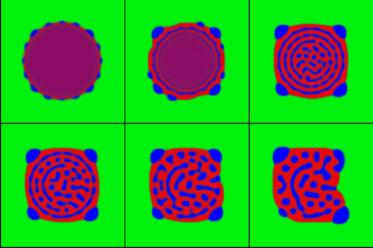
FIG. 7.: Same parameters as the preceding figure, but in circular geometry. The symmetries in the picture are a consequence of the lattice structure. Times: $10600$, $35600$, $123200$, $248300$, $373400$, and $623500$ $w_{0}^{-1}$

Figure 8 shows the evolution of the interface profiles. In contrast to the critical quench, there is no smooth, nearly stationary state at intermediate times. The profile immediately starts to show the onset of oscillations. Also, the evolution is faster: at $t=12000w_{0}^{-1}$, when the separation of A and B is still tiny in Fig. 3, it is already well pronounced in the off-critical case.

           

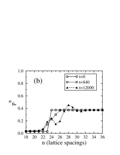
FIG. 8.: Same as Figure 3, but for an off-critical quench. Note the faster evolution. Times in units of $w_{0}^{-1}$.

The difference between the two evolutions can be qualitatively understood by a look on the free energy surface, plotted in Fig. 9. In this figure, the points a, b, and c denote the initial compositions of the critical and off-critical mixtures and the vapor, respectively. In the symmetric case, we can connect the points a and b along a symmetry axis of the free energy density, with zero slope along the A-B-direction. This means that an interface which is situated completely on this line is stationary with respect to a separation of A and B. For the case of an off-critical concentration, we cannot find any such line going from b to c, and an unstable stationary interface does not exist. At the surface of the mixture, chemical potential gradients will always lead to a segregation of one of the components to the surface. Which component is attracted to the surface depends on the choice of concentrations in the vapor phase. Let us mention that this argument is not entirely complete, because it considers only the free energy density, whereas the complete free energy also contains the discrete gradient terms. In our simulations, however, we never observed any unstable stationary interface configuration for off-critical compositions (or asymmetric interaction energies).

The transition from the checkerboard structures to the stripes is gradual. For slightly asymmetric concentrations, the segregation to the surface is slow, and the surface mode has enough time to grow. We observed checkerboard structures up to a concentration ratio of approximately 54:46. For this composition, checkerboard structures and stripes appear simultaneously on different portions of the surface. Similar findings are also valid when we vary the interaction parameters in our model: for $\epsilon_{BB}\neq\epsilon_{AA}$, we have always observed surface-directed spinodal waves; however, a surface mode should appear in this case if for some asymmetric compositions the surface segregation becomes slow.

These findings are consistent with calculations for mixtures near flat substrates using continuous equations of Cahn-Hilliard type: spinodal waves occur when one component is attracted to the substrate [12, 13], whereas surface modes have been found in the case of a substrate which prefers neither of the components of the mixture [14]. Our simple model shows that this general behavior is also valid for free surfaces.

FIG. 9.: Free energy surface, represented by its isoenergy lines, for $kT/\epsilon_{AA}=0.5$. The three minima near the corners are separated by a “hill” in the center.

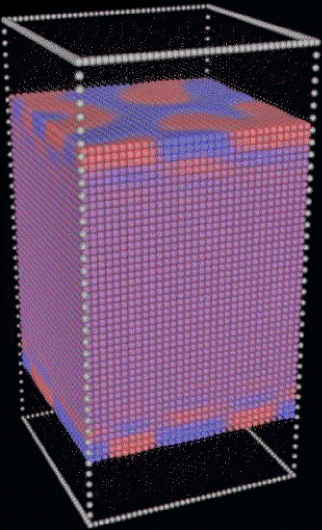
FIG. 10.: 3D sample on a $32\times 32\times 64$ lattice at critical composition (initial concentrations as in Fig. 2, $kT/\epsilon_{AA}=0.75$). The outer white spheres indicate the limits of the simulation box. Periodic boundary conditions are applied in all directions. The size of each sphere inside the box indicates the total concentration ($p^{A}+p^{B}$), the color its composition (red: A, blue: B). Regions of vapor are situated above and below the mixture film; as the concentration of atoms is very low in these regions, the corresponding spheres are tiny. This snapshot was taken at $t=20400w_{0}^{-1}$.

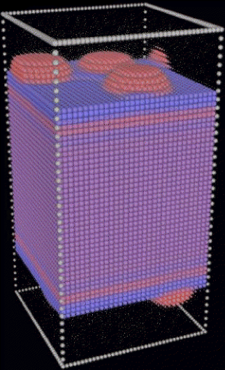
FIG. 11.: 3D sample at off-critical composition. Initial concentrations are as in Fig. 6, $kT/\epsilon_{AA}=0.75$, and $t=20400w_{0}^{-1}$.

In 3D samples we also find fast surface modes, but because the vapor-mixture interface is now two-dimensional, the patterns occurring at the surface for critical quenches are those of 2D bulk spinodal decomposition (Fig. 10). A bicontinuous pattern forms at the surface and propagates into the sample, replicating itself in an oscillatory manner, that is we always find an oscillating concentration profile when we look normal to the surface. In the off-critical case, a spinodal wave occurs as in two dimensions (Fig. 11).

In all the simulations presented so far, the domains of the A- and B-rich phases stick together, because the surface tension of an Av- or Bv-interface is more than the half of the one of an AB-interface. This changes if we lower the interaction energy $\epsilon_{AB}$: for $\epsilon_{AB}=0$, the droplet “explodes”: thin layers of vapor penetrate into the interior of the droplet along the forming AB-interfaces, and the domains of A and B are slowly drifting apart (Fig. 12). This reminds of the decomposition of a binary mixture in the presence of a surfactant. The presence of sharp corners and facets in the domain shapes of the last snapshot indicates that the surface tension anisotropy is quite large.

IV Linear stability analysis

A Bulk

We will now study more in detail the checkerboard structures. To this end, we must calculate the growth rates of bulk and surface modes. We start with the bulk modes. A homogeneous system of overall composition $\bar{p}^{A}$ and $\bar{p}^{B}$ is perturbed by small fluctuations of the occupation probabilities:

$$p_{i}^{\alpha}(t)=\bar{p}^{\alpha}+\delta_{i}^{\alpha}(t)\quad(\alpha=A,B),$$ (23)

with $\delta_{i}^{\alpha}\ll 1$. We linearize the chemical potentials around the average concentrations. Introducing a vector notation with respect to the two species of particles, we obtain starting from Eqs. (15)

$$\left(\begin{array}[]{c}\mu_{i}^{A}\\ \mu_{i}^{B}\end{array}\right)=\left(\begin{array}[]{c}\bar{\mu}^{A}\\ \bar{\mu}^{B}\end{array}\right)-{\bf E}\left(\begin{array}[]{c}{\Delta_{a}}\delta_{i}^{A}\\ {\Delta_{a}}\delta_{i}^{B}\end{array}\right)+{\bf S}\left(\begin{array}[]{c}\delta_{i}^{A}\\ \delta_{i}^{B}\end{array}\right).$$ (24)

Here, $\bar{\mu}^{\alpha}$ are the unperturbed values of the chemical potentials, the matrix ${\bf E}$ of the interaction energies is

$${\bf E}=\left(\begin{array}[]{cc}\epsilon_{AA}&\epsilon_{AB}\\ \epsilon_{AB}&\epsilon_{BB}\end{array}\right),$$ (25)

and $S$ is the matrix of the second derivatives of the free energy density, taken at $\bar{p}^{A}$ and $\bar{p}^{B}$:

$${\bf S}=\left(\begin{array}[]{cc}S_{AA}&S_{AB}\\ S_{AB}&S_{BB}\end{array}\right)\quad{\rm with}\quad S_{\alpha\beta}={\left.{\partial^{2}f\over\partial p^{\alpha}\partial p^{\beta}}\right|}_{\bar{p}^{A},\bar{p}^{B}}.$$ (26)

The variations in the chemical potentials create currents. To obtain these currents to order one in $\delta_{i}^{\alpha}$, we may use the unperturbed values of the mobilities,

$$M_{ij}^{\alpha}=M_{\rm hom}^{\alpha}(\bar{p}^{A},\bar{p}^{B})=\bar{M}^{\alpha}.$$ (27)

The equations of motion become:

$${d\over dt}\left(\begin{array}[]{c}\delta_{i}^{A}\\ \delta_{i}^{B}\end{array}\right)=\left(\begin{array}[]{c}\bar{M}^{A}{\Delta_{a}}\mu_{i}^{A}\\ \bar{M}^{B}{\Delta_{a}}\mu_{i}^{B}\end{array}\right).$$ (28)

As a homogeneous system is translation invariant with respect to the lattice vectors, solutions of the linearized equations are of the form:

$$\left(\begin{array}[]{c}\delta_{j}^{A}\\ \delta_{j}^{B}\end{array}\right)=\left(\begin{array}[]{c}\delta^{A}\\ \delta^{B}\end{array}\right)\exp\left(i\vec{k}\cdot\vec{x}_{j}+\omega(\vec{k})t\right),$$ (29)

where $\vec{x}_{j}$ is the position vector of site $j$ in real space, and $\vec{k}=(k_{x},k_{y})$ is the wave vector of the perturbation. The growth rate $\omega(\vec{k})$ and the coefficients $\delta^{\alpha}$ have to be determined by solving the eigenvalue problem

$$\omega(\vec{k})\left(\begin{array}[]{c}\delta^{A}\\ \delta^{B}\end{array}\right)=A_{\vec{k}}\left(\begin{array}[]{cc}\bar{M}^{A}&0\\ 0&\bar{M}^{B}\end{array}\right)\,\left({\bf S}-A_{\vec{k}}{\bf E}\right)\left(\begin{array}[]{c}\delta^{A}\\ \delta^{B}\end{array}\right).$$ (30)

Here, the terms

$$A_{\vec{k}}=-4\sin^{2}(k_{x}a/2)-4\sin^{2}(k_{y}a/2)$$ (31)

arise from the discrete Laplacians. Eq. (30) is quadratic in $\omega$ and thus gives a stability spectrum

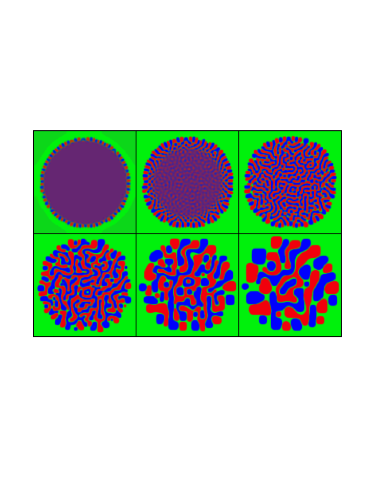
FIG. 12.: Decomposition of a droplet of initial compositions $p_{\rm sol}^{A}=p_{\rm sol}^{B}=0.4276$ in a vapor with $p_{\rm vap}^{A}=p_{\rm vap}^{B}=0.0724$ for $\epsilon_{AA}=\epsilon_{BB}=1,\epsilon_{BB}=0,kT=0.4$. The snapshot times are $t=560$, $1590$, $4130$, $14100$, $48830$, and $149010$ $w_{0}^{-1}$.

with two branches. Each of these branches can be stable ($\omega$ is negative for all wave vectors) or unstable. In the latter case, positive growth rates occur for small values of $|\vec{k}|$. The number of unstable branches is equal to the number of negative eigenvalues of the matrix $\bf S$. This can be easily seen by taking the limit $|\vec{k}|\to 0$ in Eq. (30). The terms proportional to $A_{\vec{k}}^{2}$ can be neglected, and we have

$$\omega(\vec{k})\left(\begin{array}[]{c}\delta^{A}\\ \delta^{B}\end{array}\right)=-{|\vec{k}|}^{2}{\bf S}\left(\begin{array}[]{c}\delta^{A}\\ \delta^{B}\end{array}\right).$$ (32)

The matrix S is related to the curvature of the free energy surface. If both eigenvalues are positive, the surface is locally convex, and the homogeneous state is stable. For two eigenvalues of different sign, the surface has locally the structure of a saddle point, and we have partial instability: only fluctuations in the concave direction in concentration space are amplified. Finally, for two negative eigenvalues, the free energy surface is concave and all perturbations grow. The frontiers between these regions of different stability behavior are given by the spinodal surfaces, defined by the condition

$$\det{\bf S}=0.$$ (33)

This generalizes the concept of a spinodal curve to our three-component system.

FIG. 13.: Cut through the spinodal surfaces along the plane $p^{A}=p^{B}$ (left) and the typical behavior of the dispersion relations $\omega_{+}(\vec{k})$ and $\omega_{-}(\vec{k})$ (right). In region I, the system is stable, in region II it is unstable against separation of particles and vacancies, in region IV against separation of A and B; in region III, it is completely unstable.

For the special case of symmetric interaction energies and equal average concentration, Eq. (30) can be considerably simplified because then we have $\bar{M}^{A}=\bar{M}^{B}=\bar{M}$. In addition, the matrix $\bf L$ defined by

$${\bf L}=A_{\vec{k}}({\bf S}-A_{\vec{k}}{\bf E})$$ (34)

is symmetric. We obtain immediately

$$\omega_{\pm}(\vec{k})=\bar{M}(L_{AA}\pm L_{AB}),$$ (35)

and the associated eigenvectors are

$$\left(\begin{array}[]{c}\delta^{A}\\ \delta^{B}\end{array}\right)=\left(\begin{array}[]{c}1\\ \pm 1\end{array}\right).$$ (36)

This last result shows that of the two branches of the dispersion relation, the first describes the separation into a dense AB mixture and a dilute vapor, whereas the second gives a separation between A and B, leaving the local vacancy concentration unchanged. Fig. 13 shows a cut through the spinodal surfaces along the axis $\bar{p}^{A}=\bar{p}^{B}$. We also indicate the regions of different stability behaviors, and show the typical shapes of $\omega_{+}(\vec{k})$ and $\omega_{-}(\vec{k})$ in these regions. The interior of our samples is in the region where only the mode separating A and B is unstable: the local vacancy concentration stays unchanged in the linear stage. Other modes of decomposition in a homogeneous ternary system have been studied by Chen [35].

The anisotropy due to the lattice structure enters in the above formulae by the factor $A_{\vec{k}}$. For the long wavelength perturbations considered here ($a|\vec{k}|<1$), the relative variations of $A_{\vec{k}}$ with orientation are of the order of a percent. We will therefore neglect this dependence and use a wave vector along one of the lattice directions for comparisons to numerical results. For the example of the simulation shown in Fig. 2, i.e. with $kT/\epsilon_{AA}=0.5$ and $\bar{p}^{A}=\bar{p}^{B}=0.46464$, we found a maximum bulk growth rate of $\omega_{b}=1.06\times 10^{-4}w_{0}$ at a wave number $k_{b}=1.003/a$.

B Surface

We must now analyze the stability spectrum at the surface. This is more difficult than in the bulk because the initial state is now heterogeneous. To simplify the problem, we will treat the case of a flat interface which is normal to one of the lattice directions, say $x$. Then, in the initial state all lattice sites in a layer at a given $x$ coordinate have the same concentrations. In what follows, we will replace the site indices “$i$” used so far by a pair of indices “$n,j$”, where $n$ numbers the layer, and $j$ numbers the sites in the $y$ direction. We use the same values of the concentrations in the bulk phases as for our simulations. As the chemical potentials are equal in the two phases, the initial interface state can be obtained by fixing the chemical potentials to their appropriate values and numerically solving the one-dimensional version of the finite difference equations Eq. (15) for the concentrations in the $n$th layer $\bar{p}^{\alpha}_{n}$.

Whereas the translation invariance is broken along the $x$-axis, it is preserved along $y$, and hence we can still use a Fourier representation. We write the perturbed state as

$$p^{\alpha}_{n,j}(t)=\bar{p}^{\alpha}_{n}+\delta_{n,j}^{\alpha}(t),$$ (37)

$$\delta_{n,j}^{\alpha}(t)=\delta_{n}^{\alpha}\exp\left(ik_{y}ja+\omega(k_{y})t\right),$$ (38)

with two unknown coefficients $\delta^{A}_{n}$ and $\delta^{B}_{n}$ per layer. We start with the linearization of the chemical potentials. The discrete Laplacians appearing in Eq. (15) give contributions of the form

$${\Delta_{a}}\delta_{n,j}^{\alpha} = \delta_{n+1,j}^{\alpha}+\delta_{n-1,j}^{\alpha}+\delta_{n,j+1}^{\alpha}+\delta_{n,j-1}^{\alpha}-4\delta_{n,j}^{\alpha}$$ (39)

$$= \left[\delta^{\alpha}_{n-1}+\delta^{\alpha}_{n+1}+\left(A_{\vec{k}}-2\right)\delta_{n}^{\alpha}\right]\,\exp\left(ik_{y}ja+\omega(k_{y})t\right).$$ (40)

Denoting by $\bar{\mu}^{\alpha}$ the (constant) values of the unperturbed chemical potential, and by ${\bf S}(n)$ the matrix of the second derivatives, taken at $\bar{p}_{n}^{A}$ and $\bar{p}_{n}^{B}$, we find

$$\left(\begin{array}[]{c}\mu^{A}_{n,j}-\bar{\mu}^{A}\\ \mu^{B}_{n,j}-\bar{\mu}^{B}\end{array}\right)=\left({\bf S}(n)-(A_{\vec{k}}-2){\bf E}\right)\left(\begin{array}[]{c}\delta^{A}_{n,j}\\ \delta^{B}_{n,j}\end{array}\right)-{\bf E}\left(\begin{array}[]{c}\delta^{A}_{n-1,j}\\ \delta^{B}_{n-1,j}\end{array}\right)-{\bf E}\left(\begin{array}[]{c}\delta^{A}_{n+1,j}\\ \delta^{B}_{n-1,j}\end{array}\right).$$ (41)

The next step is the linearization of the equations of motion. As in the homogeneous case, the mobilities can be taken in the unperturbed initial state. But because the concentrations vary through the interface, we cannot use the expression for the homogeneous system. The appropriate expressions can be obtained from Eq. (14) by taking the limit $\mu_{j}\to\mu_{i}$ with $p_{j}\neq p_{i}$:

$$\bar{M}_{mn}^{\alpha}=w_{0}{(1-\bar{p}_{m}^{A}-\bar{p}_{m}^{B})(1-\bar{p}_{n}^{A}-\bar{p}_{n}^{B})\over kT}\exp\left(\bar{\mu}^{\alpha}\over kT\right)$$ (42)

(the two indices of $\bar{M}_{nm}$ are two layer indices). The linearized equation of motion becomes

$${d\over dt}\delta_{n,j}^{\alpha}=\bar{M}^{\alpha}_{nn}\left(\mu^{\alpha}_{n,j+1}-2\mu^{\alpha}_{n,j}+\mu^{\alpha}_{n,j-1}\right)+\bar{M}^{\alpha}_{nn+1}\left(\mu^{\alpha}_{n+1,j}-\mu^{\alpha}_{n,j}\right)+\bar{M}^{\alpha}_{nn-1}\left(\mu^{\alpha}_{n-1,j}-\mu^{\alpha}_{n,j}\right).$$ (43)

Inserting Eqs. (41) and (38), one obtains an eigenvalue problem for $\omega$, the eigenvectors given by the set of unknown coefficients $\delta_{n}^{\alpha}$. This means that the matrix to diagonalize is of size $2L\times 2L$, where $L$ is the number of layers in the $x$ direction, and that the corresponding dispersion relation has $2L$ branches. This is a standard linear algebra problem and can be solved numerically.

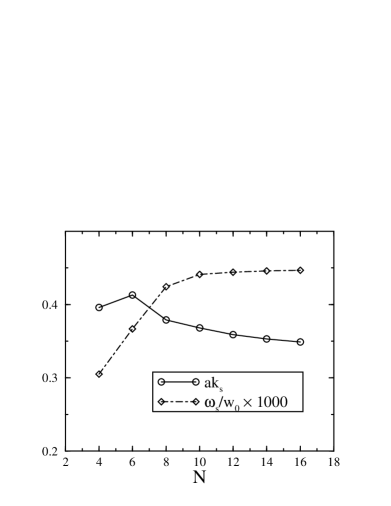
FIG. 14.: Maximum growth rate $\omega_{s}$ and corresponding wave vector $k_{s}$ for the vapor-mixture interface with initial conditions as in Fig. 2 as a function of the number $N$ of layers around the interface included in the eigenvalue problem.

In the initial stage of the development, the surface mode is localized in a small number of layers around the surface. Hence we can simplify the problem by considering a small “solution region” around the interface. We assume perturbations outside a narrow region of $N$ layers centered around the interface to be zero. We diagonalized the resulting $2N\times 2N$ matrix numerically and obtained the maximum growth rate, $\omega_{s}$, and the corresponding wave vector $k_{s}$. As shown in Fig. 14, these quantities become independent of $N$ if a sufficient number of layers is included [45].

FIG. 15.: Comparison of theoretical prediction (line) and simulation results (circles) for the stability spectrum of the vapor-mixture interface with the same parameters as in Fig. 2. The theoretical curve is calculated with $N=16$, the growth rates in the simulation were extracted from the data in Fig. 5. The scatter in the simulation data is due to the finite number of different runs.

To compare the results of this stability analysis to the simulations, we extracted the stability spectrum of the surface from the structure factor data of Fig. 5. For an exponentially growing Fourier mode, we have $S(t)\propto\exp(2\omega t)$, and the growth rate can be obtained as $\omega=\ln(S(t_{2})/S(t_{1}))/2(t_{2}-t_{1})$. Fig. 15 shows that the agreement with the theoretical prediction is excellent, except for very small wave numbers. This discrepancy can be explained by the fact that for large wavelengths, more layers have to be included, as the diffusion field in the vapor will be appreciably modified up to a distance from the interface which is comparable to the wavelength. In conclusion, the maximum growth rate and the corresponding wave vector can be accurately predicted by a calculation involving only a small number of layers.

For the example of Fig. 2, we find a maximum growth rate of $\omega_{s}=4.47\times 10^{-4}w_{0}$ at a wave number $k_{s}=0.349/a$. This surface mode grows more than four times faster than the fastest bulk mode, and at a wavelength about three times larger than the wavelength of the typical bulk pattern. We verified indeed in our simulations that the “incubation time”, i. e. the time after which the growing perturbations become visible in a given visualization, was about four times larger in the bulk than at the surface.

TABLE I.: Characteristic quantities for bulk and surface modes in two dimensions for different temperatures

$kT/\epsilon_{AA}$	0.4	0.5	0.6	0.7
$p_{\rm vap}^{A}$,$p_{\rm vap}^{B}$	0.0141	0.0354	0.0724	0.1412
$p_{\rm sol}^{A}$,$p_{\rm sol}^{B}$	0.4859	0.4646	0.4276	0.3588
$\omega_{b}/w_{0}\times 1000$	0.016	0.106	0.255	0.008
$\omega_{s}/w_{0}\times 1000$	0.383	0.447	0.342	0.003
$\omega_{s}/\omega_{b}$	23.9	4.21	1.34	0.36
$ak_{b}$	1.147	1.003	0.793	0.222
$ak_{s}$	0.312	0.349	0.421	0.132
$k_{b}/k_{s}$	3.68	2.87	1.88	1.68

TABLE II.: Same as table I, but in three dimensions.

$kT/\epsilon_{AA}$	0.6	0.75	0.9	1.05
$p_{\rm vap}^{A}$,$p_{\rm vap}^{B}$	0.0141	0.0354	0.0724	0.1412
$p_{\rm sol}^{A}$,$p_{\rm sol}^{B}$	0.4859	0.4646	0.4276	0.3588
$\omega_{b}/w_{0}\times 1000$	0.024	0.159	0.383	0.012
$\omega_{s}/w_{0}\times 1000$	0.976	0.773	0.528	0.007
$\omega_{s}/\omega_{b}$	40.7	4.86	1.37	0.61
$ak_{b}$	1.453	1.259	0.986	0.272
$ak_{s}$	0.414	0.410	0.505	0.204
$k_{b}/k_{s}$	3.51	3.07	1.92	1.33

Having verified that our method gives accurate results, we can apply it to study the behavior of bulk and surface modes for different temperatures. The results are given in Table I. All calculation were performed with $N=16$, except for the highest temperature where $N=32$ was used. The bulk growth rate has a maximum around $kT/\epsilon_{AA}=0.6$ and decreases as the temperature is lowered, because the activated dynamics lead to small values of the mobility for low temperatures. On the other hand, for the highest temperature the system is near a spinodal surface, and the driving force for phase separation is small, leading also to a lower growth rate. The surface growth rate follows the same trends. At the highest temperature considered, $\omega_{s}$ is lower than $\omega_{b}$, which means that a proper surface mode does not exist any more. The ratio $\omega_{s}/\omega_{b}$ increases monotonically as the temperature is lowered. It should be noted that the mean-field approximation becomes increasingly inaccurate for low temperatures. Also, the interfaces become very sharp, which leads to strong lattice effects.

It is also straightforward to repeat these calculations for three dimensions. In fact, the phase diagram stays the same if we scale the temperature by a factor of $1.5$. On the other hand, the interface shapes and the growth rates are different, because the balance between the discrete Laplacians and the local terms is altered in Eqs. (15) for the chemical potentials. In the stability calculations, the magnitude of the stability matrix $\bf S$ is modified whereas the terms arising from the Laplacians stay the same. The final results for the growth rates and wave vectors, shown in Table II, are similar to the two-dimensional case.

C Propagation of the surface patterns

The surface mode propagates into the interior of the sample, enforcing its characteristic wavelength in the direction parallel to the surface. This behavior can be understood by considering the solution of the eigenvalue equation away from the interface. Even if the surface modes are localized at the vapor-mixture interface, they are eigenmodes of the whole system and grow everywhere with the same growth rate $\omega_{s}$. But away from the interface, the initial state becomes homogeneous, and we can use Eq. (35), derived for the bulk, if we allow for a decay of the amplitude in the direction normal to the interface by introducing a complex wave number $k_{x}$. As the growth rate and the $y$-component of the wave vector are already known from the analysis of the surface instability, $k_{x}$ is the only remaining unknown. The relevant dispersion relation is $\omega_{-}(\vec{k})$, and we obtain the equation

$$A_{\vec{k}}^{2}\left(\epsilon_{AA}-\epsilon_{AB}\right)-A_{\vec{k}}\left(S_{AA}-S_{AB}\right)+{\omega_{s}\over\bar{M}}=0.$$ (44)

This equation can either be solved numerically using the exact expression for $A_{\vec{k}}$ or analytically with the approximation $A_{\vec{k}}\approx-k_{x}^{2}-k_{y}^{2}$. The latter method leads to a biquadratic equation for $k_{x}$. In both cases, there are four solutions of the form

$$k_{x}=\pm k^{\prime}\pm ik^{\prime\prime}$$ (45)

with $k^{\prime}$ and $k^{\prime\prime}$ real and positive. The two solutions with negative imaginary part diverge in the bulk and have to be discarded. The other two solutions lead to modes proportional to $\exp(\pm ik^{\prime}x+\omega_{s}t-k^{\prime\prime}x)$, that is modes with an oscillatory concentration profile and an envelope which decays exponentially with the distance from the surface, but grows exponentially in time. One can define a propagation velocity of the decomposition front by the phase velocity of the envelope,

$$v={\omega_{s}\over k^{\prime\prime}}.$$ (46)

We compared the values for the wavelength normal to the surface, $\lambda_{x}=2\pi/k^{\prime}$, and the propagation velocity obtained by this method to our simulations and found good agreement [18].

The competition between surface and bulk modes leads to the interesting consequence that the thickness of the layer near the surface where the surface-directed patterns prevail depends on the strength of the initial fluctuations. This can be seen as follows. For an exponentially growing mode with initial amplitude $\delta_{0}$, the time to reach a threshold amplitude $\delta_{nl}$ where nonlinear couplings between different modes become important is

$$\tau\sim{1\over\omega}\ln{\delta_{nl}\over\delta_{0}}.$$ (47)

Now, a surface mode “propagates” into the sample approximately between the time $\tau_{s}$ when it is well developed at the surface, and the time $\tau_{b}$ when the bulk modes reach the nonlinear stage. The distance $d$ the front propagates is therefore given by

$$d\sim v(\tau_{b}-\tau_{s})={1\over k^{\prime\prime}}\left({\omega_{s}\over\omega_{b}}-1\right)\ln{\delta_{nl}\over\delta_{0}}.$$ (48)

The thickness of the surface structures depends logarithmically on the strength of the initial noise. This reasoning applies both to the symmetrical checkerboard structures and the surface-directed spinodal waves and was confirmed by our simulations.

V Conclusions

We have developed mean field kinetic equations to describe the dynamics of a lattice gas model of a binary alloy with vacancies (ABv model) in which diffusion takes place by the vacancy mechanism only. Despite the simplicity of the model, we observe a rich variety of phase separation patterns at free surfaces between an unstable mixture and a stable vapor. The most spectacular effect is a fast surface mode. It creates ordered patterns at the surface with a length scale which is clearly distinct from the characteristic scale of the bulk patterns. This mode appears in a small range of parameters around a symmetric point where the mixture-vapor interface is “neutral”, that is none of the components of the mixture segregates to the surface. On the other hand, if such segregation occurs and is rapid enough, the surface mode is suppressed, and instead surface-directed spinodal waves are observed which create a striped pattern along the surface. Both patterns, once they have formed at the surface, propagate into the sample over a distance which is related to the difference in surface and bulk growth rates and the strength of the initial fluctuations.

Our approach starts from a minimal model with very few assumptions. Therefore, it cannot be used to model a particular experimental situation. But it allows to identify some basic ingredients necessary for the formation of such surface structures in a fairly well-defined setting, and we can draw some conclusions which should be generally valid.

The existence of the fast surface mode is related to the fact that in our model the surface atoms are more mobile than in the bulk, an assumption which seems reasonable for many interfaces between a dense and a dilute phase. The characteristic growth rates of the surface modes can be calculated by a linear stability analysis starting from the initial interface profile. We have shown that accurate results can be obtained by solving the resulting eigenvalue problem in a small domain around the interface. The characteristics of the propagation of the decomposition front can be obtained by connecting the solution of the surface problem to the bulk solution. This method could be applied as well to continuum models of Ginzburg-Landau type by using an appropriate discretization.

Which type of surface structure occurs is related to the time scales for segregation and surface phase separation. If the segregation is slow, surface spinodal decomposition is dominant, otherwise spinodal waves are observed. As in a realistic system, the interactions between different species are always different, spinodal waves are the more generic pattern. The surface mode should show up, however, in a small range of initial compositions if the interactions are not too different. More work is needed to clarify this point.

A very interesting point is that the thickness of the layer of surface patterns depends on the initial fluctuation strength. This is not the case in bulk spinodal decomposition, where a rescaling of the initial fluctuations amounts simply to a shift in time. The arguments leading to Eq. (48) are fairly general and should apply to all systems where a fast surface mode is in competition with a slow bulk mode. In rapid quench experiments, the initial fluctuation spectrum is mainly determined by the temperature before the quench. Therefore, the thickness of the surface layer may depend on the initial temperature. In view of the logarithmic dependence of $d$ on the noise strength, this effect might be difficult to observe; however, if the initial state of the system is close to a critical point, the fluctuation amplitude is a rapidly varying function of temperature.

Surface effects in spinodal decomposition have been studied recently in polymers [6, 7, 8, 9, 10, 11]. Evidently, our equations cannot be applied to polymers. But from our results it is simple to construct a Ginzburg-Landau theory in which surface modes occur: it is sufficient to introduce a mobility function which explicitly depends on the density and which enhances diffusion on the surface.

It would be interesting to compare our findings to Monte Carlo simulations which naturally contain the fluctuations. It has been shown, however, that short-range lattice gas models do not exhibit linearly superposed, exponentially growing modes in the early stages of the phase separation. This can be attributed to the fact that the initial noise is too strong for a linearization of the equations of motion to be valid [46]. On the other hand, for models with longer range interactions the Cahn-Hilliard behavior is restored [47], and we would expect surface modes in such models even with stochastic dynamics.

In summary, our approach allows to explore the rich dynamics of the ABv model and to relate the structures that form spontaneously during phase separation to the parameters of the microscopic model. Here, we have only explored a small part of the possible behaviors in this model, because we have limited ourselves to attractive interactions. There are other interesting questions which could be addressed in the framework of this model and using mean field kinetic equations, for example the influence of the vacancy distribution on the coarsening behavior, or the interplay between phase separation, short range ordering and vacancy distribution.

Phase diagram

Let us first show that the Hamiltonian of the ABv-model can be derived from a general ternary Hamiltonian. We assume that the sites of the lattice can now be occupied by three different sorts of atoms, $A$, $B$, or $C$. In terms of the occupation numbers $n_{i}^{A}$, $n_{i}^{B}$, and $n_{i}^{C}$, the energy of a configuration is given by

$$H=-\sum_{\alpha,\beta}\sum_{\langle i,j\rangle}\epsilon^{\prime}_{\alpha\beta}n_{i}^{\alpha}n_{j}^{\beta}-\sum_{\alpha}\sum_{i=1}^{N}{\mu^{\prime}}_{0}^{\alpha}n_{i}^{\alpha}.$$ (49)

The interaction energies in the ternary system are primed to distinguish them from the $\epsilon$’s in Eq. (1). Here, the ${\mu^{\prime}}_{0}^{\alpha}$ are external chemical potentials, equivalent in the spin language to “generalized magnetic fields” acting only on one possible spin state. Using the constraint of single occupancy, $n_{i}^{A}+n_{i}^{B}+n_{i}^{C}=1\,\forall i$, we can eliminate the occupation numbers of one species, say $C$, and we obtain

$$H=-\sum_{\langle i,j\rangle}\left[\epsilon_{AA}n_{i}^{A}n_{j}^{A}+\epsilon_{BB}n_{i}^{B}n_{j}^{B}+\epsilon_{AB}(n_{i}^{A}n_{j}^{B}+n_{i}^{B}n_{j}^{A})\right]-\sum_{i=1}^{N}\left(\mu^{A}_{0}n_{i}^{A}+\mu^{B}_{0}n_{i}^{B}\right),$$ (50)

where the effective interaction energies and chemical potentials appearing in this last equation are

$$\epsilon_{AA} = \epsilon_{AA}^{\prime}+\epsilon_{CC}^{\prime}-2\epsilon_{AC}^{\prime},$$ (51)

$$\epsilon_{BB} = \epsilon_{BB}^{\prime}+\epsilon_{CC}^{\prime}-2\epsilon_{BC}^{\prime},$$ (52)

$$\epsilon_{AB} = \epsilon_{AB}^{\prime}+\epsilon_{CC}^{\prime}-\epsilon_{AC}^{\prime}-\epsilon_{BC}^{\prime},$$ (53)

$$\mu^{A}_{0} = {\mu^{\prime}}^{A}_{0}-{\mu^{\prime}}^{C}_{0}-z\epsilon_{CC}^{\prime}+z\epsilon_{AC}^{\prime}\quad{\rm and}$$ (54)

$$\mu^{B}_{0} = {\mu^{\prime}}^{B}_{0}-{\mu^{\prime}}^{C}_{0}-z\epsilon_{CC}^{\prime}+z\epsilon_{BC}^{\prime}.$$ (55)

When the total number of particles of each species is conserved, the chemical potential terms in Eq. (50) are constants. Then, we are back to the Hamiltonian Eq. (1).

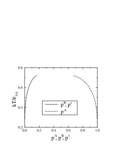
FIG. 16.: Phase diagram of the completely symmetric ABv-model. We show the equilibrium concentrations in the $\alpha$ (A-rich) phase for three-phase coexistence. The concentrations of the other equilibrium phases can be obtained by symmetry. The representative points of the three phases in equilibrium give the central triangle in the diagram in Fig. 1.

Let us now consider the three state Potts model, with ternary interaction energies $\epsilon_{AA}^{\prime}=\epsilon_{BB}^{\prime}=\epsilon_{CC}^{\prime}=1$ and $\epsilon_{\alpha\beta}^{\prime}=0$ for $\alpha\neq\beta$. This gives the effective interactions $\epsilon_{AA}=\epsilon_{BB}=2,\epsilon_{AB}=1$; by changing the temperature scale, we obtain the values $\epsilon_{AA}=\epsilon_{BB}=1,\epsilon_{AB}=0.5$ used in the present paper. Furthermore, from the symmetry of the Potts model it is obvious that three phase coexistence is possible below the critical temperature at zero magnetic fields. This is equivalent, in the ABv model, to

$$\mu^{A}=-z\epsilon_{AA}p^{A}-z\epsilon_{AB}p^{B}+kT{p^{A}\over 1-p^{A}-p^{B}}=-z\epsilon_{AA}/2$$ (56)

and an equivalent equation for $\mu^{B}$. These equations have to be solved numerically to obtain the equilibrium concentrations. The result for the A-rich phase is shown in Fig. 16. The coexistence of A-rich, B-rich, and “vapor”-phases terminates at a quadruple point: a fourth minimum in the free energy surface, located at the symmetric point $p^{A}=p^{B}=p^{v}=1/3$, develops, and at $kT=1/(2\ln 2)\approx 0.721$ the four minima are exactly at the same level. Above this temperature, there is a narrow temperature range above which the four minima persist, but now the fourth minimum is lowest, and we have three different regions of three-phase coexistence (not shown in the figure). Above $kT=0.75$, only the “symmetric” minimum remains.

REFERENCES

- [1] J. W. Cahn and J. E. Hilliard, J. Chem. Phys. 28, 258 (1958).
- [2] J. W. Cahn, Trans. Metall. Soc. AIME 242, 166 (1968).
- [3] J. D. Gunton, M. San Miguel and P. S. Sahni, in Phase Tansitions and Critical Phenomena, Vol. 8, C. Domb and J. L. Lebowitz eds., Academic Press, London (1983)
- [4] K. Binder, in Materials Science and Technology, Vol. 5: Phase Transformations in Materials, edited by P. Haasen, VCH, Weinheim (1991)
- [5] A. J. Bray, Adv. Phys. 43, 357 (1994)
- [6] R. A. L. Jones, L. J. Norton, E. J. Kramer, F. S. Bates and P. Wiltzius, Phys. Rev. Lett. 66, 1326 (1991)
- [7] P. Wiltzius and A. Cumming, Phys. Rev. Lett. 66, 3000 (1991)
- [8] A. Cumming, P. Wiltzius, F. S. Bates and J. H. Rosedale, Phys. Rev. A 45, 885 (1992)
- [9] F. Bruder and R. Brenn, Phys. Rev. Lett. 69, 624 (1992)
- [10] B. Q. Shi, C. Harrison and A. Cumming, Phys. Rev. Lett. 70, 206 (1993)
- [11] C. Harrison, W. Rippard and A. Cumming, Phys. Rev. E 52, 723 (1995)
- [12] S. Puri and K. Binder, Phys. Rev. E 49, 5359 (1994)
- [13] H. L. Frisch, P. Nielaba and K. Binder, Phys. Rev. E 52, 2848 (1995)
- [14] H.-P. Fischer, P. Maass and W. Dieterich, Phys. Rev. Lett. 79, 893 (1997); Europhys. Lett. 42, 49 (1998)
- [15] C. Sagui, A. M. Somoza, C. Roland and R. C. Desai, J. Phys. A: Math. Gen. 26, L1163 (1993)
- [16] C. Geng et L.-Q. Chen, Surf. Sci. 355, 229 (1996)
- [17] P. Keblinski, S. K. Kumar, A. Maritan, J. Koplik and J. R. Banavar, Phys. Rev. Lett. 76, 1106 (1996)
- [18] M. Plapp and J.-F. Gouyet, Phys. Rev. Lett. 78, 4970 (1997)
- [19] K. Kawasaki, in Phase Transitions and Critical Phenomena, Vol. 2, edited by C. Domb et M. S. Green, Academic Press, London (1972)
- [20] M. Rao, M. H. Kalos, J. L. Lebowitz and J. Marro, Phys. Rev. B 13, 4328 (1976)
- [21] J. L. Lebowitz, J. Marro and M. H. Kalos, Acta Metall. 30, 297 (1982)
- [22] D. A. Huse, Phys. Rev. B 34, 7845 (1986)
- [23] J. G. Amar, F. E. Sullivan and R. D. Mountain, Phys. Rev. B 37, 196 (1988)
- [24] G. E. Murch, in Ref. [4]
- [25] K. Yaldram and K. Binder, Acta Metall. 39, 707 (1990); J. Stat. Phys. 62, 161 (1991); Z. Phys. B 82, 405 (1991)
- [26] P. Fratzl and O. Penrose, Phys. Rev. B 50, 3477 (1994); ibid. 53, 2890 (1996); ibid. 55, 6101 (1997)
- [27] C. Frontera, E. Vives and A. Planes, Phys. Rev. B 48, 9321 (1993); C. Frontera, E. Vives, T. Castán and A. Planes, Phys. Rev. B 53, 2886 (1996)
- [28] F. Soisson, A. Barbu and G. Martin, Acta Mater. 44, 3789 (1996)
- [29] A. G. Khatchaturyan, Sov. Phys. Solid State 9, 2040 (1968)
- [30] O. Penrose, J. Stat. Phys. 63, 975 (1990)
- [31] G. Martin, Phys. Rev. B 41, 2279 (1990)
- [32] J.-F. Gouyet, Europhys. Lett. 21, 335 (1993)
- [33] L.-Q. Chen and J. A. Simmons, Acta Metall. Mater. 42, 2943 (1994)
- [34] V. G. Vaks, S. V. Beiden and V. Y. Dobretsov, JETP Lett. 61, 68 (1995)
- [35] L.-Q. Chen, Acta Metall. Mater. 42, 3503 (1994)
- [36] J.-F. Gouyet, Phys. Rev. E 51, 1695 (1995)
- [37] V. Y. Dobretsov, G. Martin, F. Soisson, and V. G. Vaks, Europhys. Lett. 31, 417 (1995); V. Y. Dobretsov, V. G. Vaks, and G. Martin, Phys. Rev. E 53, 5101 (1996)
- [38] M. Plapp and J.-F. Gouyet, Phys. Rev. E 55, 45 (1997); ibid. 55, 5321 (1997)
- [39] L.-Q. Chen, Mat. Res. Soc. Symp. Proc. 319, 375 (1994); C. Geng and L.-Q. Chen, Scripta Metall. Mater. 11, 1507 (1994)
- [40] S. Puri, Phys. Rev. E 55, 1752 (1997); S. Puri and R. Sharma, Phys. Rev. E 57, 1873 (1998)
- [41] R. Kikuchi, Prog. Theor. Phys. Suppl. 35, 1 (1966)
- [42] M. Plapp, PhD thesis, Université Paris XI, Orsay (1997)
- [43] M. Blume, V. J. Emery and R. B. Griffiths, Phys. Rev. A 4, 1071 (1971)
- [44] W. W. Mullins and R. F. Sekerka, J. Appl. Phys. 3, 444 (1964)
- [45] Note that in Ref. [18], we have used no-flux boundary conditions at the limits of the solution region, and obtained quite precise values already with four layers. This method being more cumbersome to implement, we did not carry out a more systematic study.
- [46] K. Binder, Phys. Rev. A 29, 341 (1984)
- [47] M. Laradji, M. Grant, M. J. Zuckermann, and W. Klein, Phys. Rev. B 41, 4646 (1990)