Voronoi-Delaunay analysis of normal modes in a simple model glass.

Abstract

We combine a conventional harmonic analysis of vibrations in a one-atomic model glass of soft spheres with a Voronoi-Delaunay geometrical analysis of the structure. “Structure potentials” (tetragonality, sphericity or perfectness) are introduced to describe the shape of the local atomic configurations (Delaunay simplices) as function of the atomic coordinates. Apart from the highest and lowest frequencies the amplitude weighted “structure potential” varies only little with frequency. The movement of atoms in soft modes causes transitions between different “perfect” realizations of local structure. As for the potential energy a dynamic matrix can be defined for the “structure potential”. Its expectation value with respect to the vibrational modes increases nearly linearly with frequency and shows a clear indication of the boson peak. The structure eigenvectors of this dynamical matrix are strongly correlated to the vibrational ones. Four subgroups of modes can be distinguished.

I Introduction

The thermodynamic properties of glasses at low temperatures differ from those of the corresponding crystals [1]. At low temperatures the specific heat is strongly enhanced compared to the Debye contribution stemming from the sound waves. The excitations underlying this enhancement have been shown to be two-level systems below $T\approx 1$ K and nearly harmonic vibrations above. The vibrational density of state, $Z(\nu)$, plotted as $Z(\nu)/\nu^{2}$ has a maximum, typically near 1 THz, the boson peak.

This low temperature / low frequency behavior can be described by the soft potential model. [2, 3] In this model one assumes that one common type of structural unit is responsible for the excess excitations. One introduces an effective potential describing the motion of this unit. Depending on the parameters this potential is a single well or a double well. In the first case it describes a low frequency localized vibration and in the second tunneling through the barrier (two level systems) or relaxation over the barrier. For low energies one can give a general form for the distribution of the parameters describing the effective potentials. Fitting this model to the experimental data, one finds that 20–100 atoms or molecular units move collectively in the tunneling and in localized vibrations.[4, 5] It should be emphasized that the concept of low frequency localized vibrations is an idealization. These modes will always interact with the sound waves of similar frequency and, therefore, also among each other. This delocalises the modes and they are only quasi-local or resonant. Due to level repulsion, for sufficiently high densities of these modes, the interaction will change their density of states from $Z(\nu)\propto\nu^{4}$ to $Z(\nu)\propto\nu$ thus creating the boson peak.[6] Such a model does, however, not say anything about the physical nature of the localized modes or their origin in different types of glass.

The problem of local dynamics in the amorphous state is closely connected with the problem of the so-called medium-range order in glasses [7, 8]. Recently it has been shown [9, 10] that a computer model of amorphous argon has a heterogeneous structure containing regions of more “perfect” or “imperfect” atomic arrangements on a nanometer scale. In the regions of perfect structure the elementary packings of four neighboring atoms (the Delaunay simplices) are close to either regular tetrahedra or quart-octahedra [9], i.e. quarters of regular octahedra. In the regions of imperfect structure the local configurations of the neighboring atoms differ markedly from these ideal shapes. A partial spectrum of the vibrational states of the atoms in the regions of more “imperfect” structure displays an excess for low-frequency modes.[10]

Quasi-localized low-frequency vibrations have been observed in computer simulations of the soft sphere glass (SSG)[11] and of numerous other materials, such as e.g. SiO₂ [12], Se [13] in Ni-Zr [14] and Pd-Si [15], in amorphous ice [16] and in amorphous and quasi-crystalline Al-Zn-Mg [17]. It was shown that these modes are centered at atoms whose structural surrounding differs substantially from the average. It has been established that the directions of the eigenvectors of soft vibrations strongly correlate with those of the relaxation jumps at low temperatures. [18, 19]

One hypothesis on the origin of the soft mode is that the most active atoms oscillate between neighboring minima of the potential energy formed by a cage of surrounding atoms. [20] These minima correspond to some more “perfect” local arrangements of the atoms. The coupling to the rest of the material changes this double well system to a soft single well one. One example for such a situation is the interstitial atom in an fcc metal. A medium sized interstitial occupies the octahedral site. Increasing the size of the interstitial atom the octahedral site becomes unstable and the interstitial moves to an off-center position. The impeding instability is indicated by low lying resonance vibrations [21, 22]. The instability in this example is caused by a local compression which causes the simultaneous occurrence of high frequency localized vibrations. In the glass the modes are more extended typically string like groups of some twenty atoms [23]. Instead of the single interstitial atom one has to take a group of atoms and due to the laking symmetry the energy minima will be shifted relative to each other. Keeping this in mind the underlying mechanism can still be true. The simultaneous occurrence of low and high frequency localized modes centered on one atom has indeed been observed [11].

In the present paper we want to verify and concretize this notion for the SSG. For this purpose we combine the harmonic analysis of Ref. [11] with the Voronoi-Delaunay geometrical description of the local structure used in Ref. [10]. First we shift the atoms of the model along the eigenvector of a low frequency quasi-localized normal mode and observe the changes in the local atomic arrangements, caused by the shifting. This allows us to visualize the specific transformations of local structure which accompany the movement of atoms in the soft vibrations. In a next step we calculate the atomic perfectness weighted with the squared amplitudes of the vibrational modes. This quantity varies only weakly with frequency. Considering that the vibrations are connected with changes in the geometry, we introduce a “structural dynamical matrix”. We will show in the following that there is a strong correlation between the “structural eigenvectors” and their vibrational counterparts. This correlation divides the vibrations, as regards structure changes, into separate classes: longitudinal and transverse extended, high frequency localized and low frequency quasi-localized modes.

II The soft sphere glass

We use 55 glassy configurations of 500 atoms each, interacting via a soft sphere pair potential

$$u(r)=\epsilon\left(\frac{\sigma}{r}\right)^{6}+A\left(\frac{r}{\sigma}\right)^{4}+B.$$ (1)

To simplify the simulation the potential is cut off at $r/\sigma=3.0$ and shifted by a polynomial with $A=2.54\times 10^{-5}\epsilon$ and $B=-3.43\times 10^{-3}\epsilon$. The calculations are done with a fixed atomic density, $\rho/\sigma^{3}=1$ and periodic boundary conditions. The configurations were obtained by a quench from the liquid to $T=0$ K. From the pair correlation one finds a nearest neighbor distance of around $1.1\sigma$. For more details see Ref. [11].

The inverse sixth-power potential is a well-studied theoretical model that mimics many of the structural and thermodynamic properties of bcc forming melts including the existence, in its bcc crystal form, of very soft shear modes. [24] In the glassy structure one finds a boson peak with a maximum near $\nu=0.1(\epsilon/m\sigma^{2})^{1/2}$ extending to about $\nu=0.4(\epsilon/m\sigma^{2})^{1/2}$. The enhancement of the vibrational density of states over the Debye value is by a factor of 2.5.[23].

As before the frequencies and eigenvectors of normal vibrations are calculated by the diagonalisation of the force constant matrix. Imaginary frequencies are absent in the spectrum because the system is in an absolute local minimum of potential energy. For the given number of atoms the minimal $q$-value for sound waves is $q_{\rm min}=0.79\sigma^{-1}$ giving minimal frequencies of 0.18 and 0.62 $(\epsilon/m\sigma^{2})^{1/2}$ for the transverse and longitudinal sound waves, respectively. Resonant modes with frequencies well below 0.18 $(\epsilon/m\sigma^{2})^{1/2}$ will, therefore, be seen as low frequency localized modes. This is reflected in the participation ratios given in Ref. [11]. One finds proper localized modes at frequencies $\nu>2(\epsilon/m\sigma^{2})^{1/2}$ and (quasi-)localized low frequency modes with $\nu<0.2(\epsilon/m\sigma^{2})^{1/2}$. The great majority of modes ($0.2<\nu<2$) extends over the system. These latter modes have been called diffusons [25] due to their non-propagating character. Nevertheless for the SSG as for other systems it is possible to extract via the dynamic structure factor some very broad “phonon dispersions”.[26].

The SSG was used in extensive studies of the influence of quench rate on the glass structure. [27, 28] In these studies the Voronoi method was used to identify pentagonal rings which can be used as signature of icosahedral packing.

III Voronoi-Delaunay description of local structure.

By definition, the Voronoi polyhedron (VP) of an atom is that region of space which is closer to the given atom than to any other atom of the system. A dual system spanning space is formed by the Delaunay simplices (DS). These are tetrahedra formed by four atoms which lie on the surface of a sphere which does not contain any other atom. Both VP and DS fill the space of the system without gaps and overlaps. In our calculations we do a Voronoi-Delaunay tessellation of the glass configurations by the algorithm described in Ref. [29].

It was found earlier that two main types of DS are predominant in mono-atomic glasses [30, 31] namely DS similar to ideal tetrahedra and DS resembling a quarter of a regular octahedron (quart-octahedron). Following Ref. [32] we introduce as quantitative measure of tetragonality of a DS

$$T=\sum_{i<j}\frac{(l_{i}-l_{j})^{2}}{15\overline{l}^{2}}$$ (2)

where $i$ and $j$ designate the edges of the simplex, and $\overline{l}$ is the average edge-length. This measure was constructed to be zero for ideal tetrahedron and to increase with distortion. For computational reasons we slightly modify the previous measure of octagonality using:

$$O=\left\{\sum_{m=1}^{6}g_{m}O_{m}^{-1}\right\}^{-1}$$ (3)

where

$$g_{m}=\frac{e^{3\frac{{\delta}_{m}}{\sigma}}}{\sum_{i=1}^{6}e^{3\frac{{\delta}_{i}}{\sigma}}},\hskip 5.69054pt{\delta}_{m}=\frac{l_{m}-\overline{l}}{\overline{l}},\hskip 5.69054pt\sigma=\left[\frac{1}{6}\sum{\delta}_{m}^{2}\right]^{\frac{1}{2}},$$

and

$$O_{m}=\sum_{i<j;\hskip 2.84526pti,j\neq m}\frac{(l_{i}-l_{j})^{2}}{10\overline{l}^{2}}+\sum_{i\neq m}\frac{(l_{i}-{l_{m}}/\sqrt{2})^{2}}{5\overline{l}^{2}}$$ (4)

In a perfect quart-octahedral DS one edge is $\sqrt{2}$ times larger then the other edges. In Eq. (4), the previously used measure [32], it was originally assumed that the $m$-th edge is the longest. The modified expression (3) weights the six possible values $O_{m}$ in such a way that the smallest one dominates. The octagonality thus tends to zero when the DS is close to the perfect quart-octahedron. This weighting allows us to avoid the use of logical functions for the selection of the maximal edge and guarantees differentiability which is essential for our investigation. For the relevant low values of $O$, i.e simplices close to quart-octahedral shape, our expression reproduces the values of the original definition.

The tetrahedral and quart-octahedral DS can be unified in one class of “perfect”, or “ideal” simplices [9]. We measure the ideality of the DS shape by

$$S=\left[g_{T}\left(\frac{T}{T_{c}}\right)^{-1}+g_{O}\left(\frac{O}{O_{c}}\right)^{-1}\right]^{-1}$$ (5)

where

$$g_{T}=\frac{e^{-3\frac{T}{T_{c}}}}{e^{-3\frac{T}{T_{c}}}+e^{-3\frac{O}{O_{c}}}},\hskip 8.53581ptg_{O}=\frac{e^{-3\frac{O}{O_{c}}}}{e^{-3\frac{T}{T_{c}}}+e^{-3\frac{O}{O_{c}}}}.$$

$S$ tends to zero when the simplex takes the shape of an ideal tetrahedron or quart-octahedron. Contrary to the expression proposed in Ref. [9] our measure is differentiable with respect to the atomic coordinates. The relative weights of tetrahedricity and octahedricity, $T_{c}=0.016$, $O_{c}=0.033$, are taken from Ref. [32]. The relation of the values $T$, $O$ to the distortion of a DS can be also seen from the values $T_{O}\simeq 0.050$ of the tetrahedricity of an ideal quart-octahedron and $O_{T}\simeq 0.084$ octahedricity of an ideal tetrahedron.

Each atom in the glass is corner of approximately 24 DS. The structural environment of an individual atom can be characterized by the average ideality of over these DS [10]:

$$S_{\rm atom}=\frac{1}{n_{DS}}\sum_{i=1}^{n_{DS}}S_{i}$$ (6)

where $n_{DS}$ is the number of DS surrounding the atom.

Another widely used measure of the atomic neighborhood is the sphericity of the Voronoi cell:

$$Sph=\frac{1}{36\pi}\frac{F^{3}}{V^{2}}-1.$$ (7)

Here $F$ is the surface area of the VP, and $V$ is its volume. This measure is minimal for a sphere , $Sph=0$, and again increases with distortion.

In analogy to the potential energy one can take the total tetrahedricity, ideality or sphericity to characterize the structure. We introduce an average “structure potential” by

$$\langle T\rangle=\frac{1}{N_{DS}}\sum_{i=1}^{N_{DS}}T_{i}$$ (8)

and analogously $\langle S\rangle$ and $\langle Sph\rangle$ where $N_{DS}$ is the number of DS in the system. Since dynamics is concerned with the motion of the atoms it is often more useful to average over the atomic quantities defined by Eq. 6

$$\langle T_{\rm atomic}\rangle=\frac{1}{N}\sum_{i=1}^{N}T_{\rm atomic}.$$ (9)

Both definition give similar values.

In table I we compare the values of the three measures for an ideal fcc-structure an icosahedron and our glass. The values of the glassy structure clearly deviate from the ones of both the ideal configurations. It is, however, not possible to define unambiguously a nearness to either structure using these measures.

IV Soft vibrations and change of the local structure

Using the quantities defined above we will now illustrate for one example of a quasi-localized soft mode the relationship between softness and local geometry. In Fig. 1 (solid line) we show the average potential energy per atom as function of the displacement along a single soft eigenmode, i.e. one of the soft potentials which are described by the soft potential model[2, 3] discussed in the introduction. The atoms are shifted along the direction of the $3N$-dimensional eigenvector ${\bf e}$ as

$${\bf R}^{n}(x)={\bf R}_{0}^{n}+x{\bf e}^{n}.$$ (10)

Here ${\bf R}_{0}^{n}$ is the equilibrium position of atom $n$. For simplicity we have not normalized the amplitude x to an effective atomic amplitude as is usually done in the soft potential model. Fig. 1 corresponds to a very well localized soft mode with $\nu=0.04(\epsilon/m\sigma^{2})^{1/2}$, effective mass $13m$ and participation ratio $0.14$. These values would guarantee a very narrow resonance in the infinite medium [21].

As mentioned in the introduction it has been speculated that the soft modes in glasses originate in some “soft” atomic configurations where, in the extreme case, the atoms are stabilized by the embedding matrix in a position lying between minima of the potential energy given by its near neighbors. In Fig. 1 we show by the dashed line the average potential energy of the 13 most active atoms of our soft mode, i.e. the atoms with the largest amplitude ${\bf e}^{n}{\bf e}^{n}$. This partial potential energy is indeed double-well shaped with minima at $x_{m}\approx\pm 1.0$ which corresponds to maximal displacements of individual atoms by $|{\bf R}^{n}-{\bf R}_{0}^{n}|\approx 0.27\sigma$ from the equilibrium configuration. Note that at $x=0$ the selected atoms have somewhat smaller potential energy than the average. This reflects the reduced number of nearest neighbors reported earlier.[11]

In order to understand the changes in the local structure as the atoms oscillate between the two partial minima of the potential energy, we look at the changes of the Delaunay tesselation caused by the displacements of the atoms in the normal mode. In Figs. 2 and 3 the five most active atoms of the soft mode are shown by the black spheres, and their geometrical neighbors by gray spheres. We consider two atoms as geometrical neighbors if they share a DS. The DS are visualized by line segments.

In Fig. 2 we concentrate on DS with nearly ideal tetrahedral shape. For the sake of clarity only the most perfect tetrahedra ($T<0.003$) are drawn. In equilibrium ($x=0$) two tetrahedra are found which satisfy this condition (Fig. 2, b). After shifting in the “positive” direction (Fig. 2,a) one perfect tetrahedron has disappeared, but 6 new ones appeared. In particular, a 5-fold ring of perfect tetrahedra is created (seen sideways in the right half of the picture). This ring is known to be the densest possible packing of 7 equal spheres. After the displacement in the “negative” direction (Fig. 2,c) again one tetrahedron is lost, but 4 new perfectly tetrahedral DS are gained.

Similarly Fig. 3 demonstrates the appearance of new quart-octahedral DS in the neighborhood of the active atoms. Only DS with $O<0.008$ are shown. For $x=1$ one perfect octahedron, consisting of 3 active atoms and 3 of their neighbors, is observed. Together with the 5-fold ring of the perfect tetrahedra, it forms locally a pattern of perfect, non-crystalline structure which does not exist at $x=0$. At $x=-1$, a large dense cluster of 12 ideal quart-octahedra appears (Fig. 3, c). It indicates several octahedral configurations in the neighborhood of the active atoms, although they cannot be seen clearly on the figure.

In general, the number of perfect DS (tetrahedra or quart-octahedra) increases as the atoms are shifted from the equilibrium position to the local minima of the partial potential energy. This tendency is summarized in the double-well behavior of the average ideality, $\langle S_{\rm atom}\rangle$, as function of the normal coordinate of the mode (Fig. 4, dashed line) [33]. We remind that a lower values of $S_{\rm atom}$ means a more perfect atomic neighborhood. Note that the minima of the partial ideality are situated approximately at the same values of $x$ as the minima of the partial potential energy. In the equilibrium position ($x=0$) the active atoms have relatively imperfect neighborhoods compared to the rest of the atoms. After the displacements this is considerably “improved”.

The curve of the average perfectness $\langle S_{\rm atom}(x)\rangle$, averaged over all atoms (solid line) is almost flat at $x=0$ and resembles the behavior of the average potential per atom energy of the mode (Fig. 1, solid line).

The double-well behavior of the partial potential energy and the ideality of the atomic environment is specific for a number of low-frequent vibrations. It becomes less pronounced as the frequency increases. However, we have not noticed a sharp transition between localized and delocalized low-frequency modes. Displacements of the atoms along the modes with medium and high frequencies also destroy DS of near perfect shape.

The geometrical peculiarities of the random soft sphere packing play an important role for the localized low-frequent vibrations. These vibrations can be visualized as complex collective motions which organize the atoms in some “perfect” but non-crystalline arrangements. Although these arrangements consist of elements present in the crystalline structure (tetrahedra and quart-octahedra) these are connected to each other in a way which is incompatible with rotational and translational symmetries of the crystal. Slight deviations of the shape of the DS make a variety of spatial arrangements possible which differ from the closed packed fcc and hcp ones. The pentagonal rings typical for locally icosahedric structure is one such example, compare e.g. Ref. [27]. The lack of translational symmetry restricts these structures to ranges of a few interatomic distances.

V Correlation between structure and vibration

We have seen that a low frequency quasi-localized vibration has a specific impact on the structure surrounding the most active atoms of the vibration. We will now investigate how far a general relationship between structural measures and dynamics can be seen. We will here concentrate on tetragonality, Eq. 2. Qualitatively we find the same trends also for ideality, Eq. 5, and sphericity, Eq. 7.

As a first possible relation between structural measures and vibration one can take the atomic tetragonality weighted by the amplitudes on the atoms. This would show whether e.g. atoms with low values of $T_{\rm atom}$ participate particularly strongly in vibrations in some frequency range. We define

$$T(\nu)=\langle\frac{1}{N}\sum_{n}T_{\rm atomic}^{n}{\bf e}^{n}(\nu){\bf e}^{n}(\nu)\rangle$$ (11)

where ${\bf e}^{n}(\nu)$ stands for the three components on atom $n$ of a vibrational eigenvector to frequency $\nu$ and $\langle\dots\rangle$ denotes averaging over configurations and eigenvectors to similar frequencies. Taking the average value, the dashed line in Fig. 5, one observes only a slight variation with frequency. Only at the smallest frequencies a small upturn is found. The contour plot shows that the $T(\nu)$-values fall in general into a narrow band. This is different for the high frequency localized modes ($\nu>2(\epsilon/m\sigma)^{1/2}$). These modes have a large spread of $T(\nu)$-values without a clear preference to large or low atomic tetragonalities. This large spread is a direct consequence of the strong localization to even single atoms. The low frequency modes involve always larger numbers of atoms, from 10 upwards, and therefore average over many different atomic tetragonalities.

In the previous section we noted a connection between low frequency vibrations and changes of structural elements. In order to quantify this notion we will now treat the average tetragonality, Eq. 8, as a structural potential and in analogy to the usual dynamic matrix define a tetragonality matrix

$${\cal T}_{\alpha\beta}^{mn}=\frac{\partial^{2}\langle T\rangle}{\partial R^{m}_{\alpha}\partial R^{n}_{\beta}}.$$ (12)

Diagonalisation of this matrix gives the eigenmodes of tetragonality change and the corresponding eigenvalues, which we will denote by ${\bf e}_{T}$ and $\lambda_{T}$, respectively. To keep in line with the vibrations we use a tetragonality frequency $\nu_{T}=\sqrt{\lambda}/{2\pi}$.

In analogy to Eq. 11, where we defined an amplitude weighted tetragonality as function of frequency, we calculate the expectation value of the tetragonality matrix with respect to the vibrations, i.e. an amplitude weighted structural curvature,

$$\langle e(\nu){\cal T}e(\nu)\rangle=\left\langle\sum_{\alpha\beta}^{mn}e_{\alpha}^{m}(\nu){\cal T}_{\alpha\beta}^{mn}e_{\beta}^{n}(\nu)\right\rangle.$$ (13)

This expectation value shows several interesting features, Fig. 6. Most obviously there is a clear more or less linear increase with frequency. This linearity breaks down at the lowest frequencies $\nu<0.2(\epsilon/m\sigma)^{1/2}$), i.e. in the frequency range of the boson peak, where we find a distinct upturn. This upturn corresponds to the one in Fig. 5 but is much more pronounced. It clearly indicates a structural difference of the excess modes in the boson peak. where a small maximum resembling a boson peak is seen. It should be remembered that the translational invariance requires $\langle e(\nu){\cal T}e(\nu)\rangle\to 0$ for $\nu\to 0$. For pure translation we get of course zero. Due to the limited system size sound waves below $\nu<0.2(\epsilon/m\sigma)^{1/2}$ were eliminated and we do not see the increase towards this “structural boson peak” on the low frequency side. The small dips of the curve for $\nu\approx 0.62,0.88,....(\epsilon/m\sigma)^{1/2}$ coincide with the frequencies of the longitudinal sound waves in the SSG.[34]

To get some deeper insight into the interplay of vibration and structure change we calculate the correlation matrix between the vibrational eigenmodes and their tetragonality counterparts

$$\langle e(\nu)e_{T}(\nu_{T})\rangle=\left\langle\sum_{n\alpha}\left(e^{n}_{\alpha}(\nu){e_{T}}^{n}_{\alpha}(\nu_{T})\right)^{2}\right\rangle.$$ (14)

The resulting correlation, Fig. 7, shows several interesting features. First there is a clear overall correlation as expected from Fig. 6. The correlation is highest for the highest frequency modes. From the participation ratios[11] on can see that both vibrational and tetragonality modes are localized for the highest frequencies. For the great majority of modes two groups can be distinguished. The largest contribution stems from a broad band stretching from the lowest $\nu$-values to the peak at the maximal $\nu$-values. In front of this band (higher $\nu$-values) there is a smaller one which can be identified as being due to longitudinal phonons[34] which are well separated from the other vibrations in the SSG. A third group is seen as narrow ridge at low $\nu$ covering a major part of the $\nu_{T}$ range. This last feature shows again the difference between the quasi-localized low frequency modes and the rest of the spectrum. In a larger system interaction will of course mix these features. This does, however, not change the underlying nature of the “naked” modes.[23] Fig. 7 does not only show separate peaks for the longitudinal phonons permitted by the system size but also regarding the $\nu_{T}$-direction separate “phonons” are seen, both transversal and longitudinal. Checking the participation ratios of $e_{T}$ one finds all modes with low $\nu_{T}$ to be extended, no low frequency localized modes are seen. The observed correlation is insufficient to predict localization at low frequencies. This is not too surprising as it has been observed earlier [11] that these modes are produced by a subtle interplay of local compression and in addition a resulting soft direction in configurational space involving several atoms. The tetragonality reproduces the first feature, seen in the high frequency modes, but not the second one.

To illustrate the fine details governing localization on one hand, and the stability of the overall correlation on the other one we repeat the above calculation for a mixed measure of ideality and tetragonality

$${\cal ST}_{\alpha\beta}^{mn}=\frac{0.6}{{\rm tr}{\cal T}}{\cal T}_{\alpha\beta}^{mn}+\frac{0.4}{{\rm tr}{\cal S}}{\cal S}_{\alpha\beta}^{mn}.$$ (15)

The weighting of ${\cal T}$ and ${\cal S}$ was chosen somewhat arbitrarily to move the lowest eigenvalues to $(2\pi\nu_{ST})^{2}\approx 0$. Qualitatively the correlation, Fig. 8 is the same as the one for tetragonality, Fig. 7. The phonons in $ST$-space are no longer so clearly discernible but low frequency localized $ST$-modes are found which are correlated to the low frequency vibrations. The occurrence of the low frequency modes for the mixed ${\cal ST}$ matrix is in agreement with Fig. 1 where the near zero curvature of $S_{\rm atom}$ is due to changes of both tetrahedricity and octahedricity. The difference between Figs. 7 and 8 illustrates that the formation of low frequency quasi-localized modes depends much more subtly on structural details than is the case for high frequency modes.

VI Conclusion

We have shown that the Voronoi-Delaunay geometrical approach gives an insight into the geometrical effects underlying the vibrations in the glass. The lowest frequency quasi-localized vibrations can be envisaged as being caused by an instability of the local geometry which is stabilized by the embedding lattice. A group of atoms is trapped between two configurations which can be considered as more perfect. We introduce different measures to quantify this perfectness. For the great majority of modes there is only a weak correlation between the amplitude on the single atoms and their perfectness. This reflects the delocalisation of the modes. The high frequency localized modes which are concentrated on one or two atoms show a large scatter of their geometrical parameters which indicates that they are caused by different local distortions. At the low frequency side there is a small increase of tetragonality which is, however, masked by the width of the distribution.

Introducing structural dynamic matrices correlation effects are clearly observable. These correlations divide the vibrations into different groups. First there are two bands of extended modes, longitudinal and transverse ones. The separation of these two band is due to the large difference in longitudinal and transverse sound velocity for the considered model. At high frequencies localized vibrations are correlated to high frequency structural modes. At the lowest frequencies, the region of the boson peak, the vibrations show a distinctly different correlation behavior. This is a clear indication of their structural origin. Using a suitable mixture of structural measures low frequency structural modes can be defined which are correlated to the low frequency quasi-localized (resonant) modes.

VII Acknowledgment

One of the authors (V.A.L.) gratefully acknowledges the hospitality and financial support of the Forschungszentrum Jülich.

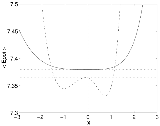
FIG. 1.: Potential energy of atoms as function of the normal coordinate, $x$, corresponding to a soft mode. Solid line: average potential energy of all atoms in the system. $\langle E_{\rm pot}(x=0)\rangle\approx 7.388\epsilon$. Dashed line: average potential energy of the 13 atoms most active in the soft mode. $\langle E_{\rm pot}(x=0)\rangle_{13}\approx 7.364\epsilon$.

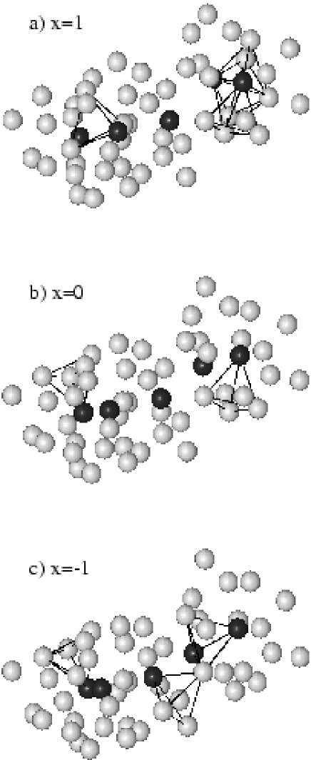
FIG. 2.: Variation of local structure in the soft mode. Black spheres: the five atoms most active in the mode. Gray spheres: geometrical neighbors of the active atoms. DS of perfect tetragonal shape ($T<0.003$) are shown. a) 7 DS, b) 2 DS, c) 4 DS.

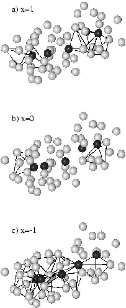
FIG. 3.: Similar to Fig. 2: DS of perfect quart-octahedral shape ($O<0.008$). a) 5 DS, b) 2 DS, c) 12 DS.

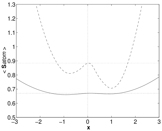
FIG. 4.: Average ideality, $S_{\rm atom}$, of the nearest neighborhood as the function of the normal coordinate, $x$, of the soft mode used in Fig. (1). Solid line: $S_{\rm atom}$ averaged over all atoms of the system. $\langle S_{\rm atom}(x=0)\rangle\approx 0.67$. Dashed line: $S_{\rm atom}$ averaged over 13 active atoms. $\langle S_{\rm atom}(x=0)\rangle_{13}\approx 0.88$.

FIG. 5.: Amplitude weighted atomic tetragonality as function of vibrational frequency, mean value (dashed line) and equidistant contour lines.

FIG. 6.: Expectation value of tetragonality with respect to vibration modes versus frequency.

FIG. 7.: Correlation of vibrational eigenvectors, ${\bf e}$, and the eigenvectors, ${\bf e_{\rm T}}$, of the tetragonality matrix as function of vibrational frequency $\nu$ and tetragonality frequency $\nu_{\rm T}$.

FIG. 8.: Correlation as in Fig. 7 for a mixed measure of tetragonality and ideality, Eq. 15.

TABLE I.: Values of ideality, tetragonality and sphericity for an atom in an ideal fcc-lattice, at the center of an icosahedron and for the glass, averaged according to Eq. 9.

	$\langle S_{\rm atom}\rangle$	$\langle T_{\rm atom}\rangle$	$\langle Sph_{\rm atom}\rangle$
fcc lattice	0.0	0.039	0.346
icosahedron	0.095	0.0015	0.325
SS-glass	0.66 $\pm$ 0.17	0.023 $\pm$ 0.005	0.358 $\pm$ 0.025

REFERENCES

- [1] W.A. Phillips (ed.), Amorphous Solids: Low Temperature Properties, Springer, Berlin 1981.
- [2] V.G. Karpov, M.I. Klinger, and F.N. Ignat’ev, Sov. Phys. JETP 57, 439, (1983).
- [3] M. A. Il’in, V. G. Karpov, and D. A. Parshin, Sov. Phys. JETP 65, 165, (1987).
- [4] U. Buchenau, Yu.M. Galperin, V.L. Gurevich, and H.R. Schober, Phys. Rev. B 43, 5039 (1991).
- [5] U. Buchenau, Yu.M. Galperin, V.L. Gurevich, D.A. Parshin, M.A. Ramos, and H.R. Schober, Phys. Rev. B 46, 2798 (1992).
- [6] V.L. Gurevich, D.A. Parshin, J. Pelous, and H.R. Schober, Phys. Rev. B 48, 16318 (1993).
- [7] S.R. Elliott, Nature 354, (1991), 445 (1991).
- [8] V.K. Malinovskii, V.N. Novikov and A.P. Sokolov, Phys. Uspekhi 163, 119 (1993).
- [9] N.N. Medvedev, Yu.I. Naberukhin, and V.A. Luchnikov, J. Struct. Chem. 35, 47 (1994).
- [10] V.A. Luchnikov, N.N. Medvedev, Yu.I. Naberukhin, and V.N. Novikov, Phys. Rev. B 51, 15569 (1995).
- [11] B¿B. Laird and H.R. Schober, Phys. Rev. Lett. 66, 636 (1991); H.R. Schober and B.B. Laird, Phys. Rev. B 44, 6746 (1991).
- [12] W. Jin, P. Vashishta, R.K. Kalia and J.P. Rino, Phys. Rev. B 48, 9359 (1993).
- [13] C. Oligschleger and H.R. Schober, Physica A 201, 391 (1993).
- [14] J. Hafner and M. Krajčí, J. Phys.: Condens. Matter 6, 4631 (1994).
- [15] P. Ballone and S. Rubini, Phys. Rev. B 51, 14962 (1995).
- [16] M. Cho, G. R. Fleming, S. Saito, I. Ohmine, and R. M. Stratt, J. Chem. Phys 100, 6672 (1994).
- [17] J. Hafner and M. Krajčí, J. Phys.: Condens. Matter 5, 2489 (1993).
- [18] H.R. Schober, C. Oligschleger, and B.B. Laird, J.Non-cryst. solids 156-158, 965 (1993).
- [19] C. Oligschleger and H.R. Schober, Phys. Rev. B 59, 811 (1999).
- [20] J.M. Ziman, Models of disorder. The theoretical physics of homogeneously disordered systems, chapter 11., Cambridge University Press, 1979.
- [21] P.H. Dederichs and R. Zeller, in Point Defects in Metals II, Springer Tracts in Modern Physics Vol. 87 (Springer Verlag, Berlin, 1980).
- [22] P. Ehrhart, K.H. Robrock, and H.R. Schober, in Physics of Radiation Effects in Crystals, R.A. Johnson and A.N. Orlov eds. (North Holland, Amsterdam, 1986).
- [23] H.R. Schober and C. Oligschleger, Phys. Rev. B 53, 11469 (1996).
- [24] W. G. Hoover, S. G. Gray, and K. W. Johnson, J. Chem. Phys. 55, 1129 (1971).
- [25] J. Fabian and P. B. Allen, Phys. Rev. Lett. 77, 3839 (1996).
- [26] D. Caprion, P. Jund, and R. Jullien, Phys. Rev. Lett. 77, 675 (1996).
- [27] P. Jund, D. Caprion, and R. Jullien, Phys. Rev. Lett. 79, 91 (1997).
- [28] P. Jund, D. Caprion, and R. Jullien, Europhys. Lett. 37, 547 (1997).
- [29] N.N. Medvedev and Yu.I. Naberukhin, J. Comput. Phys. 67, 223 (1986).
- [30] N.N. Medvedev, J. Phys.: Condens. Matter 2, 9145 (1990).
- [31] V.P. Voloshin, Yu.I. Naberukhin, and N.N. Medvedev, Mol. Simul. 4, 209 (1989).
- [32] N.N. Medvedev and Yu.I. Naberukhin, J. Non-Cryst. Solids 94, 402 (1987).
- [33] To obtain this plot, we do not make a new tesselation for each value of . The tetragonality and octahedricity are calculated for the quartets of atoms forming the DS at . This does not introduce large errors in the value of because for small displacements, the majority of atoms would be grouped in the same DS if a new tesselation is made.
- [34] H.R. Schober, to be published.