Chapter 1 Scale competition in nonlinear Schrödinger models

Yu.B. Gaididei
P.L. Christiansen
S.F. Mingaleev

Abstract

Three types of nonlinear Schrödinger models with multiple length scales are considered. It is shown that the length-scale competition universally results into arising of new localized stationary states. Multistability phenomena with a controlled switching between stable states become possible.

1 Introduction

The basic dynamics of deep water and plasma waves, light pulses in nonlinear optics and charge and energy transport in condensed matter and biophysics [1, 2, 3, 4] is described by the fundamental nonlinear Schrödinger (NLS) equation

$$i\frac{\partial}{\partial\,t}\psi+L^{2}\partial^{2}_{x}\psi+V|\psi|^{2}\psi+f(x)\psi=0\;,$$ (1.1)

where $\psi(x,t)$ is the complex amplitude of quasi-monochromatic wave trains or the wave function of the carriers. The second term represents the dispersion and $L$ is the dispersion length (e.g. in the theory of charge (energy) transfer $L^{2}=\hbar^{2}/2m$ with $m$ being an effective mass). The nonlinear term, $V|\psi|^{2}\psi$, describes a self-interaction of the quasiparticle caused either by its interaction with low-frequency excitations (phonons, plasmons, etc.) [5] or by the intensity dependent refractive index of the material (Kerr effect) [6]. The function $f(x)$ is a parametric perturbation which can be a localized impurity potential, a disorder potential, a periodic refractive index, an external electric field, etc. It is well known that as a result of competition between dispersion and nonlinearity nonlinear waves with properties of particles, solitons, arise. One can also say that this competition leads to the appearance of the new length-scale: the width of the soliton $\zeta=L/\sqrt{V}$. The presence of the parametric perturbation $f(x)$ introduces additional interplays between nonlinearity, dispersion and perturbations. In the recent paper by Bishop et al. [7] the concept of competing length-scales and time-scales was emphasized. In particular, Scharf and Bishop [8, 9] have discussed the effects of a periodic potential ($f(x)=\epsilon\cos(2\pi x/\zeta_{p})$) on the soliton of the NLS equation, and shown on the basis of an averaged NLS equation that for $\zeta_{p}/\zeta\raise 1.29167pt\hbox{$<$\kern-7.5pt\lower 4.30554pt\hbox{$\sim$}}1$ or $\raise 1.29167pt\hbox{$>$\kern-7.5pt\lower 4.30554pt\hbox{$\sim$}}1$ the periodic potential leads to a simple renormalization of the solitons and creates a ’dressing’ of the soliton. But when $\zeta_{p}\sim\zeta$ there is a crucial length-scale competition which leads to the destruction of the soliton. Another interesting example of the length-scale competition was provided by Ref. [10] where the authors showed that the propagation of intense soliton-like pulses in systems described by the one-dimensional NLS equation may be left practically unaffected by the disorder (when $f(x)$ is a Gaussian $\delta$-correlated process). This theoretical prediction has recently been confirmed experimentally using nonlinear surface waves on a superfluid helium film [11].

The goal of this paper is to extend the concept of the length-scale competition to the essentially non-integrable systems: to systems with nonlocal dispersion and to systems with unstable stationary states.

2 Excitations in nonlinear Kronig-Penney models

Wave propagation in nonlinear photonic band-gap materials and in periodic nonlinear dielectric superlattices [12, 13] consisting of alternating layers of two dielectrics: nonlinear and linear, is governed by the NLS equation

$$i\partial_{t}\psi(x,z,t) + \zeta^{2}\,(\partial^{2}_{x}+\partial^{2}_{z})\psi(x,z,t)$$ (1.2)

$$+ w\,\sum_{n}\,\delta(x-x_{n})|\psi(x,z,t)|^{2}\psi(x,z,t)=0\;,$$

where $x_{n}=n\,\ell$ is the coordinate of the n-th nonlinear layer ($\ell$ is the distance between the adjacent nonlinear layers), and it is assumed that the width $w$ of the nonlinear layer is small compared to the soliton width $\zeta$ within the layer. In this case the problem can be described by the nonlinear Kronig-Penney model given by Eq. (1.2). It was shown in Ref. [14] that the field $\psi(x,z,t)$ can be expressed in terms of the complex amplitudes $\,\psi_{n}(z,t)\equiv\psi(x_{n},z,t)$ at the nonlinear layers. The complex amplitudes $\psi_{n}(z,t)$ can be found from the set of pseudo-differential equations

$$\frac{\zeta^{2}\hat{\kappa}}{\sinh{\ell\hat{\kappa}}}(\psi_{n+1}+\psi_{n-1})-\frac{2\zeta^{2}\hat{\kappa}}{\tanh{\ell\hat{\kappa}}}\,\psi_{n}+w|\psi_{n}|^{2}\,\psi_{n}=0$$ (1.3)

with periodic boundary conditions $\psi_{n+N}=\psi_{n}$, where $N$ is the number of layers. In Eq. (1.3) the operator $\hat{\kappa}$ is defined as $\hat{\kappa}\psi=\zeta^{-1}\sqrt{-i\,\partial_{t}-\zeta^{2}\,\partial_{z}^{2}}\psi$. Equation (1.2) has an integral of motion – the norm (in nonlinear optics this quantity is often called the power) $P=\int_{-\infty}^{\infty}|\psi|^{2}dxdz$.

For the excitation pattern where the complex amplitudes are the same in all nonlinear layers, $\psi_{n}(z,t)=\Psi(z,t)$, we get

$$\sqrt{-i\partial_{t}-\zeta^{2}\,\partial^{2}_{z}}\,\tanh\left(\frac{\ell}{2\zeta}\sqrt{-i\partial_{t}-\zeta^{2}\,\partial^{2}_{z}}\right)\Psi-\frac{w}{2\zeta}|\Psi|^{2}\Psi=0\;.$$ (1.4)

Equation (1.4) clearly shows the existence and competition of two characteristic length-scales: the interlayer spacing $\ell$ and the size of the soliton in the nonlinear layer $\zeta$. When $\ell\ll\zeta$ one can expand the hyperbolic tanhence and Eq. (1.4) takes the form of usual NLS equation

$$\left(i\partial_{t}+\zeta^{2}\,\partial^{2}_{z}\right)\Psi+\frac{w}{\ell}|\Psi|^{2}\Psi=0\;.$$ (1.5)

In the opposite limit, when $\ell\gg\zeta$ and $\tanh\left(\frac{\ell}{2\zeta}\sqrt{\cdots}\right)\simeq 1$, equation (1.4) takes the form

$$\sqrt{-i\partial_{t}-\zeta^{2}\,\partial^{2}_{z}}\Psi-\frac{w}{2\zeta}|\Psi|^{2}\Psi=0\;,$$ (1.6)

which reduces, for static distribution ($\partial_{t}\Psi=0$), to the nonlinear Hilbert-NLS equation recently introduced in Ref. [15]. It is noteworthy that in contrast to usual NLS solitons, the localized solutions of the nonlinear Hilbert-NLS equation have algebraic tails [15].

It is worth to note the close relation of the problem under consideration to the theory of the long internal gravity waves in a stratified fluid with a finite depth $h$ (see e.g. [16]) which are described by the equation

$$\partial_{t}u+\frac{1}{h}\partial_{x}u+2u\partial_{x}u+T\partial^{2}_{x}u=0\;,$$ (1.7)

where $T(\cdot)$ is the singular integral operator given by

$$(Tf)(x)=\frac{1}{2h}\,p.v.\!\!\!\int\limits_{-\infty}^{\infty}\coth\left(\frac{\pi(y-x)}{2h}\right)f(y)dy$$ (1.8)

($p.v.$ means the principal value integral). In the shallow water limit ($h\rightarrow 0$) the dynamics is described by the Korteweg-de-Vries equation, $\partial_{t}u+\frac{h}{3}\partial^{3}_{x}u+2u\partial_{x}u=0$, while the Benjamin-Ono equation, $\partial_{t}u+H\partial^{2}_{x}u+2u\partial_{x}u=0$, governs the water wave motion in the deep-water limit ($h\rightarrow\infty$). Here $(Hf)(x)=\frac{1}{\pi}\,p.v.\!\!\!\int\limits_{-\infty}^{\infty}dyf(y)/(y-x)$ is the Hilbert transform.

FIGURE 1: Power $P$ of the stationary state $\psi_{n}(z,t)=e^{i\Lambda t}\phi(z)$ vs the nonlinear frequency $\Lambda$. Numerical results from Eq. (1.9) (dashed line), Padé approximation (full line) and the asymptotic relation $P\sim\Lambda^{-1/2}$ as $\Lambda\to\infty$ (dotted line).

Being interested in stationary states of the system we consider solutions of the form $\Psi(z,t)=\phi(z)\exp(i\Lambda t)$, where $\Lambda$ is the nonlinear frequency and $\phi(z)$ is the real shape function. Since Eq. (1.3) is Galilean invariant, standing excitations can always be Galileo boosted to any velocity in $z$-direction. For the shape function $\phi(z)$ we obtain a nonlinear eigenvalue problem in the form

$$\sqrt{\Lambda-\zeta^{2}\,\partial^{2}_{z}}\,\tanh\left(\frac{\ell}{2\zeta}\sqrt{\Lambda-\zeta^{2}\,\partial^{2}_{z}}\right)\phi-\frac{w}{2\zeta}\phi^{3}=0\;.$$ (1.9)

Simple scaling arguments show that in the low-frequency limit ($\Lambda\ell^{2}/\zeta^{2}\rightarrow 0$) the norm behaves in the same way as in the case of usual NLS equation (1.5): $P\sim\sqrt{\Lambda}$. When $\Lambda\ell^{2}/\zeta^{2}\rightarrow\infty$ the norm $P$ is a monotonically decreasing function: $P\sim 1/\sqrt{\Lambda}$. From the analysis of Ref. [14] follows that the norm $P(\Lambda)$ is a nonmonotonic function with a local maximum at $\Lambda_{m}\approx 1.25\zeta/\ell$ (see Fig. 1). Thus, the stationary states exist only in a finite interval, $0\leq P\leq P(\Lambda_{m})$ and for each value of norm in this interval there are two stationary states. This is an intrinsic property of the nonlinear Schrödinger superlattice system.

Discussing the stability of the stationary states satisfying Eq. (1.9), there are two sources of instability to be considered: longitudinal and transversal perturbations. The perturbations of the first type are of the same symmetry with respect to transversal degrees of freedom as the stationary states of Eq. (1.9), while the second type of perturbations breaks this symmetry. It was shown in [14] that stationary states which correspond to the branch with $dP/d\Lambda<0$ are unstable due to the longitudinal perturbations. The states with $\Lambda>(4\zeta^{2}/3\ell^{2})\sin^{2}(\pi/N)$ are, in their turn, unstable due to the transversal perturbations. Thus, one can expect stable stationary solutions for nonlinear frequencies satisfying the condition

$$\Lambda\,<\,\frac{\zeta^{2}}{\ell^{2}}\,\mbox{min}\{\frac{4}{3}\sin^{2}(\frac{\pi}{N}),\Lambda_{m}\}\;.$$ (1.10)

In particular, this means that the stationary state $\psi_{n}(z,t)=e^{i\Lambda t}\phi(z)$ can neither exist in the case of only one nonlinear layer ($\ell\rightarrow\infty$) nor in the quasi-continuum limit ($N\rightarrow\infty$). But in the latter case the system supports stationary states which are localized in both spatial directions (see Ref. [14] for details).

3 Discrete NLS models with Long-Range dispersive interactions

In the main part of the previous studies of the discrete NLS models the dispersive interaction was assumed to be short-ranged and a nearest-neighbor approximation was used. However, there exist physical situations that definitely can not be described in the framework of this approximation. The DNA molecule contains charged groups, with long-range Coulomb interaction ($1/r$) between them. The excitation transfer in molecular crystals [17] and the vibron energy transport in biopolymers [18] are due to transition dipole-dipole interaction with $1/r^{3}$ dependence on the distance, $r$. The nonlocal (long-range) dispersive interaction in these systems provides the existence of additional length-scale: the radius of the dispersive interaction. We will show that it leads to the bifurcative properties of the system due to both the competition between nonlinearity and dispersion, and the interplay of long-range interactions and lattice discreteness.

In some approximation the equation of motion is the nonlocal discrete NLS equation of the form

$$i\frac{d}{dt}\psi_{n}+\sum_{m\neq n}J_{n-m}(\psi_{m}-\psi_{n})+|\psi_{n}|^{2}\psi_{n}=0\;,$$ (1.11)

where the long-range dispersive coupling is taken to be either exponentially, $J_{n}=J\,e^{-\beta|n|}$, or algebraically, $J_{n}=J\,|n|^{-s}$, decreasing with the distance $n$ between lattice sites. In both cases the constant $J$ is normalized such that $\sum\limits_{n=1}^{\infty}J_{n}=1$ for all $\beta$ or $s$. The parameters $\beta$ and $s$ are introduced to cover different physical situations from the nearest-neighbor approximation ($\beta\rightarrow\infty,\;s\rightarrow\infty$) to the quadrupole-quadrupole ($s=5$) and dipole-dipole ($s=3$) interactions. The Hamiltonian $H=\sum\limits_{n,m}J_{n-m}|\psi_{n}-\psi_{m}|^{2}-\frac{1}{2}\sum\limits_{n}|\psi_{n}|^{4}$, which corresponds to the set of equations (1.11), and the number of excitations $N=\sum\limits_{n}|\psi_{n}|^{2}$ are conserved quantities.

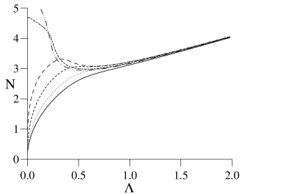
FIGURE 2: Number of excitations, $N$, versus frequency, $\Lambda$, found numerically from Eq. (1.12) for $s=\infty$ (full), 4 (dotted), 3 (short-dashed), 2.5 (long-dashed), 2 (short-long-dashed), 1.9 (dashed-dotted).

We are interested in stationary solutions of Eq. (1.11) of the form $\psi_{n}(t)=\phi_{n}\exp(i\Lambda t)$ with a real shape function $\phi_{n}$ and a frequency $\Lambda$. This gives the governing equation for $\phi_{n}$

$$\Lambda\phi_{n}=\sum_{m\neq n}J_{n-m}(\phi_{m}-\phi_{n})+\phi_{n}^{3}\;,$$ (1.12)

which is the Euler-Lagrange equation for the problem of minimizing $H$ under the constraint $N=constant$.

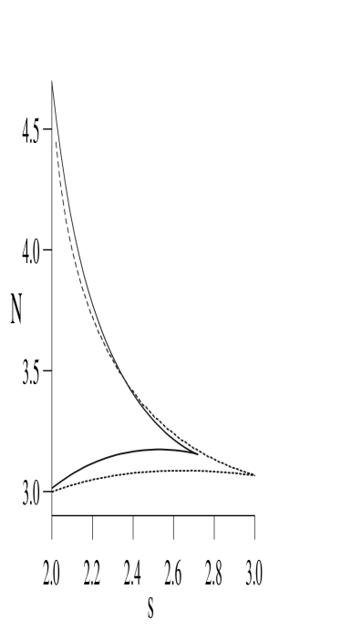
FIGURE 3: Shows endpoints of the bistability interval for $N$ versus dispersion parameter $s$. For $s=s_{cr}$ the endpoints coalesce. Analytical dependence (full) gives $s_{cr}\simeq 2.72$. Numerical dependence (dashed) gives $s_{cr}\simeq 3.03$.

Figure 2 shows the dependence $N(\Lambda)$ obtained from direct numerical solution of Eq. (1.12) for algebraically decaying $J_{n-m}$. A monotonic function is obtained only for $s>s_{cr}$. For $2<s<s_{cr}$ the dependence becomes nonmonotonic (of ${\cal N}$-type) with a local maximum and a local minimum. These extrema coalesce at $s=s_{cr}\simeq 3.03$. For $s<2$ the local maximum disappears. The dependence $N(\Lambda)$ obtained analytically using the variational approach is in a good qualitative agreement with the dependence obtained numerically (see [15]). Thus the main features of all discrete NLS models with dispersive interaction $J_{n-m}$ decreasing faster than $|n-m|^{-s_{cr}}$ coincide qualitatively with the features obtained in the nearest-neighbor approximation where only one stationary state exists for any number of excitations, $N$. However in the case of long-range nonlocal NLS equation (1.11), i.e. for $2<s<s_{cr}$, there exist for each $N$ in the interval $[N_{l}(s),N_{u}(s)]$ three stationary states with frequencies $\Lambda_{1}(N)<\Lambda_{2}(N)<\Lambda_{3}(N)$. In particular, this means that in the case of dipole-dipole interaction ($s=3$) multiple solutions exist. It is noteworthy that similar results are also obtained for the dispersive interaction of the exponentially decaying form. In this case the bistability takes place for $\beta\,\leq\,1.67$. According to the theorem which was proven in [19], the necessary and sufficient stability criterion for the stationary states is $dN/d\Lambda>0$. Therefore, we can conclude that in the interval $[N_{l}(s),N_{u}(s)]$ there are only two linearly stable stationary states: $\Lambda_{1}(N)$ and $\Lambda_{3}(N)$. The intermediate state is unstable since $dN/d\Lambda<0$ at $\Lambda=\Lambda_{2}$.

At the end points ($\Lambda(N_{l})$ and $\Lambda(N_{u})$) the stability condition is violated, since $(dN/d\Lambda)_{s}$ vanishes. Constructing the locus of the end points we obtain the curve that is presented in Fig. 3. This curve bounds the region of bistability. It is analogous to the critical curve in the van der Waals’ theory of liquid-vapor phase transition [20]. Thus in the present case we have a similar phase transition like behavior where two phases are the continuum states and the intrinsically localized states, respectively. The analog of the temperature is the dispersive parameter $s(\beta)$.

FIGURE 4: Shapes of three stationary states for $s=2.5$ and $N=3.1$. The stable: $\Lambda=0.21$ (full), $\Lambda=0.74$ (long-dashed). The unstable: $\Lambda=0.57$ (short-dashed).

The shapes of three stationary states in the interval of bistability differ significantly (see Fig. 4). The low frequency states are wide and continuum-like while the high frequency solutions represents intrinsically localized states with a width of a few lattice spacings. It can be obtained [15] that the inverse widths of these two stable states are $\alpha_{1}\,\approx\,\left(N/8J\right)^{1/(s-2)}=\left(N/8J\right)^{\ln\xi/(1-2\ln\xi)},\;\;\;\alpha_{3}\,\approx\,\ln\left(N/J\right)$ with $\xi=\exp(1/s)$ being the characteristic length scale of the dispersive interaction which is defined as a distance (expressed in lattice spacings) at which the interaction decreases in two times. It is seen from these expressions that the existence of two so different soliton states for one value of the excitation number, $N$, is due to the presence of two different length scales in the system: the usual scale of the NLS model which is related to the competition between nonlinearity and dispersion (expressed in terms of the ratio $N/J$ ) and the range of the dispersive interaction $\xi$.

FIGURE 5: Switching from continuum-like to discrete state for $\beta=1$. The initial state $\phi_{n}$ has the frequency $\Lambda\simeq 0.31$ and $N=3.6$. The time evolution of $|\psi_{n_{0}}(t)|^{2}$ when a phase torsion is applied to the center site with $\theta=0.261$ (lower curve) and $\theta=0.262$ (upper curve), respectively; inset shows time evolution of $|\psi_{n}(t)|^{2}$ for $\theta=0.262$.

FIGURE 6: Switching from discrete to continuum-like state for $\beta=1$. The initial state $\phi_{n}$ has the frequency $\Lambda\simeq 1.423$ and $N=3.6$. Same as Fig.5 with $\theta=-0.490$ (upper curve) and $\theta=-0.491$ (lower curve), respectively; inset shows time evolution of $|\psi_{n}(t)|^{2}$ for $\theta=-0.491$ (only a part of a larger system is shown).

Having established the existence of bistable stationary states in the nonlocal discrete NLS system, a natural question that arises concerns the role of these states in the full dynamics of the model. In particular, it is of interest to investigate the possibility of switching between the stable states under the influence of external perturbations, and to clear up what type of perturbations can be used to control the switching. Switching of this type is important for example in the description of nonlinear transport and storage of energy in biomolecules like the DNA, since a mobile continuum-like excitation can provide action at distance while the switching to a discrete, pinned state can facilitate the structural changes of the DNA [21]. As it was shown recently in [22], switching will occur if the system is perturbed in a way so that an internal, spatially localized and symmetrical mode (’breathing mode’) of the stationary state is excited above a threshold value.

We will in sequel mainly discuss the case when the matrix element of excitation transfer, $J_{n-m}$, decreases exponentially with the distance $|n-m|$. For $\beta=1$ the multistability occurs in the interval $3.23\,\leq\,N\,\leq\,3.78$. It is worth noticing, however, that the scenario of switching described below remains qualitatively unchanged for all values of $\beta\,\leq\,1.67$, and also for the algebraically decaying dispersive coupling with $2\,\leq\,s\,\leq\,3.03$.

An illustration of how the presence of an internal breathing mode can affect the dynamics of a slightly perturbed stable stationary state is given in Figs. 5 and 6. To excite the breathing mode, we apply a spatially symmetrical, localized perturbation, which we choose to conserve the number of excitations in order not to change the effective nonlinearity of the system. The simplest choice, which we have used in the simulations shown here, is to kick the central site $n_{0}$ of the system at $t=0$ by adding a parametric force term of the form $\theta\delta_{n,n_{0}}\delta(t)\psi_{n}(t)$ to the left-hand-side of Eq. (1.11). As can easily be shown, this perturbation affects only the site $n_{0}$ at $t=0$, and results in a ’twist’ of the stationary state at this site with an angle $\theta$, i.e. $\psi_{n_{0}}(0)=\phi_{n_{0}}\,e^{i\theta}$. The immediate consequence of this kick is, as can been deduced from the form of Eq. (1.11), that $\frac{d}{dt}\left(|\psi_{n_{0}}|^{2}\right)$ will be positive (negative) when $\theta\,>\,0$ ($\theta\,<\,0$). Thus, we choose $\theta\,>\,0$ to obtain switching from the continuum-like state to the discrete state, while we choose $\theta\,<\,0$ investigating switching in the opposite direction. We find that in a large part of the multistability regime there is a well-defined threshold value $\theta_{th}$: when the initial phase torsion is smaller than $\theta_{th}$, periodic, slowly decaying ’breather’ oscillations around the initial state will occur, while for strong enough kicks (phase torsions larger than $\theta_{th}$) the state switches into the other stable stationary state.

It is worth remarking that the particular choice of perturbation is not important for the qualitative features of the switching, as long as there is a substantial overlap between the perturbation and the internal breathing mode. We believe also that the mechanism for switching described here can be applied for any multistable system where the instability is connected with a breathing mode.

4 Stabilization of nonlinear excitations by disorder

In this section we discuss disorder effects in NLS models. Usually the investigations of disorder effects have been carried out on systems that are integrable - soliton bearing - in the absence of disorder. A common argument is that the equations, despite their exact integrability, provide a sufficient description of the physical systems to display the essential behavior. However, the more common physical situation is that integrability, and thus the exact soliton, is absent. A relevant example of such an equation is the two-dimensional (or higher-dimensional) NLS equation. The two-dimensional NLS equation is nonintegrable and possesses an unstable ground state solution which, in the presence of perturbations, either collapses or disperses (see e.g. [23, 24]).

We consider a quadratic two-dimensional lattice with the lattice spacing equal to unity. The model is given by the Lagrangian

$$L=\frac{i}{2}\sum_{n,m}\left(\psi_{n,m}^{*}\,\frac{d}{dt}\psi_{n,m}-c.c.\right)-H\;,$$ (1.13)

where

$$H = \sum_{n,m}\left(|\psi_{n+1,m}-\psi_{n,m}|^{2}+|\psi_{n,m+1}-\psi_{n,m}|^{2}\right.$$ (1.14)

$$- \left.\frac{1}{2}|\psi_{n,m}|^{4}-\epsilon_{n,m}|\psi_{n,m}|^{2}\right)$$

is the Hamiltonian of the system. In Eqs. (1.13) and (1.14) $(n,m)$ is the lattice vector ($n$ and $m$ are integer). The first two terms in Eq. (1.14) correspond to the dispersive energy of the excitation, the third term describes a self-interaction of the excitation and the fourth term represents diagonal disorder in the lattice. Here the random functions $\epsilon_{n,m}$ are assumed to have Gaussian distribution with the probability $p(\epsilon_{n,m})=\frac{1}{\eta\sqrt{\pi}}\exp[-(\epsilon_{n,m}/\eta)^{2}]$ and have the autocorrelation function $\langle\epsilon_{n,m}\epsilon_{n^{\prime},m^{\prime}}\rangle=\eta^{2}\delta_{n\,n^{\prime}}\delta_{m\,m^{\prime}}$, where the brackets $\langle....\rangle$ denote averaging over all realizations of the disorder. From the Lagrangian (1.13) we obtain the equation of motion for the excitation function in the form

$$i\frac{d}{dt}\psi_{m,n} + (\psi_{m,n-1}+\psi_{m,n+1}+\psi_{m+1,n}+\psi_{m-1,n}-4\psi_{m,n})$$ (1.15)

$$+ |\psi_{m,n}|^{2}\psi_{m,n}+\epsilon_{m,n}\psi_{m,n}=0\;.$$

Equation (1.15) conserves the norm $N=\sum\limits_{n,m}|\psi_{n,m}|^{2}$ and the Hamiltonian $H$.

We are interested in the stationary solutions of Eq. (1.15) of the form

$$\psi_{n,m}(t)=\phi_{n,m}\exp(i\Lambda t)\;,$$ (1.16)

with a real shape function $\phi_{n,m}$ and a nonlinear frequency $\Lambda$.

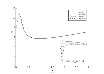
FIGURE 7: The norm $N$ versus nonlinear frequency $\Lambda$ for various disorder strengths $\eta$. Homogeneous case $\eta=0$ (solid line), $\eta=0.04$ (dotted line), $\eta=0.07$ (dashed-dotted line) and $\eta=0.1$ (dashed line).

Equation (1.15) together with Eq. (1.16) constitute a nonlinear eigenvalue problem which can be solved numerically using the techniques described in Ref. [25]. The dependences $N(\Lambda)$ in the absence and in the presence of disorder are shown in Fig. 7. It has previously been shown [26, 27, 19, 28] that the linear stability of the stationary states in the discrete case is determined by the condition $dN/d\Lambda>0$. Thus, in the case without disorder (solid curve in Fig. 7) the low-frequency ($0\leq\Lambda\leq\Lambda_{min}=1.088$) nonlinear excitations in the discrete two-dimensional NLS model are unstable. It is important that in the continuum limit ($\Lambda\rightarrow 0$) the norm $N(\Lambda)$ tends to the non-zero value $N_{c}\simeq 11.7$.

Other lines in Fig. 7 show the dependence $N$ on $\Lambda$ for the stationary solutions of Eq. (1.15) in the presence of disorder. The results have been obtained as averages of $150$ realizations of the disorder. Several new features arise as a consequence of the disorder. In the continuum limit ($\Lambda\rightarrow 0$) we no longer have $N=N_{c}$ with $dN/d\Lambda=0$. Instead we have $N\rightarrow 0$ with $dN/d\Lambda>0$ signifying that the disorder stabilizes the excitations in the low-frequency limit. The disorder creates a stability window such that a bistability phenomenon emerges. Consequently there is an interval of the excitation norm in which two stable excitations with significantly different widths have the same norm.

Furthermore, we see that the disorder creates a gap at small $\Lambda$ in which no localized excitations can exist, and that the size of this gap apparently is increased as the variance of the disorder is increased. It is also clearly seen that as $\Lambda$ increases (decreasing width) the effect of the disorder vanishes so that the very narrow excitations are in average unaffected by the disorder. It is important to stress that this is an average effect, because for each realization of the disorder the narrow excitation will be affected. The narrow excitation will experience a shift in the nonlinear frequency equal to the amplitude of the disorder at the position of the excitation.

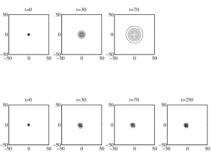
FIGURE 8: Evolution of an initial excitation of the norm $N=10.4402$ without disorder (upper part) and with disorder strength $\eta=0.1$ (lower part).

The bistability we observe in Fig. 7 occurs due to the competition between two different length scales of the system: one length scale being defined by the relation between the nonlinearity and the dispersion, while the other length scale being defined by the disorder. A similar effect was observed by Christiansen et al. [29] for the one-dimensional discrete NLS equation with a quintic nonlinearity. The latter is quite natural because as it is well known (see e.g. [30]) the properties of the two-dimensional NLS model with a cubic nonlinearity are similar to the properties the one-dimensional NLS equation with a quintic nonlinearity.

Having studied the stationary problem it is vital to compare the results to full dynamical simulations. Therefore we carry out a numerical experiment launching a pulse in a system governed by Eq. (1.15). Specifically, stationary solutions (1.16) of Eq. (1.15) with $\Lambda=0.14$ (after reducing the amplitude of these solutions by $5$%) were used as initial conditions of the dynamical simulations. Examples of the described experiment are shown in Fig. 8. As is seen the pulse behavior in the absence of disorder and in the presence of disorder (we presented here a realization corresponding to the disorder variance $\eta=0.1$) differs drastically. While the pulse rapidly disperses in the ideal system (the contour plot for $t=250$ is absent because the pulse width is of the system size), the process is arrested in the disordered system. After some transient behavior the excitation stabilizes and attains an approximately stationary width. The dynamical simulations thus support the conclusion that otherwise unstable excitations are stabilized by the presence of disorder in the low frequency limit.

Analytical theory of soliton states in disordered NLS models based on the collective coordinate approach and on the Rice’s theorem from the theory of random processes [31] is presented in Refs. [29] and [32].

5 Summary

In summary we have shown that the presence of competing length scales leads to multistability phenomena in nonlinear Schrödinger models. We have analyzed three types of the NLS models. The nonlinear Schrödinger-Kronig-Penney model presents an example where two competing length scales exist: the width $\zeta$ of the soliton in the nonlinear Schroödinger equation and the interlayer spacing $\ell$. Due to the interplay between these two length scales the localized stationary states exist only in a finite interval of the excitation power. Two branches of stationary states exist but only the low-frequency branch is stable.

In discrete nonlinear Schrödinger models with long-range dispersive interactions there exist three types of length scales: the soliton width, the lattice spacing and the radius of the dispersive interaction. Here the competition of the length scales provides the existence of three branches of stationary states. Two of them: low-frequency branch which contains continuum-like excitations and high-frequency one with intrinsically localized excitations, are stable. It is shown that a controlled switching between narrow, pinned states and broad, mobile states is possible. The particular choice of perturbation is not important for the qualitative features of the switching, as long as there is a substantial overlap between the perturbation and the internal breathing mode. The switching phenomenon could be important for controlling energy storage and transport in DNA molecules.

Considering nonlinear excitations in two-dimensional discrete nonlinear Schrödinger models with disorder it was found that otherwise unstable continuum-like excitations can be stabilized by the presence of the disorder. For the very narrow excitations the disorder has no effect on the averaged behavior. Bistability which was observed in this case is very similar to the bistability that occurs in nonlocal NLS models. Here the bistability arises on similar grounds because of competition between the solitonic length scale and the length scale defined by the disorder.

Acknowledgments:

Yu.B.G. thanks MIDIT, the Technical University of Denmark for the hospitality. Yu.B.G. and S.F.M. acknowledge support from the Ukrainian Fundamental Research Fund under grant 2.4/355.

Bibliography

- [1] Future Directions of Nonlinear Dynamics in Physical and Biological Systems, edited by P. L. Christiansen, J. C. Eilbeck, and R. D. Parmentier (Plenum Press, New York, 1993).
- [2] Nonlinear Coherent Structures in Physics and Biology, edited by K. H. Spatschek and F. G. Mertens (Plenum Press, New York, 1994).
- [3] Nonlinear Klein-Gordon and Schrödinger Systems: Theory and Applications, edited by L. Vázquez, L. Streit, and V. M. Pérez-Garcia (World Scientific, Singapore, 1996).
- [4] H. Hasegawa and Y. Kodama, Solitons in Optical Communications (Claredon Press, Oxford, 1995).
- [5] J. C. Eilbeck, P. S. Lomdahl, and A. C. Scott, Physica D 16, 318 (1985).
- [6] A. C. Newell and J. V. Moloney, Nonlinear Optics (Addison-Wiley, Amsterdam, 1992).
- [7] A. R. Bishop, D. Cai, N. Grønbech-Jensen, and M. I. Salkola, in Fluctuation phenomena: disorder and nonlinearity, edited by A. R. Bishop, S. Jiménez, and L. Vázquez (World Scientific, Singapore, 1995), p. 316.
- [8] R. Scharf and A. R. Bishop, Phys. Rev. E 47, 1375 (1993).
- [9] R. Scharf, Chaos, Solitons and Fractals 5, 2527 (1995).
- [10] Y. S. Kivshar, S. A. Gredeskul, A. Sánchez, and L. Vázquez, Phys. Rev. Lett. 64, 1693 (1990).
- [11] V. A. Hopkins et al., Phys. Rev. Lett. 76, 1102 (1996).
- [12] Photonic Band Gaps and Localization, edited by C. M. Soukoulis (Plenum Press, New York, 1993).
- [13] Photonic Band Gap Materials, edited by C. M. Soukoulis (Kluwer Academic Publishers, Dordrecht / Boston / London, 1996).
- [14] Y. B. Gaididei, P. L. Christiansen, K. Ø. Rasmussen, and M. Johansson, Phys. Rev. B 55, 13365R (1997).
- [15] Y. B. Gaididei, S. F. Mingaleev, P. L. Christiansen, and K. Ø. Rasmussen, Phys. Rev. E 55, 6141 (1997).
- [16] T. Kubota, D. R. Ko, and D. Dobbs, J. Hydronaut. 12, 157 (1978).
- [17] A. S. Davydov, Theory of Molecular Excitons (Plenum, New York, 1971).
- [18] A. C. Scott, Phys. Rep. 217, 1 (1992).
- [19] E. W. Laedke, K. H. Spatschek, and S. K. Turitsyn, Phys. Rev. Lett. 73, 1055 (1994).
- [20] L. D. Landau and E. M. Lifshitz, Statistical Physics (Pergamon Press, London, 1959).
- [21] S. Georghiou, T. D. Bradrick, A. Philippetis, and J. M. Beechem, Biophysical J. 70, 1909 (1996).
- [22] M. Johansson, Y. Gaididei, P. L. Christiansen, and K. Ø. Rasmussen, Phys. Rev. E 57, 4739 (1998).
- [23] J. J. Rasmussen and K. Rypdal, Phys. Scr. 33, 481 (1986).
- [24] K. Rypdal and J. J. Rasmussen, Phys. Scr. 33, 498 (1986).
- [25] P. L. Christiansen et al., Phys. Rev. B 54, 900 (1996).
- [26] V. K. Mezentsev, S. L. Musher, I. V. Ryzhenkova, and S. K. Turitsyn, Pis’ma Zh. Eksp. Teor. Fiz. 60, 815 (1994), [ JETP Lett. 60, 829 (1994) ].
- [27] E. W. Laedke et al., Pis’ma Zh. Eksp. Teor. Fiz. 62, 652 (1995), [ JETP Lett. 62, 677 (1995) ].
- [28] E. W. Laedke, O. Kluth, and K. H. Spatschek, Phys. Rev. E 54, 4299 (1996).
- [29] P. L. Christiansen et al., Phys. Rev. B 56, 14407 (1997).
- [30] O. Bang, J. J. Rasmussen, and P. L. Christiansen, Nonlinearity 7, 205 (1994).
- [31] O. Krée and C. Soize, Mathematics of random phenomena (Reidel, Dordrecht, 1986).
- [32] Y. B. Gaididei, D. Hendriksen, P. L. Christiansen, and K. Ø. Rasmussen, Phys. Rev. B 58, 3075 (1998).