*

Abstract

The analysis of extensive numerical data for the percolation probabilities of incipient spanning clusters in two dimensional percolation at criticality are presented. We developed an effective code for the single-scan version of the Hoshen-Kopelman algorithm. We measured the probabilities on the square lattice forming samples of rectangular strips with widths from 8 to 256 sites and lengths up to 3200 sites. At total of more than $10^{15}$ random numbers are generated for the sampling procedure. Our data confirm the proposed exact formulaes for the probability exponents conjectured recently on the base of 2D conformal field theory. Some preliminary results for 3D percolation are also discussed.

1 Introduction

Percolation is a quite common phenomena in nature. Among known examples there are epidemic diseases of garden trees, forest fires, the process of espresso preparation, Ising spins at criticality, etc. [1]. Ising spins are correlated with probability $p=1-\exp(-2J/k_{B}T)$ ($J$ is coupling constant, $k_{B}$ - Boltzmann factor and $T$ - temperature) and clusters of parallel spins percolate at the critical temperature $T_{c}$ [2].

Percolation is the simplest example of a critical phenomenon. Scaling relations for infinite lattices were developed in the same way as for the Ising model [3]. Mapping of the percolation model onto a $q=1$ state Potts model [2] gave a way to predict critical exponents for percolation in two dimensions using techniques of Conformal Field Theory (CFT) or of Coulomb gas representation.

In the last few years, new insights into the properties of percolation clusters on infinite lattices at the critical concentration have been developed. First of all, Langlands and coauthors found numerically [4] that the probability of a cluster spanning the lattice horizontally is an universal function of the aspect ratio only, and does not depend on the lattice symmetry or on the type of percolation (see also [5]).

Second, Aizenman proved that there could be more than one incipient spanning cluster in two-dimensional critical percolation [6]. His results were in contradiction with a wide-spread belief that the percolation cluster is unique (see, for example [7]). Numerical results for percolation in a strip demonstrated that there could be more than one cluster spanning the short direction in a strip [8]. Later Aizenman’s proposal was supported numerically for the case of bond percolation [9] (see also [10]).

Finally, Cardy conjectured an exact form for the probability that $k$ clusters span a large strip or open cylinder of aspect ratio $r$, in the limit when $k$ is large [11]. His result is in a complete agreement with the Aizenman theorem.

The assumptions of conformal field theory are not rigorously established, and it remains important to perform precise numerical tests of the theory. I present here an extensive numerical verification of Cardy’s proposal. The numerical data were obtained in collaboration with Sergey Kosyakov [9, 12, 31].

In Section 2 some known facts on percolation probabilities are shortly reviewed. Spanning probability are discussed in Section 3. Most recent findings on the multiplicity of incipient spanning clusters (ISC), are discussed in Section 4, where our previously published results for the ISC probabilities in bond percolation are compared with the proposed exact result. The computational method is described in the Section 5. New results for the finite size corrections of spanning probabilities in a strip geometry with up to 819200 sites are presented in Sections 6 and 7 for open boundaries and cylinder geometry. Preliminary results for the spanning probabilities in a simple cubic critical percolation with the samples with up to 1900544 sites are presented in Section 8. All averages were done using $10^{8}$ strips in all geometries investigated. Discussion and acknowledgements finish the paper.

2 Percolation

Figure 1: Example of a prime lattice and its dual. Closed bonds of the prime lattice are denoted by bold full lines, and those of the dual lattice by bold dashed lines. Open prime bonds are plotted with thin full lines. Open dual bonds are not shown.

The simplest model of percolation is bond percolation on the square lattice. Let us consider a two dimensional (2D) rectangle with an infinite number of sites $L$ in both (vertical and horizontal) directions. The probability for the bond to be occupied (or placed, or black) is equal to $p$, $0\leq p\leq 1$. Consequently, the probability for the bond to be open (or removed, or white) is equal to $q=1-p$. If all bonds are closed (that is $p=1$) the left side is connected with the right one by closed bonds. That is closed, paths from the left boundary to the right boundary exist. Clearly, if all bonds are open ones ($p=0$) there is no way to go by closed bonds through the rectangle. It appears that there is some value of the probability $p_{c}$ dividing these two possibilities. The value of critical probability $p_{c}$ is equal to $1/2$ for bond percolation in two dimensions [13, 14]. This can be seen from the self-duality of the 2D square lattice.

The dual lattice is constructed placing open bonds across the closed bonds on the prime lattice, and by drawing closed dual bonds across the open prime bonds. An example configuration is plotted in Fig. 1. It is clear from the construction that the number of closed prime bonds is equal to the number of open dual bonds. If $p$ is the probability that a bond is closed on the prime lattice, then $q=1-p$ is the probability that the chosen bond be closed on the dual lattice. For a given probability $p$ of closed bonds, let us denote by $P_{h}(p)$ the probability that there is a path of connected closed bonds connecting left and right sides of the prime lattice. That is $P_{h}(p)$ is the probability of a cluster spanning the lattice horizontally. By $P_{v}^{*}(q)$ we will denote probability that a cluster of closed bonds spans the dual lattice vertically for a given probability $q$ of closed dual bonds. Two relations follows

$$P_{h}(p)+P_{v}^{*}(q) = 1$$

$$P_{v}(p)+P_{h}^{*}(q) = 1.$$ (1)

The prime and dual lattices are identical in this construction. Therefore, the percolation threshold should be at $p_{c}=q_{c}$, i.e. $p_{c}=1/2$. A strong proof of that statement is the main subject of Kesten’s book [14].

For the finite system with square size $L\times L$ the probability $P_{h}(p;L)$ of a horizontal crossing is shown on Fig. 2 as a function of $p$ for several $L$. The slope of this curve grows with the lattice size $L$ as $L^{1/\nu}$, $\nu$ being the correlation length exponent [3]. Is is clearly visible that $P_{h}(p;L)$ approaches a step function as $L$ tends to infinity. Indeed, there are strong mathematical results [14, 15] supporting this picture.

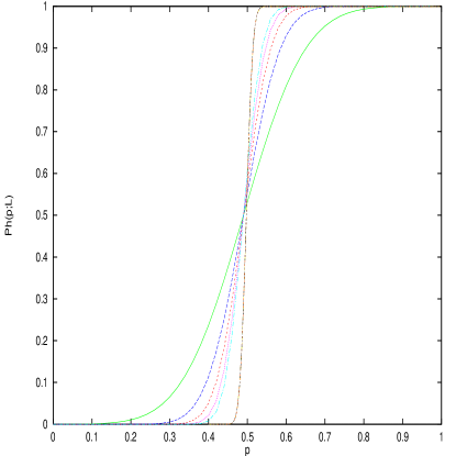
Figure 2: Spanning probability $\pi_{h}(p,L)$ as function of bond occupation probability $p$ for several values of lattice sizes $L=10,20,30,40,50$ and $200$. The larger lattice size the larger derivative of spanning probability.

What is the value of the spanning probability exactly at the percolation threshold $p_{c}$? It was believed for a long time that this value was equal to the value of the percolation threshold [3]. Indeed, this is true for the bond percolation on the square lattice. From relations (1) for the bond percolation on the infinite square lattice it is clear that

$$P_{h}(p_{c})=P_{v}^{*}(q_{c})=P_{v}(p_{c})=P_{h}^{*}(q_{c})=1/2.$$ (2)

At the same time, the real space renormalization analysis [16] are based on the relation $P_{h}(p)=p$ for the site percolation. In the last case $p_{c}\approx 0.592746$, which is fairly close to 0.5 and reasonable results for the critical exponents were computed. However it was recognized later that the value of spanning probability $P_{h}(p_{c})$ does not depend on the type of percolation as the percolation threshold does. Moreover it turns out that this value is invariant and depends only on the aspect ratio of the rectangle [4, 17, 19].

3 Incipient spanning probability

All results described in this section as well as in the following sections are obtained for critical percolation. The probability $p$ for the bond (or site) to be closed is equal to the corresponding critical value $p_{c}$ throughout the remaining text. The value of $p_{c}$ is not universal and depends on the dimensionality, lattice type (square, honeycomb, etc.) and percolation type (site, bond, etc.).

The spanning probability appears to be universal and invariant under shape transformations of the rectangle, also depends on the boundary conditions [4, 17, 19] (see also the mini review by Stauffer [20]).

Let us consider a strip with vertical size $L_{v}=L$ and horizontal size $L_{h}=rL$, where $r=L_{h}/L_{v}$ is the aspect ratio. Incipient spanning clusters connect two segments on the boundary of a macroscopically large strip. Langlands et al. [4, 19] found numerically evidence that the probability that a such cluster exists is invariant under conformal transformation. Cardy conjectured an exact formula for this probability [17] in terms of hypergeometric functions

$$P_{h}(\eta)=\frac{3\Gamma(\frac{2}{3})}{\Gamma(\frac{1}{3})^{2}}\eta^{\frac{1}{3}}\;_{2}F_{1}(\frac{1}{3},\frac{2}{3},\frac{4}{3};\eta),$$

where $\Gamma$ and ${}_{2}F_{1}$ are the gamma function and hypergeometric function respectively and $\eta=((1-k)/(1+k))^{2}$, where $k$ defines the aspect ratio $r$ of the rectangle $r=K(1-k^{2})/2K(k^{2})$ as the ratio of two complete elliptic integrals $K(u)$. The modulus $k$ is associated with the positions $(-1/k,-1,1,1/k)$ on the real axes mapped under a Schwartz-Christoffel transformation to the vertices $x_{i}$ of rectangle. Thus, the probability $P_{h}$ is just the probability that there are closed paths (Incipient Spanning Clusters) which connect the interval $(x1,x2)$ with the opposite one $(x3,x4)$. This conjecture of Cardy was confirmed numerically by Langlands, et al. [19].

A more practical form of spanning probability was developed by Ziff as series expansion in powers of $\exp(-2\pi\;r)$ [21]

$$P_{h}(r)= 2^{\frac{4}{3}}c\;(e^{-\pi r/3}-\frac{4}{7}e^{-7\pi r/3}+\frac{2}{13}e^{-13\pi r/3}...), r\geq 1$$ (3)

$$= 1-2^{\frac{4}{3}}c\;(e^{-\pi/3r}-\frac{4}{7}e^{-7\pi/3r}+\frac{2}{13}e^{-13\pi/3r}...), r\leq 1$$ (4)

where $c\equiv\Gamma(\frac{2}{3})/\Gamma(\frac{1}{3})^{2}\approx 0.566046680...$. Note, the corrections $\exp(-2\pi\;r)$ to the leading behaviour $\exp(-2\pi\;r/3)$ decay very fast with increasing $r$.

The probability that at least one cluster spans the square with open boundaries in both directions is equal to $1/2$. This value could be obtained from (3) or (4) at $r=1$.

In the case of cylinder the spanning probability along the cylinder is not known exactly. Simulations by Hovi and Aharony [22] give the value $P_{h}(1)=0.6366(8)$ for the aspect ratio $r=1$.

In a forthcoming paper [31] we compute the spanning probabilities $P_{h}(r)$ for the aspect ratio $r$ in the interval $0.25\leq r\leq 25$ for cylindrical geometry as well in the interval $0.25\leq r\leq 12.5$ in open geometry with the step $\Delta r=0.25$. The quality of these results will be discussed in the following sections.

4 Coexistence of Incipient Spanning Clusters in 2D

In the following sections we will also compute the probabilities that at least two, and even more clusters simultaneously span the lattice from left to right.

It was a common belief until recently that percolation clusters are unique on the 2D lattice. Aizenman proposed quite recently in his lecture at the Statistical Physics 19 Conference in China [23] that the number of Incipient Spanning Clusters (ISC) in 2D can be larger than one. Later he proved [6] that the probability $P(k,r;L)$ that at least $k$ ISCs span horizontally (that is along $L_{h}$) the strip $(L_{h},L_{v})=(rL,r)$ with width $L_{v}$ and horizontal length $L_{h}$ bounded

$$Ae^{-\alpha k^{2}r}\leq P(k,r;L)\leq e^{-\alpha^{\prime}k^{2}r},$$ (5)

where $\alpha$ and $\alpha^{\prime}$ are different positive constants expected to merge for an infinite lattice [6]. Indications of the existence of simultaneous clusters in two-dimensional critical percolation in the limit of infinite lattices were found in computer simulations by Sen[10] for site percolation on square lattices with helical boundary conditions and in a short strips by Hu and Lin [8] using their Monte Carlo histogram method.

We checked numerically the number of spanning clusters in the critical bond percolation model on two-dimensional square lattices [9]. We have determined the numerical values of probabilities

$$P(k,1)=\lim_{L\rightarrow\infty}P(k,1;L)$$

for $k=1,2,$ and $3$ by means of finite-size scaling. The values are given in Table 1 for the cases of free boundary conditions and periodic boundary conditions in the vertical direction (i.e. perpendicular to the spanning direction).

Table 1: Probability to have at least $k$ horizontally spanning clusters in square with free boundaries (FBC) and periodic boundaries (PBC). Bond critical percolation.

$n$	$P(k,1)$ - FBC	$P(k,1)$ - PBC
1	0.50002(2)	0.6365(1)
2	0.00658(3)	0.0020(4)
3	0.00000148(21)	0.00000014(5)

Actually, we use fully symmetric lattices, which are self dual even at finite sizes. Therefore, relations (2) holds for our finite lattices (for details, see [9]) and $P(1,1;L)\equiv 1$. In fact, the data in Table 2 support our observation. Finite size corrections for the probabilities of at least 2 incipient spanning clusters appear to be of the form $P(2,1;L)=P(2,1)+c/L^{2}$, with some constant $c$, i.e. proportional to the inverse square lattice size $L$. We found that the same finite size dependence holds also for $P(3,1;L)$ [9].

Table 2: Probabilities $P(k,1;L)$ of at least $k$ incipient spanning clusters on critical bond square lattices with size $(L,L)$ and free boundaries. Note, that the values of $P(2,1;L)$ are multiplyed by a factor $10^{3}$ and those of $P(3,1;L)$ by a factor $10^{6}$. For each lattice size $L$ the first row is the probability of horizontal spanning and the second one is the probability of vertical spanning.

$L$	$P(1,1;L)$	$P(2,1;L)\cdot 10^{3}$	$P(3,1;L)\cdot 10^{6}$
8	0.50005(5)	7.657(8)	3.40(15)
	0.50003(4)	7.660(8)	3.98(21)
12	0.50002(5)	7.084(9)	2.57(14)
	0.49995(5)	7.070(8)	2.10(13)
16	0.50003(7)	6.855(9)	1.97(17)
	0.50002(6)	6.843(8)	1.79(19)
20	0.49990(6)	6.742(8)	1.95(14)
	0.50008(5)	6.745(9)	1.72913)
30	0.49999(4)	6.650(8)	1.52(14)
	0.49996(5)	6.653(7)	1.52(12)
32	0.49999(5)	6.648(8)	1.73(12)
	0.50008(7)	6.642(8)	1.56(11)
64	0.49992(9)	6.597(9)	1.33(13)
	0.49999(6)	6.602(8)	1.51(14)

The values of probabilities in Table 1 tell us, that at criticality there is percolation in one direction with the probability equal to 1/2. Among such samples and in the case of free boundaries, in about 6 samples in 1000 there are two different clusters percolated horizontally. Finally, 1 sample in 1000000 (one million) contain at least 3 clusters spanning lattice in the given direction. The corresponding probabilities for $k>1$ are less in the case of periodic boundary conditions, that is for cylindrical geometry.

The data presented in the Table 1 appear in good agreement with the exact form of the probabilities $P(k,r)$ conjectured by Cardy using methods of conformal field theory [11]. He extend the arguments of his early paper [17] and determined the exact behaviour in the limit of infinite lattices $L\rightarrow\infty$ for the spanning probabilities $P(k,r;L)$ for large aspect ratios $r$ in the case of free boundaries

$$\lim_{L\rightarrow\infty}\ln P_{FBC}(k,r;L)\propto-\frac{2\pi}{3}k(k-\frac{1}{2})\;r,$$ (6)

as $r\rightarrow\infty$ for any $k$.

Analogously, for periodic boundaries in the vertical direction (spanning along a cylinder) he found

$$\lim_{L\rightarrow\infty}\ln P_{PBC}(k,r;L)\propto-\frac{2\pi}{3}(k^{2}-\frac{1}{4})\;r,$$ (7)

for $k\geq 2$ and $r\rightarrow\infty$, and with the different exponent for $k=1$

$$\lim_{L\rightarrow\infty}\ln P_{PBC}(1,r;L)\propto-\frac{5\pi}{24}\;r,$$ (8)

in the limit of large aspect ratio $r\rightarrow\infty$.

From the results (6-7) one could calculate ratio

$$\frac{\ln P_{FBC}(k,1)}{\ln P_{PBC}(k,1)}=\frac{k(k-\frac{1}{2})}{k^{2}-\frac{1}{4}},$$

which is $\frac{4}{5}=0.8$ for $k=2$ and $\frac{6}{7}\approx.857$ for $k=3$. Data from the Table 1 give us the values $0.808(10)$ and $0.857(20)$, respectively. This close agreement with the asymptotic form for $r\rightarrow\infty$ may be explained by the observation [11] that the corrections to the leading behaviour are of order $\exp(-2\pi r)$ (compare with expansion (4)).

The detailed numerical check of Cardy’s results (6-8) is given in the remaining sections.

5 Computational method.

Our simulations can be divided into three major parts:

Sample choosing.

There are two ways to generate a sample. The first one, is with the number of closed bonds (or sites) fixed, i.e. we choose the sample from a canonical ensemble. This method is especially convenient for the bond square percolation, when fully self-dual lattices exist even for the finite system size [9]. This eliminates not only boundary effects, but also ‘fluctuations’ of the concentration.

The second way, is with a fixed probability for a given site (bond) to be closed, i.e. sampling from a grand canonical ensemble. This method is more convenient for the Ziff hull method, for the transfer-matrix method and for the Hoshen-Kopelman algorithm we use in this work.

It is known that both methods lead to the same results in the ‘thermodynamic’ limit of infinite lattices [24]. It should be noted, that the computed averages coincide for both samples, whereas corresponding dispersions are quite different, as was found recently by Vasilyev and author [25].

To generate samples, we generate random numbers as result of XOR operations (eXclusive OR) applied to the output of two shift registers with large length. Usually, we use the pairs of legs $(p,q)$ with $(9689,471)$ and $(4423,1393)$, though some other combinations from [18] could be used as well. This give us an enormously large period of random numbers and a lack of acting correlations. Details could be found in papers [26, 27, 28, 29] and references therein.

Decomposition to clusters.

We use the Hoshen-Kopelman algorithm [30] in their original “single scan version”. That is we don’t hold the whole lattice in the memory but only the boundary column we start from, the current column and the next column. In this way, the algorithm can be named as a “dimensionality reduction” Hoshen-Kopelman algorithm. This give us the possibility to fit all data together with the instruction code within the 4 MB cache memory of Alpha workstations. So, we avoid the slowest feature of modern computers, i.e. the slowing down of data flow from CPU registers to RAM and back, typical for general simulations. The resulting speed up of simulations is a factor of about $4$.

Check of spanning.

We check spanning with the step $\Delta r$ in aspect ratio equal to $1/4$ (and even $\Delta r=1/8$ for the largest width $L=256$). Namely, the sample generation goes from right to left together with the Hoshen-Kopelman labeling. After the successful generation of $L/{\Delta r}=L/4$ sequential columns, we compare the cluster labels on the start column with the cluster labels of the current column. The resulting information is the indicator functions of the aspect ratio $I_{i}(k,r)$, where $k$ denotes the number of independent spanning clusters and $i$ is the sample number. The value of this function at a fixed value of variable $r$ is equal to 1 (there is spanning of $k$ clusters) or 0 (there is no spanning of $k$ clusters). This information is added to an output file. After $10^{6}$ scans of the strip, the file is written onto the disk and a new file is opened. The process was repeated $100$ times. So, each of $100$ files contain the probabilities $\pi_{h}(k,r;L)=10^{-6}\sum_{i=1}^{10^{6}}I_{i}(k,r)$ for the fixed value of strip width $L$. Error bars are computed over 100 such values of probabilities. It should be noted, that the probability $\pi_{h}(k,r;L)$ is the probability of exactly $k$ clusters, and we have to compute $P(k,r;L)=\sum_{j=k}^{\infty}\pi_{h}(j,r;L)$ (i.e. sum from $k$ to $\infty$) to get spanning probabilities [9] as defined in Eqs. (3,6-8).

This ends the ‘measurement’ of probabilities.

The detailed discussion of the computational methods will be published elsewhere [31].

The remaining part of the lecture is devoted to the analysis of the resulting data $P(k,r;L)$ [9, 31].

6 Finite size corrections of spanning probabilities. Free boundaries.

In this section we present an analysis of the probability $P(k,r;L)$ that at least $k$ clusters span an open strip of width $L$ at least to a distance $r$. Free boundary conditions are used throughout this section. An analysis of the probabilities with cylindrical geometry will be given in the next section.

We generate $10^{8}$ different strips of width $L_{v}=L=$8, 12, 16, 20, 24, 28, 32, 48, 64, 128, 256 sites growing up to the length of $L_{h}=rL=32000$ sites. For the site percolation at $p_{c}=0.592746$ considered here about $10^{15}$ random numbers were generated using ‘XOR’ combination of the output of two shift registers with the large lags. For some cases we repeat simulations with the linear congruential rand48 generator (compare with [4]). Comparison did not demonstrate any evidence of systematic errors.

As results of the simulations, we have data for $P(k,r;L)$. Our next task is to determine the ISC exponents. For that, we have to take $\lim_{L\rightarrow\infty}$ and determine the slope of $\ln P(k,r)$ as a function of the aspect ratio $r$. This is the first method. Another one, is to determine the slope of $\ln P(k,r;L)$ and then take the limit of large strip widths $L\rightarrow\infty$.

Theoretically, both methods should give the same result. In practice the two methods gave slightly different values which should be comparable within error bars. Coincidence of both results could be a good test on the data accuracy. Here we will demonstrate how both methods works for the spanning probability $P(1,r;L)$ for which we have exact result (3) and then we will apply both methods to the probabilities of multiple ISCs, for which only results for very large aspect ratios $r$ are known (6-8).

6.1 First method.

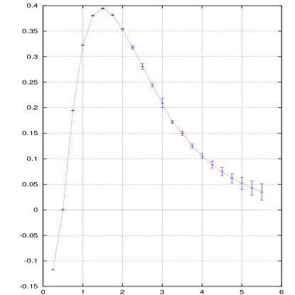
Figure 3: Coefficient $b_{0}(r)$ in the fit to the spanning probability in 2D site percolation as the function of the aspect ratio $r$. See, Eqs. 10.

First, we have to develop finite size corrections of probabilities. It is known from numerics, that the spanning probability for the site percolation on square lattices with aspect ratio $r=1$ behaves at the critical point as [5]

$$P(1,1;L)\approx P(1,1)+\frac{b_{0}}{L+L_{0}}$$ (9)

with some constants $b_{0}=0.319$ and $L_{0}=1.6$.

Our data are in agreement with this result. We found that Ziff’s proposal could be generalized [31] for any aspect ratio $r$

$$P(1,r;L)\approx P(1,r)+\frac{b_{0}(r)}{L+L_{0}(r)}$$ (10)

where $b_{0}(r)$ and $L_{0}(r)$ are now some functions of the aspect ratio $r$. $L_{0}(r)$ is a monotonic function vanishing very rapidly and can be set to zero for the aspect ratio $r\gg 2.5$. Function $b_{0}(r)$ is shown on Fig 3. It is interesting that the spanning probability for the site percolation does not depend on the lattice size for the aspect ratio close to $1/2$. We could suggest that this aspect ratio $r=1/2$ be used for the computation of percolation probability $p_{c}$ with a higher accuracy than the usual simulations at $r=1$.

Our resulting function $P(1,r)$ coincides with the exact one (3) within error bars. The linear fit to the logarithm of the resulting function $\ln P(1,r)$ in the interval $1.75\leq r\leq 5.5$ gives the slop $\epsilon_{1}=-1.0476(3)$ which is very close to Cardy’s theoretical prediction $-\pi/3=-1.047197$. To get an idea of the accuracy, the linear fit to Ziff’s approximation in the same interval was done and yielded the slope $-1.0473(1)$. So, our first method produces quite accurate data.

6.2 Second method.

Let us now compute first the slope $\epsilon_{1}(L)$ of the curves $\ln P(1,r;L)$ with respect to the aspect ratio $r$ for each strip width $L$, i.e. $\epsilon_{1}(L)$ and then take the limit

$$\lim_{L\rightarrow\infty}\epsilon_{1}(L)\rightarrow\epsilon_{1}.$$

Values of $\epsilon_{1}(L)$ are given in the Table 3. A fit to the data in the table give

$$\epsilon_{1}(L)=\epsilon_{1}+\frac{A}{L+L_{0}}=-1.04703(2)+\frac{1.3416(1)}{L+1.7558(1)},$$ (11)

with the value of $\epsilon_{1}$ equal to the exact one in 4 digits.

It is interesting that the fit of values $\epsilon_{1}(L)$ with some exponent $\theta$, i.e. with $\epsilon_{1}(L)=\epsilon_{1}+A/L^{\theta}$ yield the result $\epsilon_{1}(L)=-1.05093(1)+0.8365(2)/L^{0.8522(1)}$ with too large value of $\epsilon_{1}$ and the exponent $\theta=0.8522$ close to the irrelevant exponent, introduced by Stauffer (see, f.e. [3]) and included in the corrections to the scaling in the detailed analysis of invariance in two dimensional percolation [22]. Our data does not support this exponent but rather the expansion in powers of $1/L$ which could be effectively written as the term $A/(L+L_{0})$. Such a term was used first in a paper by Levinstein, et al. (see, f.e. [32]) in their first-time computation of the correlation length exponent and successfully used later in the context of spanning probabilities by Ziff [5] in his computation of the percolation threshold value $p_{c}=0.592746$ for the site percolation, which is the most precise value (see also [33]). We found this form to be very helpful in the data analysis.

Table 3: Slope $\epsilon_{1}(L)$ of the $\ln P(1,r;L)$ as a function of the aspect ratio $r=L_{h}/L_{v}$ for several strip widths $L_{v}=L$. Slopes are computed in the range $1.75\leq r\leq 5.5$.

$L$	$\epsilon_{1}(L)$	$\sigma$
8	-0.909926	.0001
12	-0.949355	.00003
16	-0.971482	.0001
20	-0.985734	.0001
24	-0.995344	.00005
28	-1.001989	.00008
32	-1.007151	.0001
48	-1.019926	.00004
64	-1.026430	.00007
128	-1.036904	.00007
$\infty$	-1.047032	.00002

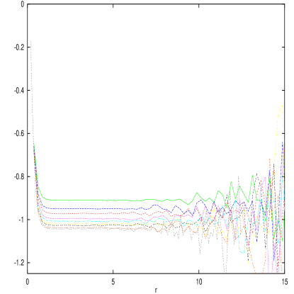
Figure 4: Derivative of the logarithm of the spanning probability $P(1,r;L)$ as a function of the aspect ratio $r$ for the strip width $L=8,12,16,24,32,48,64,128,256$ from top to bottom. Site percolation on a square open strip.

The second method could be modified in the following way. Taking the derivative of $\ln P(k,r)$ with respect to aspect ratio $r$ we get

$$\frac{d}{dr}\ln P(k,r)\propto-\frac{2\pi}{3}k(k-\frac{1}{2})=\epsilon_{k}.$$ (12)

This give us the idea the to compute $\epsilon_{k}(r,L)$ taking the numerical derivative of our data $\ln P(k,r;L)$. The result is shown on Fig. 4 for site percolation in a strip with several widths $L$. The slope of $\ln P(1,r;L)$ is constant in some region of $r$. Deviation below the left-hand value $r_{min}\approx 1.5$ is due to the corrections $\exp(-2\pi r)$ to the leading behavior as seen from Ziff’s approximation (4) and becomes negligibly small starting from $r=1.75$. Large fluctuations for aspect ratios larger than $r_{max}\approx 5.5$ is due to the small values of probabilities $P(1,r;L)$ for large $r$ and, therefore, error bars become of the size of the fluctuations (not shown on the Fig. 4 for the reason of picture clarity). The Fig. 5 shows a magnified picture with the same derivative for the values of the aspect ratio $1.75\leq r\leq 5.5$ together with the error bars.

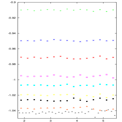
Figure 5: The same as Fig.4 for the aspect ratio in the region $1.75\leq r\leq 5.5$. Derivative of the logarithm of the spanning probability $P(1,r;L)$ for strip widths $L=8,12,16,24,32,48,64,128,256$ from top to bottom.

We now take the simple average of $\epsilon_{1}(r,L)$ over $r$ in the mentioned region and get values of $\epsilon_{1}(L)$. In the same manner as before, we could now take $\epsilon_{1}=\lim_{L\rightarrow\infty}\epsilon_{1}(L)\approx 1.0473(1)$ which is consistent with the values obtained by other methods and coincides well with the exact value.

It should be noted that the accuracy of this method is not as good as that of the previous ones because we take simple numerical derivatives, which magnify all fluctuations. Nevertheless, the method of derivatives give us clear idea on the interval $(r_{min},r_{max})$ of aspect ratio over which we can safely compute exponents. So, it is helpful as a supplement to the two methods described above.

6.3 Two and three ISC’s in an open strip.

The same analysis of the data for probability of at least two ISC leads to the exponent $\epsilon_{2}=-6.294(6)$ which is within two sigma from the exact value $-2\pi=-6.2832$. The corresponding exponent for the three ISC’s are also computed $\epsilon_{3}=-15.51(1)$. This value is well coincides with the exact value $-28/3\pi\approx-15.708$. We got relatively large deviation because the value of such probability decays very fast with the aspect ratio $r$ and practically we take averages only over the rather small interval of aspect ratio $0.5\leq r\leq 1.25$. The good agreement could be explained by the small corrections of order of $\exp(-2\pi r)$ to the leading behaviour [11].

7 Periodic boundary conditions.

Periodic boundary conditions in vertical directions lead to different values of spanning probabilities. The geometry is equivalent to an open ended cylinder with the circle length $L_{v}=L$ and “horizontal” length $L_{h}=rL$. Clusters can span from the one cylinder end to another one also rotating around the cylinder. This leads to larger values of the one cluster spanning probability than in the case of open strip described in above. Actually, we obtain a spanning probability equal to $0.6365(1)$ which is larger than $0.5$ in the case of the open strip and in a good comparison with the result of the paper [22] and more accurate. So, the spanning probability depends not only on the aspect ratio but on the boundary conditions as well [4, 19, 22]. As a consequence, the values of multiple ISC probabilities should be smaller than the corresponding ones for the open strip.

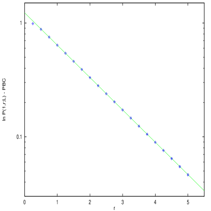
Figure 6: Spanning probability $P(1,r)$ along cylinder as function of aspect ratio $r$ denoted by open rhombs with error bars. Solid line is the best fit to probability in the interval $1.75\leq r\leq 5.5$.

We applied both methods described in the previous section to the data analysis of the spanning probability $P(1,r;L)$ along an open ended cylinder.

Using the first method we compute the slope $\epsilon_{1}$ of the logarithm of the spanning probability and get $\epsilon_{1}=-0.6547(2)$. Fig. 6 shows the probability together with the best fit.

The second method based on the slope $\epsilon_{1}(L)$ calculation for each given lattice size $L=8,12,16,20,24,28,32,36,40,48,64$ and then taking the limit of infinite lattice, finally leads to the value $\epsilon_{1}=-0.65448(5)$. Both values are very close to the exact value $-5\pi/24=-0.654498$. The second method produce much better accuracy.

Finite size corrections to the limiting values of the slope are similar to those for free boundaries. The only difference is in the finite size corrections of $\epsilon_{1}(L)$. The leading term, proportional to the inverse width vanishes, and the second power plays the main role, namely $\epsilon_{1}(L)=\epsilon_{1}-0.309(6)/L^{2}$. (We recall, that in the case of open boundaries the finite size corrections were $\epsilon_{1}(L)=\epsilon_{1}+c/(L+L_{0})$.)

The $1/L^{2}$ finite size corrections also hold for $\epsilon_{2}(L)$ and $\epsilon_{3}(L)$, whose values are $\epsilon_{2}(L)=-7.852(1)$ and $\epsilon_{3}(L)=-18.11(15)$, also quite close to the exact values $-5\pi/2=-7.8540$ and $-35\pi/6=-18.33$.

8 Incipient spanning clusters in simple cubic lattice

Aizenman, in his seminal paper [6], also proposed the ISC exponents in dimension $d$ from lower $d_{l}=2$ to upper $d_{u}=6$ critical dimensions

$$P_{h}(k,r)\propto\exp(-\alpha k^{\frac{d}{d-1}})=\exp(-\epsilon_{k}r).$$ (13)

The preliminary analysis of the data obtained for the probabilities of clusters spanning between two opposite planes of the open cube $(rL,L,L)$ at the critical site percolation threshold $p_{c}=0.3116$ [34, 35] are presented in the Table 4. We compute values of $\epsilon_{k}$ using the second method described above for system sizes $L=8,16,32,48,64$ and aspect ratio up to $r=7.25$, so some samples contain 1900544 sites. The averages were taken over $10^{7}$ such samples.

A possible fit to the data in Table 4 is $\alpha_{k}\propto-\pi(k^{1.5}-0.22k+0.11)$, which supports Aizenman proposal. We cannot exclude, nevertheless, the power in exponent being less than $d/(d-1)=1.5$.

In their preprint [36], Sen and Bhattacharjee proposed on the basis of their simulations that in the directed 3D percolation the ISC exponent depends with the same power $2$ on the number of clusters $k$. Here we compute directly exponents as the slope of the logarithm of the corresponding probabilities, whereas in the Sen and Bhattacharjee preprint only values of probabilities for one fixed aspect ratio $r=1$ were determined. We are not sure their analysis could distinguish the powers $1.5$ and $2$. We could only say that analysing our very precise data, we believe the value of power to be not larger than $1.5$.

More detailed simulations and analysis are in progress.

Table 4: Exponents $\epsilon_{k}$ depending on the number $k$ of ISC clusters in simple cubic site critical percolation.

$k$	$\epsilon_{k}$	$\sigma$
1	-2.7641	0.0004
2	-7.935	0.001
3	-14.68	0.01
4	-21.7	0.2

9 Discussion

We compute the values of the new exponents connected with the probabilities of a number of incipient spanning clusters in two dimensional percolation at criticality.

The results of comparison of the computed values with the exact ones are summarized in Table 5. Our data strongly support the exact results (6-8) for the number of incipient spanning clusters in two dimensional percolation developed by Cardy in [17, 11] and, therefore, the validity of conformal invariance for multiple spanning probabilities.

Table 5: Comparison of computed data with the exact results. Site percolation in two dimensional square lattice with free boundaries (FBC) and periodic boundaries (PBC).

	Free boundaries		Periodic boundaries
$k$	$\alpha_{k}$ Exact	$\alpha_{k}$ Comp.	$\alpha_{k}$ Exact	$\alpha_{k}$ Comp.
1	$-\frac{\pi}{3}=-1.047197$	-1.0473(2)	$-\frac{5\pi}{24}=-0.654498$	-0.65448(5)
2	$-2\pi=-6.28318$	-6.294(6)	$-\frac{5\pi}{2}=-7.8540$	-7.852(1)
3	$-5\pi=-15.70796...$	-15.51(1)	$-\frac{35\pi}{6}=-18.33$	-18.11(15)

Finite size corrections of the data computed with a high accuracy demonstrate that at criticality, corrections to all quantities analyzed depends on the inverse system size or on the inverse square size. We did not find any evidence for the irrelevant exponent $\theta_{1}=0.85$ as discussed in [22].

We stress the possibility of self duality for finite square lattices in the case of bond percolation.

We generalize finite size corrections developed by Ziff for the site percolation in a square geometry to any aspect ratio. We found that finite size scaling of the probability of cluster spanning along a strip with open boundaries is described by a nonmonotonic function $b_{0}(r)$ which vanishes at the aspect ratio $r=1/2$, or nearby.

Our preliminary data support Aizenman’s proposal for the ISC exponent in three dimensional critical percolation. More data and analysis are necessary for definite check.

10 Acknowledgments

The author would like to thank D. Stauffer, A. Aharony, R. Ziff, J. Cardy, P. Butera and J.-P. Hovi for fruitful discussions. Special thanks to S. Kosyakov together with whom most of the results were computed. The author is thankful for the invitation to D.P. Landau and for kind hospitality to the Center of Simulational Physics, University of Georgia, where this paper was finished. This work was supported in part by grants from RFBR, INTAS, Centro Volta - Landau Network and NWO.

References

- [1] A. Bunde, S. Havlin, Eds., Fractals and Disordered Systems, (Springer, Berlin, 1996)
- [2] C.M. Fortuin, P.W. Kasteleyn, Physica 57 (1972) 536
- [3] D. Stauffer, A. Aharony. Introduction to Percolation Theory, 2nd ed. (Taylor & Francis, London, 1995)
- [4] R. Langlands, C. Pichet, P. Pouliot, Y. Saint-Aubin, J. Stat. Phys. 67 (1992) 553
- [5] R.M. Ziff, Phys. Rev. Lett. 69 (1992) 2670
- [6] M. Aizenman, Nucl. Phys. B [FS] 485 (1997) 551
- [7] G. Grimmett, Percolation, (Springer, New York, 1989)
- [8] C.-K. Hu and C.-Y. Lin, Phys. Rev. Lett., 77 (1996) 8
- [9] L.N. Shchur and S.S. Kosyakov, Int. J. Mod. Phys. C 8 (1997) 473, Nucl. Phys. B (Proc. Suppl.) 63A-C (1998) 664
- [10] P. Sen, Int. J. Mod. Phys. C 7 (1996), Int. J. Mod. Phys. C 8 (1997) 229
- [11] J. Cardy, J. Phys. A 31 (1998) L105
- [12] S.S. Kosyakov, S.A. Krashakov, L.N. Shchur, Proc. Int. Conf. PDPTA’97, Las Vegas, Nevada, USA, Vol.2, 1170-1173 (Ed. H. R. Arabnia, 1997)
- [13] J. W. Essam, Rep. Prog. Phys. 43 (1980) 833
- [14] H. Kesten, Percolation theory for mathematicians, (Birkhäuser, Boston, 1982)
- [15] M. Aizenman and D.J. Barsky, Comm. Math. Phys. 108 (1987) 489
- [16] P.J. Reynolds, H.E. Stanley, and W. Klein, J.Phys. A 11 (1978) L199, Phys. Rev. B 21 (1980) 1223
- [17] J.L. Cardy, J. Phys. A 25 (1992) L201
- [18] J.R. Heringa, H.W.J. Blöte, A. Compagner, Int. J. Mod. Phys. C 3 (1992) 561
- [19] R. Langlands, P. Pouliot, Y. Saint-Aubin, Bulletin (New Series) of the American Mathematical Society, 30 (1994) 1
- [20] D. Stauffer, Physica A 242, (1997) 1
- [21] R.M. Ziff, J. Phys. A 28 (1995) 1249 , J. Phys. A 29 (1995) 6479
- [22] J.-P. Hovi, A. Aharony, Phys. Rev. E 53 (1996) 235
- [23] M. Aizenman, in proceedings of STATPHYS 19, editor Hao Bailin (World Scientific, Singapore, 1996)
- [24] R.B. Griffiths and J.L. Lebowitz, J. Math. Phys. 9 (1968) 1284
- [25] O.A. Vasilyev and L.N. Shchur, unpublished
- [26] L.N. Shchur, H.W.J. Blöte and J.R. Heringa, Physica A 241 (1997) 579
- [27] L.N. Shchur and H. Blöte, Phys. Rev. E 55 (1997) R4905
- [28] R.M. Ziff, Computers in Physics 12 (1998) 385
- [29] L.N. Shchur and P. Butera, Int. J.Mod. Phys C 9 (1998) 607
- [30] J. Hoshen, R. Kopelman, Phys. Rev. B 14 (1976) 3438
- [31] L.N. Shchur and S.S. Kosyakov, unpublished
- [32] B.I. Shklovskii, A.L. Efros, Electronic Properties of Doped Semiconductors. 5. Percolation Theory (Springer-Verlag, Berlin, 1984) pp. 95-136
- [33] R.M. Ziff, Phys. Rev. E 54 (1996) 2547
- [34] P. Grassberger, J. Phys. A 25 (1992) 5867
- [35] N. Jan and D. Stauffer, Int. J. Mod. Phys. C9 (1998) 341
- [36] P. Sen and S.M. Bhattacharjee, preprint cond-mat/9804282