Positive and negative Hanbury-Brown and Twiss correlations in normal metal–superconducting devices

Abstract

In the light of the recent analogs of the Hanbury–Brown and Twiss experiments [1] in mesoscopic beam splitters, negative current noise correlations are recalled to be the consequence of an exclusion principle. Here, positive (bosonic) correlations are shown to exist in a fermionic system, composed of a superconductor connected to two normal reservoirs. In the Andreev regime, the correlations can either be positive or negative depending on the reflection coefficient of the beam splitter. For biases beyond the gap, the transmission of quasiparticles favors fermionic correlations. The presence of disorder enhances positive noise correlations. Potential experimental applications are discussed.

In condensed matter systems, correlations effects between carriers exist either because particles interact with each other, or alternatively because the observable one considers involves a measurement on more than one particle. The characterization of current fluctuations in time constitutes a central issue in quantum transport. Noise measurements have been used to detect the fractional charge of the excitations in the quantum Hall effect [3, 4]. More recently, a fermion analog of the Hanbury–Brown and Twiss experiment [2] was achieved [1] with mesoscopic devices, obtaining a clear signature of the negative correlations expected from the Pauli principle. Here we recall rapidly the ingredients which are necessary for negative correlations and we propose a Hanbury–Brown and Twiss experiment for a fermionic system were both negative and positive (bosonic) noise correlations can be detected.

The system which is proposed (see inset of Fig. 1) consists of a junction, or beam splitter, connected by electron channels to reservoirs, which is similar to that of Ref. [6], except that the injecting reservoir is a superconductor. Because of the proximity effect at the interface between the superconductor and the normal region, electrons and holes behave like Cooper pairs provided there is enough mixing between them. While Cooper pairs are not bosons strictly speaking, an arbitrary number of theses can exist in the same momentum state, which opens the possibility for bosonic correlations. Bosonic behavior in electron systems has been previously discussed, for instance for excitons in coupled quantum wells [7], where the possibility of observing Bose condensation is in debate. On the other hand, it may be possible to detect negative correlations in adequately prepared photonic systems [8].

Negative noise correlations in branched electron circuits are the consequence of an exclusion principle, which exists for fermions (Pauli principle) or even for particles which obey Haldane’s exclusion statistics [9]. In these two situations, [10, 6, 11], ignoring thermal effects, low frequency current noise in a two–probe device is suppressed by a factor $(1-T)$, with $T$ the transmission probability. Consider first a circuit with three leads with corresponding currents and noises $I_{i}$ and $S_{i}$ labeled $i=1,2,3$, as depicted in inset of Fig. 1 (but ignoring region $4$, which we take later to be a superconductor). Assume that particles (fermions or exclusion particles) with charge $q$ are injected from $3$ with a chemical potential $\mu_{3}$ while $1$ and $2$ are kept at the same chemical potential $\mu_{1}$. Noise correlations between $1$ and $2$ can be computed by invoking that the fluctuations in $3$ [6] equal that of a composite lead $(1+2)$: at $\omega=0$, $S_{3}=S_{(1+2)}$. The definition of the noise correlations between $1$ and $2$ is:

$$S_{12}\equiv\lim_{T\rightarrow+\infty}\frac{1}{T}\int_{0}^{T}\int_{-\infty}^{+\infty}dtdt^{\prime}\langle\delta I_{1}(t)\delta I_{2}(t+t^{\prime})\rangle~{},$$ (1)

with $\delta I_{i}$ the fluctuation around the average current in $i$. The correlations $S_{12}$ are obtained by subtracting the individual noise of $2$ and $3$ from $1$: $S_{12}=[S_{3}-(S_{1}+S_{2})]/2$. For electrons and exclusion particles, a multi–terminal noise formula [6] gives:

$${S_{3}\over(\mu_{3}-\mu_{1})}={2q^{2}\over hg}\sum_{i}Tr[\tilde{s}_{(1+2),3}\tilde{s}_{(1+2),3}^{\dagger}({\bf 1}-\tilde{s}_{(1+2),3}\tilde{s}_{(1+2),3}^{\dagger})]~{},$$ (2)

were $\tilde{s}_{(1+2),3}$ is the ($2\times 1$) transmission matrix between $3$ and $(1+2)$, which is a submatrix of the scattering matrix with elements $s_{ij}$ describing the junction, ${\bf 1}$ is the two–dimensional identity matrix, and $g$ is the exclusion parameter ($g=1$ for fermions). Using current conservation, one obtains negative correlations for both fermion and exclusion particles:

$$S_{12}=-{2q^{2}\over h}{(\mu_{3}-\mu_{1})\over g}s_{13}s_{23}^{\dagger}s_{13}^{\dagger}s_{23}.$$ (3)

Minimal negative correlations $S_{12}/S_{1}=-1$ are obtained for a reflectionless, symmetric junction.

Positive correlations in systems where the injecting lead is a superconductor are now addressed. The scattering approach to quantum transport in the presence of normal–superconductor (NS) boundaries is available [12, 13, 14] so the basic steps are reviewed briefly. The fermion operators which enter the current operator are given in terms of the quasiparticle states using the Bogolubov transformation [15] $\psi_{\sigma}(x)=\sum_{n}\left(u_{n}(x)c_{n\,\sigma}-\sigma v_{n}^{*}(x)c^{\dagger}_{n\,-\sigma}\right)$, were $c^{\dagger}_{n\,\sigma}$ ($c_{n\,\sigma}$) are quasiparticle creation (annihilation) operators, $n=(i,\alpha,E)$ contains information on the reservoir ($i$) from which the particle ($\alpha=e,h$) is incident with energy $E$ and $\sigma$ labels the spin. The contraction of these two operators gives the distribution function of the particles injected from each reservoir, which for a potential bias $V$ are: $f_{ie}\equiv f(E-eV)$ for electrons incoming from $i$, similarly $f_{ih}\equiv f(E+eV)$ for holes, and $f_{i,\alpha}=f(E)$ for both types of quasiparticles injected from the superconductor ($f$ is the Fermi–Dirac distribution). Here, $eV>0$ means that electrons are injected from regions $1$ and $2$. Invoking electron–hole symmetry, the (anti)correlations of holes are effectively studied. $u_{n}(x)$ and $v_{n}(x)$ are the solutions of the Bogolubov–de Gennes equations which contain the relevant information on the reflection/transmission of electrons and holes (and their quasiparticle analogs) at the NS interface. The current operator allows to derive a general expression for the zero frequency noise correlations between normal terminals $i$ and $j$ [14, 16] which constitutes our starting point:

$$S_{ij}(0) = \frac{e^{2}\hbar^{2}}{2m^{2}}\frac{1}{2\pi\hbar}\int_{0}^{+\infty}\!\!\!dE\sum_{\alpha,\beta}f_{i\alpha}(1-f_{j\beta})\Bigl{[}A_{i\alpha j\beta}A^{*}_{i\alpha j\beta}$$ (5)

$$+B^{*}_{i\alpha j\beta}B_{i\alpha j\beta}+A_{i\alpha j\beta}B_{i\alpha j\beta}+B^{*}_{i\alpha j\beta}A^{*}_{i\alpha j\beta}\Bigr{]}~{},$$

where current matrix elements are defined by $A_{i\alpha j\beta}\equiv u_{j\beta}\partial_{x}u^{*}_{i\alpha}-u^{*}_{i\alpha}\partial_{x}u_{j\beta}$ and $B_{i\alpha j\beta}\equiv v^{*}_{j\beta}\partial_{x}v_{i\alpha}-v_{i\alpha}\partial_{x}v^{*}_{j\beta}$. The electron and hole wave functions describing scattering states $\alpha$ (particle) and $i$ (lead) are expressed in terms of the elements $s_{ij\alpha\beta}$ of the S–matrix which describes the whole NS ensemble:

$$u_{i\alpha}(x_{j}) = [\delta_{ij}\delta_{\alpha e}e^{ik_{+}x_{j}}+s_{jie\alpha}e^{-ik_{+}x_{j}}]/\sqrt{v_{+}}$$ (7)

$$v_{i\alpha}(x_{j}) = [\delta_{ij}\delta_{\alpha h}e^{-ik_{-}x_{j}}+s_{jih\alpha}e^{ik_{-}x_{j}}]/\sqrt{v_{-}}$$ (8)

where $x_{j}$ denotes the position in normal lead $j$ and $k_{\pm}$ ($v_{\pm}$) are the usual momenta (velocities) of the two branches. $S_{ij}(0)$ has been shown to have no definite sign in four–terminal noise measurements [14].

Specializing now to the NS junction connected to a beam splitter (inset of Fig. 1), $6\times 6$ matrix elements are sufficient to describe all scattering processes. At zero temperature, the noise correlations between the two normal reservoirs simplify to:

$$S_{12}(0)=\frac{2e^{2}}{h}\int_{0}^{eV}dE\sum_{i=1,2}$$ (9)

$$\times\Bigl{[}\sum_{j=1,2}\left(s^{*}_{1iee}s_{1jeh}-s^{*}_{1ihe}s_{1jhh}\right)\left(s^{*}_{2jeh}s_{2iee}-s^{*}_{2jhh}s_{2ihe}\right)$$ (10)

$$~{}~{}~{}+\sum_{\alpha=e,h}\left(s^{*}_{1iee}s_{14e\alpha}-s^{*}_{1ihe}s_{14h\alpha}\right)\left(s^{*}_{24e\alpha}s_{2iee}-s^{*}_{24h\alpha}s_{2ihe}\right)\Bigr{]}~{},$$ (11)

where the subscript $4$ denotes the superconducting lead. The first term represents normal and Andreev reflection processes [17], while the second term invokes the transmission of quasiparticles through the NS boundary. It was noted previously [16] that in the pure Andreev regime the noise correlations vanish when the junction contains no disorder: electron (holes) incoming from $1$ and $2$ are simply converted into holes (electrons) after bouncing off the NS interface. The central issue, whether disorder can induce changes in the sign of the correlations, is now addressed.

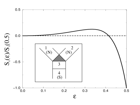
FIG. 1.: Noise correlation between the two normal reservoirs of the device (inset), as a function of the transmission probability of the beam splitter, showing both positive and negative correlations. Inset: the device consists of a superconductor ($4$)–normal ($3$) interface which is connected by a beam splitter (shaded triangle) to reservoirs ($1$) and ($2$)

Consider first the pure Andreev regime, were $eV\ll\Delta$, the superconducting gap, for which a simple model for a disordered NS junction [12] is readily available. The junction is composed of four distinct regions (see inset Fig. 1). The interface between $3$ (normal) and $4$ (superconductor) exhibits only Andreev reflection, with scattering amplitude for electrons into holes $r_{A}=\gamma\exp(-i\phi)$ (the phase of $\gamma=\exp[-i\arccos(E/\Delta)]$ is the Andreev phase and $\phi$ is the phase of the superconductor). Next, $3$ is connected to two reservoirs $1$ and $2$ by a beam splitter which is parameterized by a single parameter $0<\epsilon<1/2$ identical to that of Ref. [5]: the splitter is symmetric, its scattering matrix coefficients are real, and transmission between $3$ and the reservoirs is maximal when $\epsilon=1/2$, and vanishes at $\epsilon=0$. Electrons and holes undergo multiple reflections in central $3$ and the scattering matrix coefficient $s_{ij\alpha\beta}$ of the whole device are computed using the analogy with a Fabry–Perot interferometer.

$$s_{ii\alpha\alpha} = (x-1)(1+\gamma^{2}x^{2})/[2(1-\gamma^{2}x^{2})]$$ (12)

$$s_{ijeh} = \gamma e^{-i\phi}(1-x)(1+x)/[2(1-\gamma^{2}x^{2})]$$ (13)

$$s_{ijee} = (x+1)(1-\gamma^{2}x^{2})/[2(1-\gamma^{2}x^{2})]~{}~{}~{}~{}i\neq j~{},$$ (14)

were $x=\sqrt{1-2\epsilon}$ and the remaining coefficients of the S–matrix are found using time reversal symmetry.

Next one proceeds with the standard approximation $\gamma\simeq-i$ which applies for low biases in order to perform the energy integrals in Eq. (11):

$$S_{12}(\epsilon)=\frac{2e^{2}}{h}eV\frac{\varepsilon^{2}}{2(1-\varepsilon)^{4}}\left(-\varepsilon^{2}-2\varepsilon+1\right)~{}.$$ (15)

The noise correlations vanish at $\epsilon=0$, when conductors $1$ and $2$ constitute a two–terminal device decoupled from the superconductor, and in addition, $S_{12}$ vanishes when $\epsilon=\sqrt{2}-1$. A plot of $S_{12}$ as a function of the beam splitter transmission (Fig. 1) indicates that indeed, the correlations are positive (bosonic) for $0<\epsilon<\sqrt{2}-1$ and negative (fermionic) for $\sqrt{2}-1<\epsilon<1/2$. At maximal transmission into the normal reservoirs ($\epsilon=1/2$), the correlations normalized to the noise in $1$ (or $2$) give the negative minimal value: electrons and holes do not interfere and propagate independently into the normal reservoirs. It is then expected to obtain the signature of a purely fermionic system. When the transmission $\epsilon$ is decreased, Cooper pairs can leak in region $3$ [18] because of multiple Andreev processes. Further reducing the beam splitter transmission allows to balance the contribution of Cooper pairs with that of normal particles. Eq. (11) predicts maximal (positive) correlations at $\epsilon=1/3$: a compromise between a high density of Cooper pairs and weak transmission.

The model described above may not be convincing enough, as an ideal Andreev interface was assumed. Moreover, it does not allow to generalize the results to the case where quasiparticles in the superconductor contribute to the current. Quasiparticles have fermionic statistics, so their presence is expected to cancel the positive contribution of Cooper pairs leaking on the normal side. In particular, in the limit were $eV\gg\Delta$, one should recover fermionic correlations.

These issues bear similarities with a recent discussion of singularities in the finite frequency noise of NS junctions [19]: below the gap, a singularity exists at the Josephson frequency, while above gap there appear additional features at $eV\pm\Delta$ associated with electron and hole–like quasiparticles, which give single–particle behavior in the limit $eV\gg\Delta$. However, finite frequency noise probes the charge ($e$ or $2e$) of the carriers, while here one is probing the statistics of the effective carriers in the junction.

The energy dependence of the scattering coefficients is therefore needed to describe the correlations away from the pure Andreev regime. The numerical calculations which follow are performed using the BTK model [20], where the disordered interface between regions $3$ and $4$ (inset of Fig. 1) can be characterized by a small number of parameters: the pair amplitude is assumed to be a step function $\Delta(x)=\Delta\Theta(x)$ and a delta function potential barrier $V(x)=\hbar v_{F}Z\delta(x)$ is imposed, where $v_{F}$ the Fermi velocity and $Z\gg 1$ ($Z\ll 1$) for strong (weak) disorder. The beam splitter is taken to be similar to the previous calculation [5], assuming that the reflection/transmission of electrons does not depend significantly on the incoming energy.

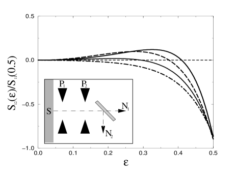
FIG. 2.: Noise correlations using an NS boundary modeled by BTK for weak disorder, $Z=0.1$: from top to bottom $eV/\Delta=0.5,0.95,1.2,1.8$. Inset: proposed device for the observation of positive/negative correlations; at the boundary of a superconductor ($S$), two point contacts ($P_{1}$) and ($P_{2}$) are connected to a semitransparent mirror ($M$)

Consider the case of weak disorder, $Z=0.1$ (Fig. 2). At weak biases, good agreement is found with the previous analytical results displayed in Fig. 1, except that for a fully transmitting splitter, the ratio of the correlations divided by the noise in region $1$ does not reach the extremal value $-1$: an early signature of disorder. When the bias is further increased but is kept below the gap, the phase accumulated in Andreev processes by electrons and holes with various energies is spread over the interval $[0,\pi/2]$: positive correlations are weaker, but they survive at low beam splitter transmission. Further increasing the voltage beyond the gap destroys completely the bosonic signature of the noise.

A strikingly different behavior is obtained for intermediate disorder at $Z=1$ (Fig. 3). First, for weak biases, the noise correlations remain positive over the whole range of $\epsilon$, with a maximum located at $\epsilon\simeq 0.43$, which is close to the case of a reflectionless splitter. This maximum becomes a local minimum for higher biases, where positive correlations remain quite robust nevertheless. Just below the gap ($eV=0.95$), correlations oscillate between the positive and the negative sign, but further increasing the bias eventually favors a fermionic behavior. Calculations for larger values of $Z$ confirm the tendency of the system towards dominant positive correlations at low biases with $S_{12}(\epsilon)/S_{1}(1/2)>1$ over a wide range of $\epsilon$ (not shown). The phenomenon of positive correlations in fermionic systems with a superconducting injector is thus enhanced by disorder at the NS boundary. Nevertheless, for strong disorder, the absolute magnitude of $S_{1}$ and $S_{12}$ becomes rather small, which limits the possibility of an experimental check in this regime.

FIG. 3.: Noise correlations using an NS boundary modeled by BTK for intermediate disorder: $Z=1$ (same biases as in Fig. 2)

An interesting feature of the present results is the fact that both positive and negative correlations are achieved in the same system. A suggestion for this device is depicted in the inset of Fig. 2. Assume that a high mobility two dimensional electron gas has a rather clean interface with a superconductor [21]. A first point contact close to the interface selects a maximally occupied electron channel, which is incident on a semi–transparent mirror similar to the one used in the Hanbury–Brown and Twiss fermion analogs [1]. A second point contact located in front of the mirror, allows to modulate the reflection of the splitter in order to monitor both bosonic and fermionic noise correlations. In addition, by choosing a superconductor with a relatively small gap, one could observe the dependence of the correlations on the voltage bias without encountering heating effects in the normal metal.

Hanbury–Brown and Twiss type experiments may become a useful tool to study statistical effects in mesoscopic devices. Here, noise correlations have been shown to have either a positive or a negative sign in the same system. Close to the boundary, a fraction of electrons and holes are correlated. This can be viewed as a finite density of Cooper pairs which behave like bosons. The presence of disorder allows in some cases to enhance the appearance of bosonic correlations. Similar studies could be envisioned in the Fractional Quantum Hall Effect (FQHE) where the collective excitations of the correlated electron fluid have unconventional statistics [9].

Discussions with the late R. Landauer, with D.C. Glattli and with M. Devoret are greatfully acknowledged.

REFERENCES

- [1] M. Henny et al., Science 284, 296 (1999); W. Oliver et al., ibid, 299 (1999).
- [2] R. Hanbury–Brown and Q. R. Twiss, Nature 177, 27 (1956).
- [3] L. Saminadayar, D. C. Glattli, Y. Jin, and B. Etienne, Phys. Rev. Lett. 79, 2526 (1997).
- [4] R. de-Picciotto, M. Reznikov, M. Heiblum, V. Umansky, G. Bunin, and D. Mahalu, Nature 389, 162 (1997).
- [5] Y. Gefen, Y. Imry and R. Landauer, Phys. Rev. Lett. 52, 139 (1984).
- [6] T. Martin and R. Landauer, Phys. Rev. B 45, 1742 (1992).
- [7] V. Negoita, D. W. Snoke and K. Eberl, Cond. Mat. 9901088 (and references therein).
- [8] R. Liu, private communication.
- [9] F.D.M. Haldane, Phys. Rev. Lett. 67, 937 (1991).
- [10] G.B. Lesovik, JETP Lett. 49, 592 (1989); M. Büttiker, Phys. Rev. Lett. 65, 2901 (1990).
- [11] S. Isakov, T. Martin and S. Ouvry, Cond. Mat. 9811391.
- [12] C.W.J. Beenakker, in Mesoscopic Quantum Physics, eds. E. Akkermans et al., p. 279 (Les Houches LXI, North Holland 1995).
- [13] B. A. Muzykantskii and D. E. Khmelnitskii, Phys. Rev. B 50, 3982 (1994).
- [14] M. P. Anantram and S. Datta, Phys. Rev. B 53, 16 390 (1996).
- [15] P.G. de Gennes, Superconductivity of Metals and Alloys, (Addison Wesley, 1966, 1989).
- [16] T. Martin, Phys. Lett. A 220, 137 (1996).
- [17] A.F. Andreev, J. Exp. Theor. Phys. 46, 1823 (1964) [Sov. Phys. JETP 19, 1228 (1964)].
- [18] See for example, A.A. Abrikosov, Fundamentals of the Theory of Metals, (North-Holland, 1988)
- [19] G. Lesovik, T. Martin and J. Torrès, Cond. Mat. 9902278; J. Torrès, G. Lesovik and T. Martin, (in preparation, 1999).
- [20] G.E. Blonder, M. Tinkham and T.M. Klapwijk, Phys. Rev. B 25, 4515 (1982).
- [21] A. Dimoulas et al., Phys. Rev. Lett. 74, 602 (1995).