Statistical-thermodynamical foundations of anomalous diffusion

Abstract

It is shown that Tsallis’ generalized statistics provides a natural frame for the statistical-thermodynamical description of anomalous diffusion. Within this generalized theory, a maximum-entropy formalism makes it possible to derive a mathematical formulation for the mechanisms that underly Lévy-like superdiffusion, and for solving the nonlinear Fokker-Planck equation.

]

I Introduction: Diffusion processes

Among the elementary processes that underly natural phenomena, diffusion is certainly one of the most ubiquitous. In an ensemble of moving elements –atoms, molecules, chemicals, cells, or animals– each element usually performs, at a mesoscopic description level, a random path with sudden changes of direction and velocity. As a result of this highly irregular individual motion, which is microscopically driven by the interaction of the elements with the medium, and of the elements with each other, the ensemble spreads out. At a macroscopic level, this collective behavior is –in contrast with the individual microscopic motion– extremely regular, and follows very well defined, deterministic dynamical laws. It is precisely this smooth macroscopic spreading of an ensemble of randomly moving elements that we associate with diffusion.

One of the first systematic observations of diffusion was made by the botanist Robert Brown in 1828. He noticed that pollen particles dispersed in water exhibit a very irregular, swarming motion. In 1905, Einstein conjectured that this “Brownian motion” is due to the interaction of pollen with the water molecules and, in fact, proved that microscopic particles suspended in a liquid “perform movements of such magnitude that they can be easily observed in a microscope, on account of the molecular motions of heat” [1]. Since then, Brownian motion is used as a synonym of diffusion.

A very suitable and very useful mathematical model for Brownian motion is provided by random walks [2]. In its simplest version, a random walker is a point particle that moves on a line at discrete time steps $\Delta t$. At each step, the walker chooses to jump to the left or to the right with equal probability, and then moves a fixed distance $x$. This stochastic process can be readily generalized, firstly, by allowing the walker to move in a many-dimensional space. In addition, time can be made continuous by associating a random duration with each jump or by introducing random waiting times between jumps. Finally, the length of each jump can be also chosen at random from a continuous set with a prescribed probability distribution.

Being a stochastic process, a random walk admits a probabilistic description in terms of probability distributions for the relevant quantities [3]. In particular, one is interested at studying the probability of finding the walker in a certain neighborhood $d{\bf r}$ of point ${\bf r}$ –in general, in a $d$-dimensional space– at time $t$, $P({\bf r},t)\ d{\bf r}$. Note that, besides its interpretation as a probability distribution, $P({\bf r},t)$ can be related to the density in an ensemble of noninteracting identical random walkers. In fact, if the ensemble contains $N$ walkers, $n({\bf r},t)=NP({\bf r},t)$ stands for the space density of walkers.

Suppose that the random walk is defined in continuous time and space, with a waiting time probability distribution $\psi(\tau)$ and such that the probability that the walker jumps from any point ${\bf r}$ to ${\bf r}+{\bf x}$ is $p({\bf x})\ d{\bf x}$. The normalization of probabilities imposes

$$\int_{0}^{\infty}\psi(\tau)\ d\tau=1,\ \ \ \ \ \ \int p({\bf x})\ d{\bf x}=1.$$ (1)

If, moreover, $\psi(\tau)$ and $p({\bf x})$ satisfy

$$\langle\tau\rangle=\int_{0}^{\infty}\tau\ \psi(\tau)\ d\tau<\infty,\ \ \ \ \langle x^{2}\rangle=\int x^{2}p({\bf x})\ d{\bf x}<\infty,$$ (2)

($x\equiv|{\bf x}|$) it can be proven that $P({\bf r},t)$ obeys the diffusion equation [2]

$$\frac{\partial P}{\partial t}=D\nabla^{2}_{\bf r}P,$$ (3)

where $D\propto\langle x^{2}\rangle/\langle\tau\rangle$ is the diffusion constant, or diffusivity. This equation has to be solved for a given initial condition $P({\bf r},0)$ with suitable boundary constraints. The density $n({\bf r},t)$ of an ensemble of noninteracting diffusing particles obeys the same equation.

A typical solution to the diffusion equation describes a density profile that, as time elapses, is smoothed out and broadens. In fact, it can be straightforwardly shown from the general solution that the width of the spatial distribution grows with time as

$$\langle r^{2}\rangle=\int r^{2}P({\bf r},t)\ d{\bf r}=2dDt,$$ (4)

where $d$ is the space dimension. Correspondingly, it can be shown that the mean square distance between the present position and the initial position of a random walk that satisfies Eq. (2) is proportional to time. This proportionality between mean square displacement and time is the fingerprint of diffusion, as it can be used experimentally, numerically, and theoretically to detect this kind of transport mechanism in a given natural process.

Though, being a form of transport, diffusion is inherently a nonequilibrium process, the large-time asymptotic dynamics of an ensemble of diffusing particles can be described in the frame of equilibrium statistical mechanics. In fact, it is expected that, for very large times, the system reaches a state of thermodynamical equilibrium with the medium –and between the particles, if they interact. In such state, the diffusing particles and the medium participate of a balanced interchange of momentum and energy, which mantains the particles in their characteristic irregular motion. Once this situation is reached, a connection between the parameters that characterize thermodynamical equilibrium and particle dynamics should exist. Einstein investigated this problem in 1905 [1], and concluded that diffusivity and temperature are proportional:

$$D=\mu k_{B}T.$$ (5)

Here $k_{B}$ is Boltzmann constant, and $\mu$ is the mobility. The mobility is defined as the inverse of the friction coefficent, in the present case, of the diffusing particles in the medium [4]. The Einstein relation, Eq. (5), provides thus the expected connection between diffusion and thermodynamical equilibrium.

Despite the omnipresence of diffusion as a transport mechanism in natural processes, a different kind of transport underlies a selected –but ever growing– class of systems. Due to various motivations most of these systems have recently attracted very much attention. They range from turbulent fluids, to chaotic dynamical systems, to genetic codes (see next section). In these systems, anomalous diffusion –a mechanism closely related to normal diffusion, but with some qualitatively different properties– drives transport processes [5]. Over the last few years, it became more and more clear that anomalous diffusion can be made naturally compatible with equilibrium thermodynamics if the Boltzmann-Gibbs formulation of thermodynamics is replaced by Tsallis’. This compatibility generalizes then the connection between normal diffusion and the usual formulation of thermodynamics. The main aim of this paper is to review this generalization, commenting on some additional related topics brought to light in recent work.

II Anomalous diffusion and Lévy flights

Any transport mechanism which, like diffusion, behaves at mesoscopic level as an isotropic random process, but which violates Eq. (4), is generally refered to as anomalous diffusion. More specifically, most of the literature on anomalous diffusion has been devoted to processes where the mean square displacement $\langle r^{2}\rangle$ varies with time as

$$\langle r^{2}\rangle\propto t^{2/z},$$ (6)

where $z$ ($\neq 2$) is the dynamic exponent, or random walk fractal dimension, of the transport process. Normal diffusion corresponds to $z=2$. For $z>2$, the growth rate of the mean square displacement is smaller than in normal diffusion, and transport is consequently said to be subdiffusive. On the other hand, for $z<2$ the mean square displacement grows relatively faster and transport is thus superdiffusive. In the following, the attention will be mainly focused on this latter case.

A Anomalous diffusion in Nature

As advanced above, anomalous diffusion occurs in a wide class of natural systems and processes. In the realm of physics, a paradigmatic example is given by particle transport in disordered media. Consider the motion of particles in a medium containing impurities, defects, or some kind of intrinsic disorder, such as in amorphous materials. Examples are disordered lattices, porous media, and dopped conductors and semiconductors. In these heterogeneous substrates, particles are driven by highly irregular forces, which determine a complex variation of the local transport coefficients. This heterogeneity can in fact induce anomalous diffusion. For instance, it has been experimentally shown that in quasi-one-dimensional ionic conductors such as hollandite (K_1.54Mg_0.77Ti_7.23O₁₆), where transport is very sensitive to the presence of impurities, the dynamic exponent is given by

$$z\approx 1+\frac{1}{\theta},$$ (7)

with $\theta$ proportional to the temperature [6].

A reasonable model for transport in heterogeneous media is provided by a random walk in a lattice with quenched disorder [5]. This disorder applies to the depth of the potential wells at each lattice site, and to the potential barriers between sites. Randomness in these parameters induces a distribution for the time that the walker spends at each site before hoping to a neighbor. Generally, this waiting time distribution, $\psi(\tau)$, behaves as $\psi(\tau)\sim\tau^{-1-\mu}$ for $\tau\to\infty$. For $\mu>1$, the first relation in Eq. (2) holds, and normal diffusion is observed. On the other hand, for $\mu<1$ the mean waiting time diverges and diffusion is anomalous. The corresponding dynamic exponent for $0<\mu<1$ is [7]

$$z=2/\mu\ \ \ (d>2),\ \ \ \ \ z=2-d+d/\mu\ \ \ (d<2).$$ (8)

A most important instance of anomalous diffusion in physics occurs in turbulent flows. In fully developed turbulence, fluid particles exhibit very irregular motion over a wide range of space and time scales. Based on empirical motivations, L. Richardson proposed in 1926 that the probability $P(R,t)$ that two fluid particles initially close to one another have a separation $R$ at time $t$ obeys the equation [8]

$$\frac{\partial P}{\partial t}=\frac{\partial}{\partial R}\left[D(R)\frac{\partial P}{\partial R}\right].$$ (9)

Comparing with (3), it is clear that the Richardson equation is a diffusion equation with space-dependent diffusivity. Its solution immediately implies $\langle R^{2}\rangle\propto t^{3}$, indicating that the relative motion of particles in fully developed turbulence corresponds to anomalous diffusion with a dynamic exponent $z=2/3$, which is well into the superdiffusive regime.

Richardson’s law has to be modified to take into account the fact that the vorticity field in a turbulent flow is intermittent [9]. This means that vorticity –and, in particular, turbulent activity and dissipation– is concentrated on a relatively small volume in the whole system, which happens to be a fractal set. Experiments [10] suggest that the fractal dimension of this set is $d_{f}=2.8\pm 0.05$. Incorporating this correction, it can be shown [11] that $\langle R^{2}\rangle\propto t^{12/(1+d_{f})}$, or

$$z=\frac{1+d_{f}}{6}\approx 0.63.$$ (10)

A somewhat more abstract form of anomalous diffusion is present in the evolution of chaotic Hamiltonian dynamical systems in phase space. Hamiltonian systems are characterized by volume conservation in phase space, as stated by the Liouville theorem. The domain occupied by a given set of initial conditions in phase space can be strongly distorted under the effect of evolution, but its volume remains constant. Mechanical processes that preserve energy are instances of Hamiltonian systems, but a huge host of systems –both continuous and discrete in time– is known to belong to the same class. Since a single Hamiltonian system can exhibit both regular and chaotic evolution by simply changing the initial condition, the dynamical geometry of its phase space is usually extremely intrincate. Zones of nested regular trajectories which alternate with chaotic regions are typically found at many scales, displaying selfsimilar structures. In the bulk of chaotic regions trajectories are extremely irregular and resemble random paths. On the other hand, when approaching the boundary with a regular region, the same trajectory can temporarily become much simpler and smoother. Consequently, as it evolves in phase space along a chaotic orbit, a Hamiltonian system alternates intermittently between zones of highly complex behavior and a regime of almost regular dynamics. Globally, this motion can be thought of as a stochastic process, and turns out to have the same statistical properties as anomalous diffusion.

A case studied in detail in the literature is the so-called Q-flow [12]. It is defined as a three dimensional velocity field

$$\begin{array}[]{ll}\dot{x}=&\partial\Psi/\partial y+\epsilon\sin z\\ \dot{y}=&\partial\Psi/\partial x+\epsilon\cos z\\ \dot{z}=&\Psi\end{array}$$ (11)

with

$$\Psi(x,y)=\sum_{j=1}^{k}\cos\left[x\cos(2\pi j/k)+y\sin(2\pi j/k)\right].$$ (12)

Here $\epsilon$ is a parameter and $k$ is an integer that determines the symmetry of the flow. The solution to Eqs. (11) is a complex trajectory that wanders in an infinite connected net of channels of width of order $\epsilon$, inside which the trajectory looks like a random contour [13]. Numerical measurements of the statistical properties of these diffusion-like trajectories show that the dynamic exponent $z$ to be associated with them fluctuates strongly as a function of $\epsilon$ [12]. For $k=6$ and $0.8<\epsilon<1.8$, $z$ varies in the interval

$$1<z<2,$$ (13)

making apparent that the motion is supperdiffusive, as in turbulence. Anomalous diffusion has also been observed in dissipative (non-Hamiltonian) dynamical systems, both in simulations and in experiments. For example, a dynamic exponent $z\approx 1.2$ has been measured in the Taylor-Couette flow[14].

As stated in the Introduction, anomalous diffusion is not restricted to physical systems. This kind of transport has in fact been detected to underly several biological processes. Some sectors of genomic DNA sequences, for instance, are known to exhibit statistical properties analogous to anomalous diffusion. To stress this correspondence, “DNA walks” have been defined [15]. DNA, which codes genetic information, is a large molecule in the form of a chain of nucleotides. Each nucleotide contains either a purine or a pyramidine base. Two purines –the adenine (A) and the guanine (G)– and two pyramidines –the cytosine (C) and the thymine (T)– are in turn present in the DNA chain. Therefore, the information code in DNA is a symbolic chain of four letters: A, C, G and T. Amazingly, within DNA only a small portion does code information for protein building (3% in the human genome) whereas other zones are noncoding, their specific role being unknown. A one-dimensional DNA walk is constructed by sequentially running over the chain of nucleotids. Each time a purine is found the walker jumps rightwards, whereas when a pyramidine is found the jump occurs leftwards. For instance,

$$\cdots\mbox{ACGCTGAGTG}\cdots\ \to\ \cdots+-+--+++-+\cdots$$

where $+$ stands for jumps to the right and $-$ stands for jumps to the left. In this DNA walk, systematic deviations from normal diffusive behavior derive from long-range correlations in the nucleotide sequence. It has been found that the DNA walk is in fact statistically identical to normal diffusion in the zones of the genomic chain that code information. On the other hand, in noncoding sequences the DNA walk is analogous to superdiffusion. In the human beta-globin chromosomal region the dynamic exponent is $z\approx 1.4$ [16].

A less involved instance of anomalous diffusion in biology appears in the flight patterns of certain birds. In particular, it has been found [17] that in the foraging behavior of the wandering albatross (Diomedea exulans) the flight-time intervals exhibit a power-law distribution. This results in a anomalous diffusive-like motion which, according to field measurements on the Bird Island, South Georgia, has a dynamic exponent $z\approx 1.2$. The kind of flight patterns observed in these seabirds is supposed to reflect a complex structure in the underlying ecosystem, especially, in the spatial distribution of the exploited environment. It has been suggested that albatrosses specialize in long journeys of random foraging, searching for patchily and unpredictably dispersed prey over several million square kilometers. As discussed in the next section, anomalous diffusion is inherently related with fractal geometry, scale-invariance, and self-similarity, which in the present example seem to drive the predator-prey dynamics.

Of course, the previous collection of examples of anomalous diffusion in Nature is not at all exhaustive, but only pretends to give a hint on the variety of systems driven by this kind of transport. For a more detailed account, the reader is refered to the review by Bouchaud and Georges [5]. This review is also an excellent reference to the mathematical treatment of anomalous diffusion, which is briefly introduced in the following.

B Random-walk models of anomalous diffusion

In view of the efficacy of random walks in modeling normal diffusion at a mesoscopic level, it is desirable to find a similar stochastic model describing anomalous diffusion. It has already been mentioned in Section II A that introducing a waiting time distribution which, for large waiting times, behaves as $\psi(\tau)\sim\tau^{-1-\mu}$ with $\mu<1$, produces the anomalous dynamic exponent given in Eq. (8). In this case $z>2$ and, therefore, transport is subdiffusive. Note that the source of anomaly in these random walks is the divergency of the average waiting time $\langle\tau\rangle$. For $\mu<1$, the long-tailed distribution $\psi(\tau)$ allows for very long waiting times with relatively high probability, violating thus the first relation in Eq. (2). These long waiting times produce an overall reduction of efficiency in the transport mechanism with respect to normal diffusion, and leads to subdiffusive behavior.

Taking into account the previous argument, in can be expected that the violation of the second of relations (2) will lead, on the other hand, to superdiffusion. In fact, having a divergent mean square displacement $\langle x^{2}\rangle$ requires the jump probability distribution $p({\bf x})$ to have a long tail for large $x$, in a sense to be made precise immediately. This long-tailed distribution would produce, with relatively high probability, very long jumps. Globally, this transport mechanism should result more efficient than normal diffusion, and superdiffusive behavior is expected.

It can be easily shown that, in $d$-dimensional space, the mean square displacement diverges if

$$p({\bf x})\sim\frac{1}{x^{d+\gamma}}$$ (14)

for large $x$, with $\gamma<2$. Note that, for such distribution, normalization requires $\gamma>0$. It is therefore to be expected that a random walk with a jump distribution $p({\bf x})\sim x^{-d-\gamma}$ with $0<\gamma<2$ does not model normal diffusion, but some kind of superdiffusive motion. Of course, a large score of functions satisfy Eq. (14), and are thus candidates to play the role of a jump distribution for a superdiffusive random walk. Among them, Lévy distributions have been studied in detail.

Lévy distributions [18] are defined through their Fourier transform, which reads

$$p({\bf k})=\int\exp(i{\bf k}\cdot{\bf x})\ p({\bf x})\ d{\bf x}=\exp(-bk^{\gamma}),$$ (15)

where $b$ is a positive constant, and $k\equiv|{\bf k}|$. Although the antitransform $p({\bf x})$ has no analytical expression, it can be shown that it satisfies Eq. (14). Moreover, if $\gamma<2$ the positivity of $p({\bf x})$ is insured. The relatively simple form of this jump distribution in the Fourier representation makes it an ideal tool for analytical manipulation. However, the main interest of Lévy functions in the mathematical theory of distributions comes from the fact that they are stable. Essentially, this means that two Lévy functions with the same Lévy exponent $\gamma$ produce, upon convolution, a third Lévy function with the same exponent. This can be readily proven in the Fourier representation, where the convolution transforms into ordinary product:

$$p_{1}({\bf k})p_{2}({\bf k}) = \exp(-b_{1}k^{\gamma})\exp(-b_{2}k^{\gamma})$$ (16)

$$= \exp[-(b_{1}+b_{2})k^{\gamma}]=p_{3}({\bf k}).$$ (17)

Lévy functions are not the only stable distributions, the Gaussian $p({\bf x})\propto\exp(-x^{2})$ being probably the best-known example. The (one-dimensional) Cauchy distribution, $p(x)\propto(1+x^{2})^{-1}$, is another instance. Stable distributions play a fundamental role in probability theory since according to the central limit theorem –which is usually stated for the Gaussian function– the addition of random variables tends to one such distribution. In particular, as P. Lévy demonstrated through his generalization of the Gaussian central limit theorem [18, 19], adding random variables with a power-law distribution as in (14) –whose second moment $\langle x^{2}\rangle$ diverges for $\gamma<2$– leads asymptotically to a Lévy distribution.

Another important property of Lévy distributions, which is reflected in its power-law large-$x$ asymptotic behavior, Eq. (14), is the absence of characteristic length scales. This implies that random walks with Lévy jump distributions have self-similar properties. In particular, it can be shown that the set of points visited by this kind of random walk is a fractal of dimension $\gamma$ [20]. As a consequence, these distributions ubiquitous in the realm of self-similarity geometry –the geometry of fractals.

A discrete-time random walk whose jump distribution is given by a Lévy function as in Eq. (15) is called a Lévy flight. It has been suggested [21] that the Fourier transform $P({\bf k},t)$ of the probability distribution of finding the walker at a given point at time $t$ satisfies the evolution equation

$$\frac{\partial P}{\partial t}({\bf k},t)=-D_{\gamma}k^{\gamma}P({\bf k},t).$$ (18)

This equation generalizes, in the Fourier representation, the diffusion equation (3). A straightforward dimensionality analysis shows that the anomalous diffusivity is $D_{\gamma}\propto b/\Delta t$, where $\Delta t$ is the time step of the random walk. In free space, equation (18) can be readily solved:

$$P({\bf k},t)=P({\bf k},0)\exp(-D_{\gamma}k^{\gamma}t).$$ (19)

For a delta-like initial condition, $P({\bf r},0)=\delta({\bf r})$, one has $P({\bf k},0)=1$ and, thus,

$$P({\bf r},t)=(2\pi)^{-d}\int\exp(-i{\bf k}\cdot{\bf r}-D_{\gamma}k^{\gamma}t)\ d{\bf k}.$$ (20)

This function remains unchanged, except for a constant factor, if both space and time are conveniently rescaled, $P(\alpha^{1/\gamma}{\bf r},\alpha t)=\alpha^{-d/\gamma}P({\bf r},t)$. Using this scale invariance, one can write

$$P({\bf r},t)=t^{-d/\gamma}\Pi(r/t^{1/\gamma}),$$ (21)

where $\Pi$ is a function of a single variable [22]. In turn, this implies

$$\langle r^{2}\rangle\propto t^{2/\gamma},$$ (22)

for $0<\gamma<2$. This result, which has been here derived for a delta-like initial distribution, can be generalized by simple superposition to more general initial conditions. It shows that a Lévy flight with $0<\gamma<2$ represents superdiffusion with a dynamic exponent $z=\gamma$. On the other hand, for power-law jump distributions with $\gamma>2$ the dynamic exponent corresponds to normal diffusion, $z=2$ (Figure 1).

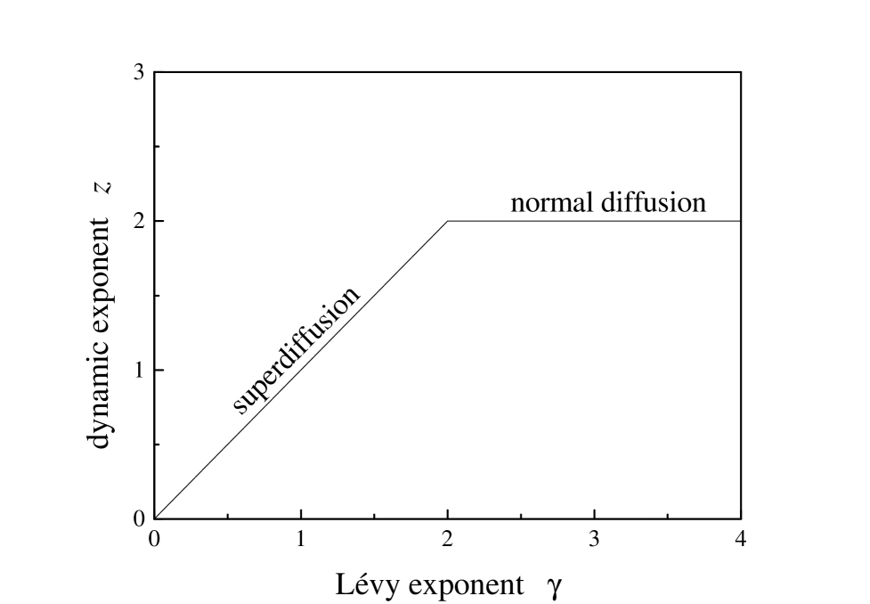
FIG. 1.: The diffusion dynamic exponent $z$ as a function of the Lévy exponent $\gamma$.

The fact that in Lévy flights the mean square displacement $\langle x^{2}\rangle$ of a single step diverges, implies –in contrast with Eq. (22)– that the mean square displacement of the walker after a certain time is, on the average over infinitely many realizations, also infinite. The arguments used to derive Eq. (22) are therefore of limited validity [21, 22], and have to be taken cum grano salis. The result (22) is expected to be valid for finite times, i.e. in a certain portion of the whole random walk, and on averages over a finite number of trajectories. The same result would be valid during a certain time if the jump distribution $p({\bf x})$ is a Lévy function in some (large) range of values of $x$, but has a cutoff for sufficently large $x$ [23]. In spite of this drawback, Lévy flights provide a very powerful tool for modeling superdiffusion because of the mathematical properties of the Lévy distributions, summarized above. They are thus a very satisfactory starting point as a model for studying the statistical mechanics of superdiffusive transport, generalizing the results outlined in the Introduction for normal diffusion.

Before passing to the discussion of superdiffusion in a statistical-mechanical frame, a comment is in order on the numerical simulation of superdiffusive random walks. Due to the cumbersome properties of Lévy distributions in real space [20], it is not convenient –in numerical calculations– to work directly with these functions. Rather, power-law distributions with the same asymptotic properties as Lévy’s, Eq. (14), are used. For instance, one can take

$$p({\bf x})=\frac{{\cal N}}{(1+x)^{d+\gamma}},$$ (23)

with ${\cal N}$ a normalization constant. The Fourier transform of these distributions behaves precisely like a Lévy distribution for small $k$, $p({\bf k})\approx 1-bk^{\gamma}$. Also, they show the same scale invariance for large $x$, wich leads to self-similar properties in the associated random walks. In Figure 2 the first $10^{4}$ points visited by a random walk in two dimensions, with the jump distribution given in (23) and $\gamma=1.5$, are shown. Note the clustered, fractal-like structure of this set of points.

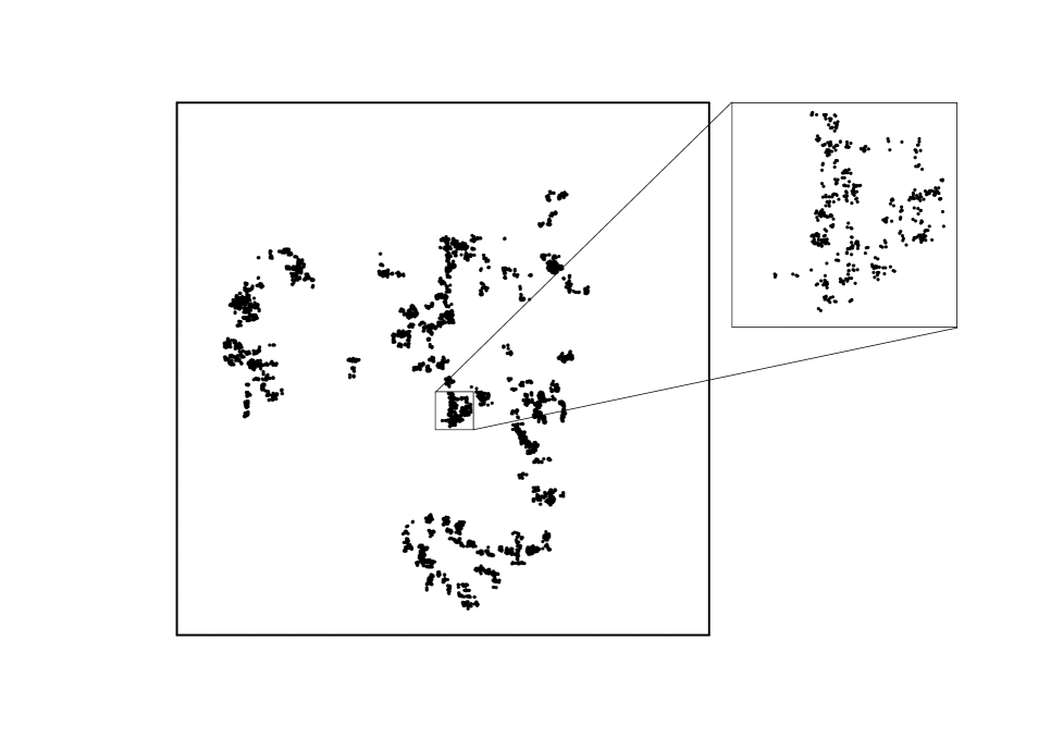
FIG. 2.: The first $10^{4}$ points visited by a two-dimensional random walk generated by a power-law jump distribution with exponent $\gamma=1.5$, starting at the center of the main frame. The amplification illustrates the self-similar properties of this process.

III Maximum-entropy formalism for anomalous diffusion

Entropy plays a central role in the foundations of equilibrium and nonequilibrium statistical mechanics. It is well known from the work by L. Boltzmann and others that entropy provides a natural link between nonequilibrium processes and their asymptotic states of thermodynamical equilibrium. In addition, the whole theory of equilibrium statistical mechanics can be derived from a variational formalism for the entropy, as follows. Define the entropy $S$ as a functional of the probability distribution $p_{i}$ over the states $i$ of a given system,

$$S[p]=-k_{B}\sum_{i}p_{i}\ln p_{i},$$ (24)

where $k_{B}$ is Boltzmann constant. Find then the values of $p_{i}$ that maximize $S[p]$, taking into account the normalization constraint, $\sum_{i}p_{i}=1$, and –if required by particular conditions of the system under study– any additional constraint on $p_{i}$. The value of $p_{i}$ resulting from this maximization procedure gives the probability of finding the system in state $i$ when thermodynamical equilibrium has been reached. For instance, introducing the canonical constraint $\sum\epsilon_{i}p_{i}=E$, where $\epsilon_{i}$ is the energy of state $i$ and $E$ is the thermodynamical energy, the maximization of entropy produces the well-known Boltzmann distribution $p_{i}\propto\exp(-\beta\epsilon_{i})$ [4].

A Traditional formalism

As a starting point for including normal diffusion in the frame of equilibrium statistical mechanics, the procedure of entropy maximization has been applied to obtain the jump probability distribution $p({\bf x})$ in a discrete-time random walk [24]. In this case, entropy is defined as a straightforward generalization of (24),

$$S[p]=-k_{B}\int p({\bf x})\ln[\sigma^{d}p({\bf x})]\ d{\bf x}.$$ (25)

Here $\sigma$ is a characteristic length, whose meaning will become clear immediately. The distribution $p({\bf x})$, in fact, has units of length to the power $-d$. The maximization of $S[p]$ is carried out taking into account the normalization of $p({\bf x})$,

$$\int p({\bf x})\ d{\bf x}=1,$$ (26)

and imposing the additional constraint

$$\int x^{2}p({\bf x})\ d{\bf x}=\sigma^{2}d,$$ (27)

which is inspired in the second relation of Eq. (2). Except for a dimensionality factor, $\sigma^{2}$ is thus the mean square displacement associated with $p({\bf x})$.

Under these conditions, the maximization of entropy yields

$$p({\bf x})=(2\pi\sigma^{2})^{-d/2}\exp(-x^{2}/2\sigma^{2}),$$ (28)

namely, a Gaussian jump distribution. Since, in view of the constraint (27), the mean square displacement associated with $p({\bf x})$ is finite, the maximum-entropy formalism applied as above to the jump distribution of a random walk describes normal diffusion.

The question on whether anomalous diffusion can be derived from a variational formalism for the entropy arises now quite naturally. Montroll and Shlesinger [24] have shown that this is in fact possible, but requires replacing the constraint (27) by a more complex condition on $p({\bf x})$. In particular, Lévy flights, Eq. (15), are obtained from the maximization of the entropy (25) if the jump distribution satisfies, along with normalization,

$$\int \ln \left[(2\pi)^{-d}\int\exp(-i{\bf k}\cdot{\bf x}-bk^{\gamma})\ d{\bf k}\right]\ p({\bf x})\ d{\bf x}$$ (29)

$$= \mbox{constant}.$$ (30)

This is however a quite unsatisfactory answer to the above question. Indeed, besides its complexity, the constraint (30) is anything but a natural condition to impose to the jump distribution. In Montroll and Shlesinger’s words, “it is difficult to imagine that anyone in an a priori manner would introduce” such a condition for maximizing the entropy with respect to $p({\bf x})$. This remark would at once exclude Lévy flights –and anomalous diffusion with them– from the frame of the maximum-entropy formalism and, therefore, from a natural connection with equilibrium statistics.

In Ref. [25], a different approach has been proposed to tackle the problem of deriving anomalous diffusion from the maximization of entropy. Since replacing the constraint on the jump distribution implies imposing unconventional, forced conditions on $p({\bf x})$, a possible way out is to replace the form of the entropy instead. In particular, it has been found that the form of the entropy proposed by Tsallis [26, 27] produces, upon maximization with the constraints prescribed by this generalized theory, power-law jump distributions with the asymptotic behavior given in (14). As described in the following, random-walk models of anomalous diffusion find thus a natural statistical-mechanical basis in Tsallis’ theory.

B Generalized formalism

Inspired in the theory of multifractals, Tsallis [26] proposed to generalize the traditional Boltzmann-Gibbs statistical mechanics by introducing new forms for the entropy and for the constraints to be applied in the maximization procedure. For a system whose $i$-th state is occupied with probability $p_{i}$, the generalized entropy reads

$$S_{q}[p]=-\frac{1-\sum_{i}p_{i}^{q}}{1-q},$$ (31)

where $q$ is a real parameter. For the canonical ensemble, where the energy of the $i$-th state is $\epsilon_{i}$ and the average energy is $E_{q}$, the generalized constraint to be imposed to $p_{i}$, along with probability normalization, is

$$\sum_{i}\epsilon_{i}p_{i}^{q}=E_{q}.$$ (32)

In this generalized formalism, in fact, the average of any observable $O$ is defined as $\langle O\rangle_{q}=\sum_{i}O_{i}p_{i}^{q}$. This average is usually refered to as the $q$-expectation value of $O$ [28].

The generalized statistical-mechanical formalism based on Eqs. (31) and (32) has some remarkable properties. First of all, it reduces to the traditional Boltzmann-Gibbs formulation in the limit $q\to 1$. In fact, Eq. (24) is recovered from (31) in that limit except for the factor $k_{B}$, which has here been conventionally put equal to unity. The canonical constraint (32) reduces in turn to the traditional definition of mean energy. The new formalism preserves the full Legendre-transformation structure of thermodynamics for all $q$ [27], leaving invariant in form the main results of statistical thermodynamics, such as the Ehrenfest theorem, the H-theorem, the von Neumann equation, the Bogolyubov inequality, and the Onsager reciprocity theorem [28]. Its seems to be particularly useful in dealing with systems involving long-range correlations and non-extensivity, as the formalism itself is non-extensive for $q\neq 1$. The Tsallis exponent $q$ has thus been interpreted as a measure of non-extensivity. Since its introduction a decade ago [23] Tsallis statistics has found successful applications to a large class of problems of high interest, ranging from gravitational systems, to turbulent flows, to optimization algorithms. Many of these applications are described in detail in other papers of the present issue, and are therefore no longer discussed here.

In order to apply Tsallis statistics to discrete-time random walks in the spirit outlined in the previous section, Eqs. (25) and (27) have to be generalized according to (31) and (32), respectively. As a function of the jump probability, the generalized entropy can be written as [23, 25, 29]

$$S_{q}[p]=-\frac{1}{1-q}\left\{1-\sigma^{-d}\int\left[\sigma^{d}p({\bf x})\right]^{q}d{\bf x}\right\},$$ (33)

whereas the canonical constraint transforms into a condition on the $q$-expectation value of $x^{2}$:

$$\langle x^{2}\rangle_{q}=\sigma^{-d}\int x^{2}\left[\sigma p({\bf x})\right]^{q}d{\bf x}=\sigma^{2}.$$ (34)

Here, $\sigma$ preserves its identification as a typical length associated with the jump probability. However, for $q\neq 1$, $\sigma^{2}$ does not coincide with the mean square length of the jumps. For simplicity, the dimensionality factor in the right-hand side of Eq. (27) has now been absorved by $\sigma$.

It is shown in the following that the maximization of $S[p]$ as defined in (33) with the constraints (26) and (34) –which, as in the case of the traditional formalism, is carried out by the standard method of Lagrange multipliers [26, 27]– produces a power-law jump distribution. The exponent of the power-law depends on the space dimension and on the Tsallis exponent $q$. This jump distribution is not a Lévy distribution like (15), but has the same type of asymptotic behavior, Eq. (14). For suitable values of $d$ and $q$, this form of $p({\bf x})$ will therefore define a random walk with anomalous properties.

For the sake of clarity, the results in one dimension are shown first [23, 29]. The jump distribution resulting from the maximization procedure is, in this case,

$$p(x)={\cal Z}_{q}^{-1}\left[1-\beta(1-q)x^{2}\right]^{1/(1-q)}$$ (35)

where the partition function ${\cal Z}_{q}$ is given by

$${\cal Z}_{q}=\int_{-\infty}^{+\infty}\left[1-\beta(1-q)x^{2}\right]^{1/(1-q)}dx.$$ (36)

The positive constant $\beta$ is one of the Lagrange multipliers, which can be expressed as a function of $\sigma$ using the constraint (34), as shown below. In the generalized formulation of statistical mechanics $\beta$ is related to the temperature $T$ in the standard form, $\beta\propto 1/T$.

It turns out from Eq. (35) that the normalization of $p(x)$ can be satisfied for $q<3$ only. The Tsallis exponent for random walks is therefore restricted to the interval $(-\infty,3)$. Explicitly calculating the partition function yields

$$p(x)=\sqrt{\frac{\beta(q-1)}{\pi}}\frac{\Gamma\left(\frac{1}{q-1}\right)}{\Gamma\left(\frac{1}{q-1}-\frac{1}{2}\right)}\left[1+\beta(q-1)x^{2}\right]^{-1/(q-1)}$$ (37)

for $1<q<3$, and

$$p(x)=\left\{\begin{array}[]{ll}\sqrt{\frac{\beta(1-q)}{\pi}}\frac{\Gamma\left(\frac{1}{1-q}+\frac{3}{2}\right)}{\Gamma\left(\frac{1}{1-q}+1\right)}&\left[1-\beta(1-q)x^{2}\right]^{1/(1-q)}\\ &\mbox{if $x^{2}<{1}/{\beta(1-q)}$},\\ \\ 0&\mbox{otherwise}\end{array}\right.$$ (38)

for $q<1$. For $q\to 1$, of course, the Gaussian (28) is reobtained. Note that the Tsallis exponent $q$ is related to the exponent $\gamma$ in Eq. (14) according to [25]

$$\gamma=\frac{3-q}{q-1}\ \ \ \ \ \mbox{or}\ \ \ \ \ q=\frac{3+\gamma}{1+\gamma}.$$ (39)

Figure 3 shows the profile of $p(x)$ for several values of $q$.

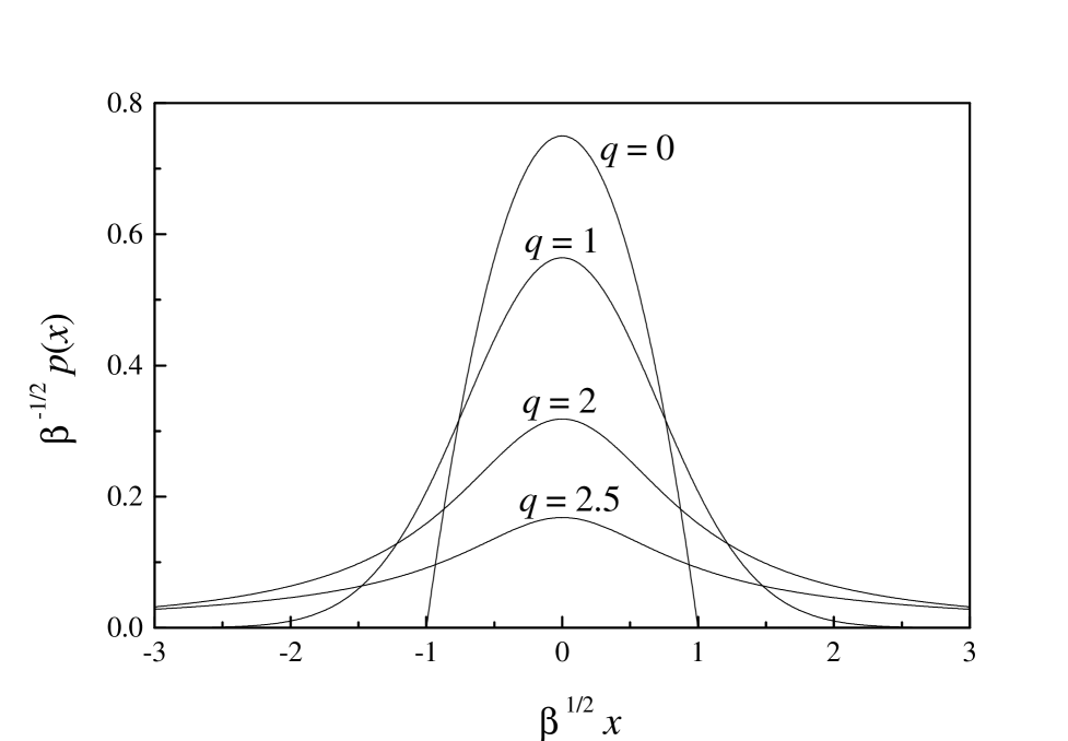
FIG. 3.: Jump probability distribution derived from Tsallis statistics, for some values of the Tsallis exponent $q$. For $q=1$ the standard Gaussian is obtained. Note the cut-off for $q<1$, and the long-tailed power-law distributions for $q>1$.

Regarding anomalous diffusion, thus, it is clear that the case $q<1$ is irrelevant. In fact, for such values of the Tsallis exponent $p(x)$ exhibits a cut-off at $|x|=1/\sqrt{\beta(1-q)}$, and vanishes for larger $|x|$, as shown by Eq. (38). This implies at once that the mean square displacement associated with $p(x)$ is finite and the resulting random walk corresponds to normal diffusion. The attention is consequently focused in the following on the case $1<q<3$, Eq. (37). In this case, the mean square displacement is

$$\langle x^{2}\rangle=\left\{\begin{array}[]{ll}[\beta(5-3q)]^{-1}&\mbox{if $q<5/3$,}\\ \\ \infty&\mbox{if $q\geq 5/3$}.\end{array}\right.$$ (40)

Therefore, for $1<q<5/3\approx 1.67$ the mean square displacement is still finite, and the random walk corresponds to normal diffusion. On the other hand, anomalous superdiffusion is obtained for $5/3\leq q<3$.

It is interesting to calculate now the $q$-expectation value of $x^{2}$ which, in the frame of Tsallis statistics, replaces –as an average quantity– the mean square displacement of the standard formulation. According to the constraint (34) imposed to $p(x)$ in the maximization of entropy, this $q$-expectation value should be finite. In fact,

$$\langle x^{2}\rangle_{q}=\frac{1}{2\beta}\left[\sqrt{\frac{(q-1)}{2\pi}}\frac{\Gamma\left(\frac{1}{q-1}\right)}{\Gamma\left(\frac{1}{q-1}-\frac{1}{2}\right)}\right]^{2(q-1)/(3-q)},$$ (41)

for $1<q<3$. The fact that, in contrast with the mean square displacement, $\langle x^{2}\rangle_{q}$ is finite, seems to indicate that the constraint (34) is a natural one in the frame of anomalous-diffusion random walks [25]. Note moreover that Eq. (41) along with (34) gives the connection between the Lagrange multiplier $\beta$ and the characteristic length $\sigma$,

$$\beta\propto\sigma^{-2}.$$ (42)

Equations (37) and (38) make clear that, as stated above, the maximization of entropy within Tsallis’ formalism does not lead to Lévy distributions for the jump probability. Rather, a plain power-law function of the jump length $x$ is obtained. Lévy distributions are however reobtained when considering the temporal evolution of the random walk generated by $p(x)$. In fact, the displacement $r$ of the walker after $t$ time steps is given by the sum of the successive jumps. By virtue of the generalized central limit theorem [18, 19] discussed in Section II B the probability distribution $P(r,t)$ is thus given, for large $t$ and $\gamma<2$ (i.e. $q\geq 5/3$), by a stable Lévy distribution with Lévy exponent $\gamma$. For $\gamma>2$, on the other hand, the usual form of the central limit theorem holds and the total displacement distribution is a Gaussian. The dynamic exponent $z$ of the random walk –which coincides with $\gamma$ for $\gamma<2$ (see Section II B)– is then

$$z=\left\{\begin{array}[]{ll}2&\mbox{if $q<5/3$,}\\ \\ (3-q)/(q-1)&\mbox{if $q\geq 5/3$}.\end{array}\right.$$ (43)

This connection between the dynamic exponent and the Tsallis exponent $q$ –which is illustrated by the curve $d=1$ in Figure 4– constitutes indeed the main result of the description of anomalous diffusion in the frame of the Tsallis’ formulation. It shows that a close relation exists between the properties of a Lévy-flight process and the non-extensiveness of the involved statistics. As far as the underlying statistical frame differs from Boltzmann-Gibbs’, the maximum-entropy formalism produces a random walk which models superdiffusion as a Lévy flight.

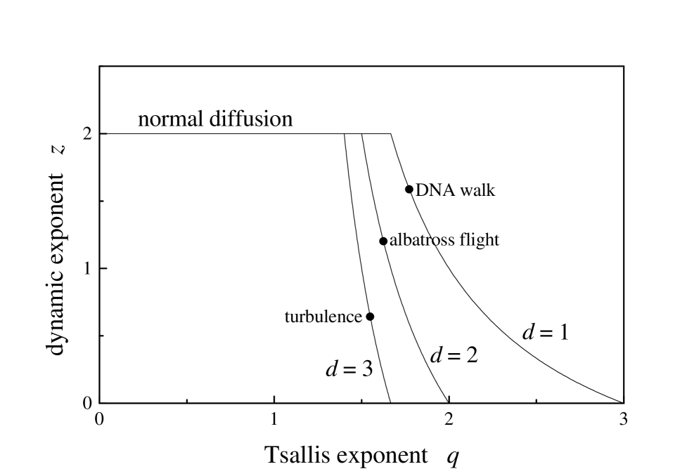
FIG. 4.: The diffusion dynamic exponent $z$ as a function of the Tsallis exponent $q$, for different spatial dimensions. The dots stand for some of the instances of anomalous diffusion discussed in Section II A.

As in the case of the jump distribution, the total mean square displacement $\langle r^{2}\rangle$ associated with Lévy flights diverges. On the other hand, the $q$-expectation value of $r^{2}$ is well defined for all relevant $q$ ($1<q<3$), cf. Eq. (41). This can be calculated taking into account the scaling properties of $P(r,t)$, Eq. (21), and reads

$$\langle r^{2}\rangle_{q}=\left\{\begin{array}[]{ll}D(q)\beta^{-1}t^{(3-q)/2}&\mbox{if $q<5/3$,}\\ \\ D(q)\beta^{-1}t^{q-1}&\mbox{if $q\geq 5/3$}.\end{array}\right.$$ (44)

The proportionality factor $D(q)$ depends on $q$ only. Interpreting now the Lagrange multiplier $\beta$ as the inverse of the temperature –as prescribed in the frame of Tsallis thermodynamics [27]– the above equation can be seen as a generalization of the Einstein relation (5) [30]. Equations (4) and (5) imply in fact that $\langle r^{2}\rangle\propto\beta^{-1}t$ for normal diffusion, and Eq. (44) is the extension of this result to Tsallis statistics. Again, the fact that $\langle r^{2}\rangle_{q}$ is finite for Lévy flights suggests that Tsallis’ formalism provides a natural frame for the statistical description of such kind of anomalous diffusion.

Though the algebra is more involved than above, anomalous diffusion in more than one dimension can be straightforwardly treated in the frame of Tsallis statistics, and the main conclusions are qualitatively the same as for the one-dimensional case. Maximazing the entropy given in (33) in the $d$-dimensional space produces formally the same jump distribution as in (35), where the partition function has however to be calculated as a $d$-dimensional integral. The jump probability can be normalized if

$$q<\frac{2+d}{d},$$ (45)

and the associated mean square displacement is finite if

$$q<\frac{4+d}{2+d}.$$ (46)

Below this value, thus, the random walk generated by the jump probability models normal diffusion, whereas for $(4+d)/(2+d)<q<(2+d)/2$ the walker performs superdiffusion. In Figure 5 these different regimes are identified in a phase diagram. The connection between the dynamic exponent and the Tsallis exponent reads now

$$z=\left\{\begin{array}[]{ll}2&\mbox{if $q<(4+d)/(2+d)$,}\\ \\ 2/(q-1)-d&\mbox{if $(4+d)/(2+d)<q<(2+d)/d$}.\end{array}\right.$$ (47)

This connection is represented graphically in Figure 4.

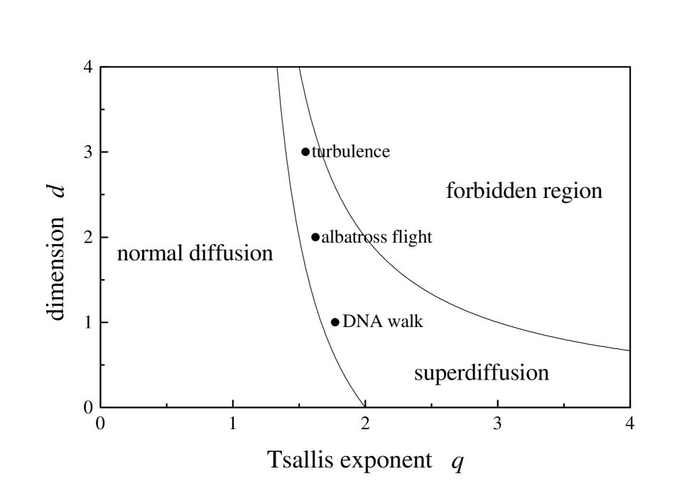
FIG. 5.: Phase diagram in the ($q,d$)-plane, displaying the zones of normal and anomalous diffusion, and the forbidden region where the jump probability distribution cannot be normalized. The dots stand for some of the instances of anomalous diffusion discussed in Section II A.

IV Nonlinear diffusion and Tsallis statistics

The diffusion equation,

$$\frac{\partial P}{\partial t}=D\nabla^{2}_{\bf r}P,$$ (48)

which governs the evolution of the probability $P({\bf r},t)\ d{\bf r}$ of finding a Brownian particle in a neighborhood $d{\bf r}$ of point $\bf r$ at time $t$, can be generalized to take into account additional mechanisms acting on both the microscopic dynamics of the particle and the mesoscopic dynamics of an ensemble of such particles. A rather straightforward generalization introduces for instance the effect of an external force field, ${\bf F}({\bf r},t)$, acting on each particle [3, 31]. This force field enters the diffusion equation as a drift term, namely,

$$\frac{\partial P}{\partial t}=-\nabla_{\bf r}\cdot({\bf F}P)+D\nabla^{2}_{\bf r}P.$$ (49)

This equation, which combines the effect of probability drift –due to the force– and of probability spreading –due to diffusion– can be seen to govern a huge class of random processes, in a generic space of states $\bf r$ [3, 31]. It is generally refered to as the Fokker-Planck equation.

Further generalizations, mainly justified on a phenomenological basis, have lead to propose a nonlinear version of the Fokker-Planck equation [32], namely,

$$\frac{\partial P^{\mu}}{\partial t}=-\nabla_{\bf r}\cdot({\bf F}P^{\mu})+D\nabla^{2}_{\bf r}P^{\nu},$$ (50)

where $\mu>0$ and $\nu$ are suitable real constants. Without loosing generality, one can fix $\mu=1$, by changing $P^{\mu}\to P$ and $\nu/\mu\to\nu$. In such case, Eq. (50) can be phenomenologically interpreted as a Fokker-Planck equation where, if $\nu\neq 1$, the diffusion coefficent depends on the probability $P({\bf r},t)$. This density-dependent diffusivity represents nonlinear effects arising, for instance, from interaction between the diffusing particles. Such kind of nonlinearities have been observed in several real processes, such as transport in porous media ($\nu\geq 2$) [33], surface growth ($\nu=3$) [34], liquid film spreading under gravity ($\nu=4$) [35], and Marshak radiative heat transfer ($\nu=7$) [36], among others [37].

The Fokker-Planck equation (49) is linear. This implies that for many forms of the force field ${\bf F}({\bf r},t)$ the general exact solution can be found analytically. Moreover, even if analytical solutions are not available or difficult to obtain, very efficient computational methods can be implemented to obtain numerical solutions. In contrast, exact solutions to the nonlinear equation (50) are particularly scarce [38, 39], and numerical methods are typically subject to instabilities when dealing with nonlinear problems. It is therefore of great interest to verify that, as shown in the following, Tsallis’ formalism provides a method to obtain special solutions to Eq. (50) for general $\mu$ and $\nu$, at least, in its one dimensional version and for some special forms of the drift force. This problem has recently been treated by Tsallis himself [40] and, in an alternate form, by Compte and Jou [41].

Consider then the one dimensional version of Eq. (50) for the probability density $P(x,t)$,

$$\frac{\partial P^{\mu}}{\partial t}=-\frac{\partial}{\partial x}[F(x)P^{\mu}]+D\frac{\partial^{2}P^{\nu}}{\partial x^{2}},$$ (51)

with $x\equiv r$, and with $F(x)=k_{1}-xk_{2}$. This time-independent, linear form of the drift force corresponds, in general, to a quadratic potential –i.e. an Ornstein-Uhlenbeck random process [3]– whereas it reduces to a linear potential –namely, a constant force– for $k_{2}=0$. For $\mu=\nu=1$, this equation can be straightforwardly solved, for instance, by Fourier-Laplace transforming. A special solution is

$$P(x,t)=\frac{1}{{\cal Z}(t)}\exp\left\{\beta(t)[x-\bar{x}(t)]^{2}\right\},$$ (52)

where

$$\frac{\beta(t)}{\beta(0)}=\left[\frac{{\cal Z}(0)}{{\cal Z}(t)}\right]^{2}=\left[(1-\Delta)\exp(-2k_{2}t)+\Delta\right]^{-1}$$ (53)

with $\Delta=2D\beta(0)/k_{2}$, and

$$\bar{x}(t)=\kappa+[\bar{x}(0)-\kappa]\exp(-k_{2}t)$$ (54)

with $\kappa=k_{1}/k_{2}$. This particular solution has the important property that, for $t\to 0$ and $\beta(0)\to\infty$, it reduces to a delta-like distribution, $P(x,0)=\delta[x-\bar{x}(0)]$. Since Eq. (51) is linear for $\mu=\nu=1$, and delta distributions can be used as a base for the space of initial conditions $P(x,0)$, a suitable linear combination of functions of the form (52) provides the solution to the linear equation for any initial condition in that space. In this sense, (52) gives the general solution to the linear Fokker-Planck equation with the above prescribed drift force.

Focus now the attention on the functional form of the particular solution to the linear problem given in Eq. (52). As a function of $x$, $P(x,t)$ is a Gaussian, essentially of the same type as (28). The differences are, firstly, that the spatial coordinate $x$ is shifted by an amount $\bar{x}(t)$. The Gaussian is therefore centered around a position which depends on time. Secondly, the width of the Gaussian, which is proportional to $\beta^{-1/2}$, depends also on time. Since the solution (52) preserves normalization, the normalization factor ${\cal Z}^{-1}$ is time-dependent.

The Gaussian profile of $P(x,t)$ in Eq. (52) suggests that this solution can be formally derived from a suitably extended maximum-entropy formalism, in its standard Boltzmann-Gibbs version. In fact, it can be shown [40] that such form of $P(x,t)$ derives from the maximization of

$$S[P]=\int_{-\infty}^{+\infty}P(x,t)\ln P(x,t)\ dx,$$ (55)

with the extended constrains

$$\int_{-\infty}^{+\infty}P(x,t)\ dx=1,$$ (56)

$$\int_{-\infty}^{+\infty}[x-\bar{x}(t)]P(x,t)\ dx=0,$$ (57)

and

$$\int_{-\infty}^{+\infty}[x-\bar{x}(t)]^{2}P(x,t)\ dx=\frac{1}{2\beta(t)},$$ (58)

for arbitrary $\bar{x}(t)$ and $\beta(t)$. The special forms of these functions that make the probability distribution satisfy the linear Fokker-Planck equation can be obtained by simply replacing $P(x,t)$ in the equation.

It should be by now clear that one is immediately interested at which solutions are obtained if, instead of the standard maximization principle, the Tsallis’ formalism is used. Namely, take the generalized entropy

$$S_{q}[P]=-\frac{1}{1-q}\left\{1-\int_{-\infty}^{+\infty}P(x,t)^{q}dx\right\},$$ (59)

and maximize it with respect to $P(x,t)$ imposing the generalized constrains

$$\int_{-\infty}^{+\infty}[x-\bar{x}(t)]P(x,t)^{q}dx=0,$$ (60)

and

$$\int_{-\infty}^{+\infty}[x-\bar{x}(t)]^{2}P(x,t)^{q}dx=\frac{1}{2\beta(t)}.$$ (61)

This produces [40]

$$P(x,t)=\frac{1}{{\cal Z}_{q}(t)}\left\{1-\beta(t)(1-q)[x-\bar{x}(t)]^{2}\right\}^{1/(1-q)},$$ (62)

to be compared with Eq. (35). Remarkably enough, this form of $P(x,t)$ turns out to be a solution to the one-dimensional nonlinear Fokker-Planck equation for the linear drift force if

$$q=1+\mu-\nu,$$ (63)

and

$$\frac{\beta(t)}{\beta(0)}=\left[\frac{{\cal Z}_{q}(0)}{{\cal Z}_{q}(t)}\right]^{2\mu}.$$ (64)

As for Lévy-flight anomalous diffusion, $P(x,t)$ can be normalized only if $q<3$. This defines a forbidden region for $\mu>2+\nu$ (Fig. 8).

The function ${\cal Z}_{q}(t)$ is explicitely given by

$${\cal Z}_{q}(t)={\cal Z}_{q}(0)\left[(1-\Delta_{q})\exp(-t/\tau)+\Delta_{q}\right]^{1/(\mu+\nu)},$$ (65)

with

$$\Delta_{q}=\frac{2\nu D\beta(0){\cal Z}_{q}(0)^{\mu-\nu}}{k_{2}},$$ (66)

and $\tau=\mu/k_{2}(\mu+\nu)$. The function $\bar{x}(t)$ is the same as for the linear case, Eq. (54). Note that the normalization constraint, Eq. (56), has not been imposed in the maximization of $S_{q}[P]$. In fact, the preservation of the norm of $P(x,t)$ is now not compatible with the other two constraints. Rather, it turns out that the integral of the probability density over the whole space varies with time according to

$$\int_{-\infty}^{+\infty}P(x,t)\ dx=\left[\frac{{\cal Z}_{q}(t)}{{\cal Z}_{q}(0)}\right]^{\mu-1}\int_{-\infty}^{+\infty}P(x,0)\ dx.$$ (67)

This implies that the norm is conserved for all times only if $\mu=1$, or if $\Delta_{q}=1$ –when ${\cal Z}_{q}$ does not depend on time. If $\Delta_{q}>1$ the norm monotonically increases for $\mu>1$ and decreases for $\mu<1$. If $\Delta_{q}<1$, on the other hand, the opposite behavior is observed. Moreover, for $\nu<0$ the norm diverges or vanishes at a finite time. Figure 6 illustrates these different regimes for $\nu=1$ and some values of $\mu$.

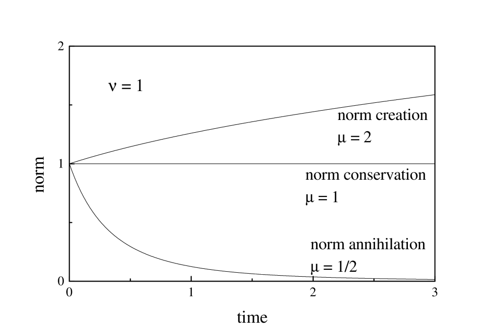
FIG. 6.: Evolution of the norm in the solutions to the nonlinear Fokker-Planck equation for $\nu=1$ and some values of $\mu$. These curves correspond to $\Delta_{q}>1$.

The case of constant force, $k_{2}=0$, can be analyzed as the suitable limit of the above solution for $k_{2}\to 0$. In particular, taking $\exp(-t/\tau)\approx 1-t/\tau$ in Eq. (65) it is found that

$${\cal Z}_{q}(t)={\cal Z}_{q}(0)\left[1+2\frac{\nu(\nu+\mu)}{\mu}D\beta(0){\cal Z}_{q}(0)^{\mu-\nu}t\right]^{1/(\mu+\nu)}.$$ (68)

In this limit, the width of the distribution –which is proportional to $\beta^{-1/2}$– exhibits a well-defined power-law dependence on time. In fact, according to Eq. (64), $\beta(t)^{-1/2}\propto t^{\mu/(\nu+\mu)}$. This makes possible to assign a dynamic exponent to this kind of diffusion, given by

$$z=1+\frac{\nu}{\mu}.$$ (69)

Whereas, as expected, the case $\mu=\nu=1$ corresponds thus to normal diffusion, $\nu/\mu>1$ corresponds to subdiffusion and $\nu/\mu<1$ corresponds to superdiffusion. Note that if $\nu/\mu<-1$, $z<0$ and the distribution width decreases with time. This seemingly unphysical situation [40] can however be associated with a kind of “negative diffusivity”, which has been observed in some real nonequilibrium self-organizing systems [38]. Figure 7 shows the evolution of the distribution width for $\mu=1$ and various values of $\nu$. The phase diagram of Figure 8 summarizes the various regimes obtained in different regions of the ($\nu,\mu$)-plane.

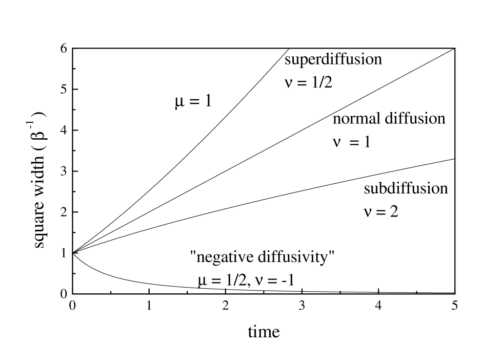
FIG. 7.: Evolution of the width in the solutions to the nonlinear Fokker-Planck equation for $\mu=1$ and some values of $\nu$. For the case of “negative diffusivity,” $\mu=1/2$.

Equation (63) makes evident that the non-extensivity inherent to Tsallis statistics is related, in the frame of its application to the resolution of the nonlinear Fokker-Planck equation (51), to the nonlinearity of the equation itself. This nonlinearity translates, at the level of the solutions, into anomalous properties of the involved transport processes. Thus, a clear connection between anomalous diffusion and the non-extensivity of the underlying statistics arises again. It is important to point out that, in contrast with Eq. (52), the solutions (62) to the nonlinear Fokker-Planck equation derived from Tsallis’ formalism cannot be combined to give a general solution. In fact, due to the nonlinearity of Eq. (51), no superposition principle holds, and (62) are particular solutions for special initial conditions only. Nevertheless, the straightforward way in which these solutions have appeared as an extension of the linear case along the lines of Tsallis’ generalization, reinforces strongly the close relation between Tsallis’ formalism an anomalous diffusion.

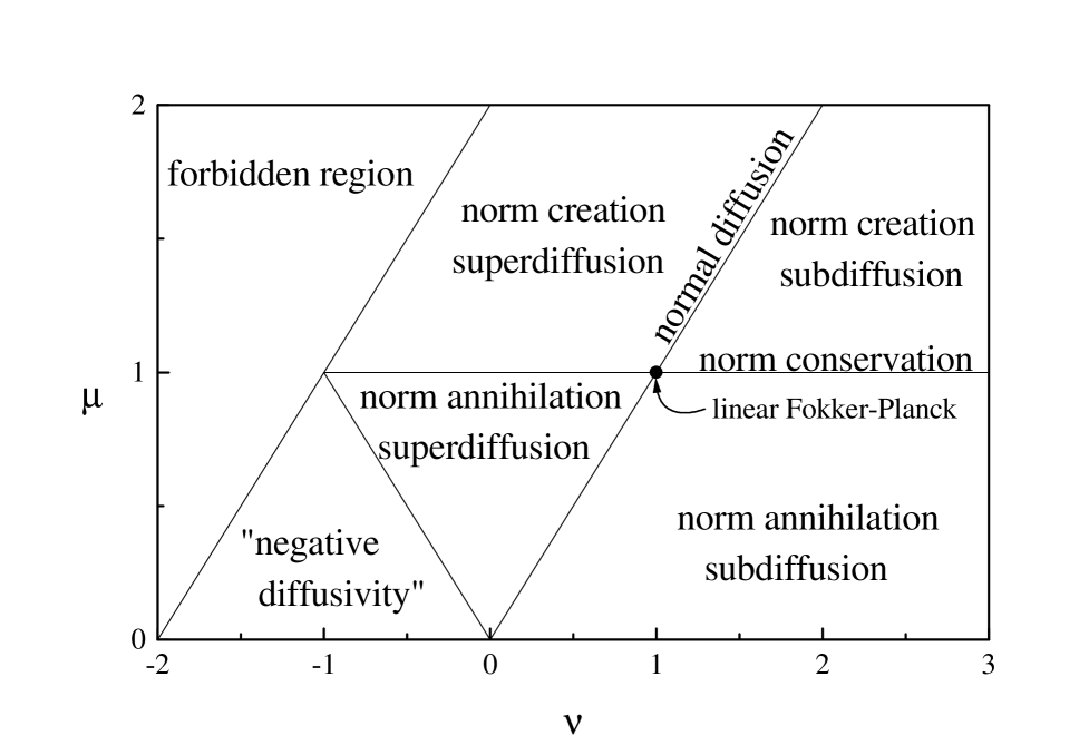
FIG. 8.: Phase diagram in the ($\nu,\mu$)-plane, displaying the different regimes of anomalous diffusion and norm evolution in the solutions to the nonlinear Fokker-Planck equation. In the forbidden region the probability distribution cannot be normalized.

V Conclusion

Though normal diffusion is ubiquitous in Nature, a large –and still growing– class of real systems is driven by a different kind of transport processes, namely, by anomalous diffusion. In view of the current importance of many of these systems –which range from turbulent flows, to disordered media and chaotic dynamics, to flight patterns in birds– it is of high interest having at hand a formulation able to place anomalous diffusion in a statistical-thermodynamical frame, generalizing thus Einstein’s theory for normal diffusion. However, within Boltzmann-Gibbs statistics “the wonderfull world of clusters and intermittencies and bursts that is associated with Lévy distributions would be hidden from us if we depended on a maximum entropy formalism that employed simple traditional auxiliary conditions” [24]. It has been here shown that, instead, Tsallis generalized statistics is a strong candidate to succesfully yield such a formulation.

Tsallis statistics provides a natural frame for the mathematical foundations of anomalous diffusion in two forms. In the first place, jump distributions of random-walk models for Lévy-like superdiffusion can be straightforwardly derived from a maximum-entropy principle within the generalized theory. In fact, such distributions exhibit power-law long tails, which are an essential feature in the results of the theory. At once, Tsallis statistics furnishes an elegant explanation for the appearence of Lévy distributions in other natural phenomena, as the result of the superposition of random variables with long-tailed distributions. In the second place, the functional form of the distributions resulting from Tsallis’ formalism successfully suggests the solution to the nonlinear Fokker-Planck equation, which describes both subdiffusion and superdiffusion.

In order to widen the applications of Tsallis’ theory to the statistical foundations of anomalous diffusion, further research should focus on some problems that still wait to be treated in the frame of the generalized statistics. For instance, it would be important to extend the derivation of random-walk models of anomalous diffusion to the case of subdiffusion. As explained in Section II, this requires introducing suitable waiting-time densities. Since power-law functions can fulfill this role, Tsallis statistics is again a natural stating point to derive such densities. Another extension would regard diffusion processes on fractals. In fact, Lévy-like diffusion anomalies are the consequence of mechanisms driving the dynamics of the diffusing particles. An alternative formulation, which is relevant to many applications, takes into account that such anomalies originate rather in the complex geometry of the medium where particles diffuse. The connection between fractal geometry and Tsallis statistics has been identified early, and it can thus be expected that diffusion on fractal substrates finds a satisfactory statistical-mechanical frame in such theory. Finally, it would be interesting to descend a level further in the dynamical bases of anomalous diffusion, and try to apply Tsallis’ formalism to the formulation of deterministic mechanical approaches to this kind of transport.

As a final remark it is worth mentioning that, very recently, Tsallis’ formalism has been improved by redefining the normalization of $q$-expectation values [42]. This has solved, in a single step, two main drawbacks of the theory. In fact, in its original formulation, Tsallis statistical mechanics is not invariant under energy shifts, and the $q$-expectation value of a constant depends on the state of the system under study. Although the correction to the theory does not involve important changes in the qualitative results, it represents a major improvement from a formal viewpoint. Here, Tsallis statistics has been applied to anomalous diffusion in its original form. A relevant step forward would be to reanalyze this process in the frame of the corrected theory.

REFERENCES

- [1] A. Einstein, Ann. Phys. 17, 549 (1905).
- [2] E.W. Montroll and B.J. West, in Fluctuation Phenomena, E.W. Montroll and J.L. Lebowitz, eds. (Elsevier, Amsterdam, 1979) p. 61.
- [3] N.G. van Kampen, Stochastic Processes in Physics and Chemistry (North-Holland, Amsterdam, 1992).
- [4] R. Kubo, Statistical Mechanics (North-Holland, Amsterdam, 1988).
- [5] J.-P. Bouchaud and A. Georges, Phys. Rep. 195, 127 (1990).
- [6] J. Bernasconi et al., Phys. Rev. Lett. 42, 819 (1979).
- [7] J. Machta, J. Phys. A 18, L531 (1985).
- [8] L.F. Richardson, Proc. Roy. Soc. London, Ser. A 110, 709 (1926).
- [9] B.B. Mandelbrot, J. Fluid Mech. 62, 331 (1974).
- [10] R.A. Antonia, N. Phan-Thien, and B.R. Satyoparakash, Phys. Fluids 24, 554 (1981).
- [11] M.F. Shlesinger, B.J. West, and J. Klafter, Phys. Rev. Lett 58, 1100 (1987).
- [12] G.M. Zaslavsky, R.Z. Sagdeev, and A.A. Chernikov, Sov. Phys. JETP 67, 270 (1988); A.A. Chernikov et al., Phys. Lett. A 144, 127 (1990).
- [13] M.F. Shlesinger, G.M. Zaslavski, and J. Klafter, Nature 363, 31 (1993).
- [14] E.R. Weeks et al., in Lévy Flights and Related Topics in Physics, M.F. Shlesinger, G.M. Zaslavsky, and U. Frisch, eds. (Springer, Berlin, 1995) p. 51.
- [15] C.-K. Peng et al., Nature 356, 168 (1992).
- [16] H.E. Stanley et al., in Lévy Flights and Related Topics in Physics, M.F. Shlesinger, G.M. Zaslavsky, and U. Frisch, eds. (Springer, Berlin, 1995) p. 331.
- [17] G.M. Viswanathan et al., Nature 381, 413 (1996).
- [18] P. Lévy, Théorie de l’addition des variables aléatoires (Gauthier-Villars, Paris, 1937).
- [19] A. Araújo and E. Giné, The Central Limit Theorem for Real and Banach Valued Random Variables (Wiley, New York, 1980).
- [20] B.D. Hughes, M.F. Shlesinger, and E.W. Montroll, Proc. Acad. Sci. USA 78, 3287 (1981).
- [21] A. Compte, Phys. Rev. E 53, 4191 (1996).
- [22] H.C. Fogedby, Phys. Rev. E 50, 1657 (1993).
- [23] C. Tsallis, A.M.C. Souza, and R. Maynard, in Lévy Flights and Related Topics in Physics, M.F. Shlesinger, G.M. Zaslavsky, and U. Frisch, eds. (Springer, Berlin, 1995) p. 269.
- [24] E.W. Montroll and M.F. Shlesinger, J. Stat. Phys. 32, 209 (1983).
- [25] P.A. Alemany and D.H. Zanette, Phys. Rev. E 49, 956 (1994).
- [26] C. Tsallis, J. Stat. Phys. 52, 479 (1988).
- [27] E.M.F. Curado and C. Tsallis, J. Phys. A 24, L69 (1991) [corrigenda 24, 3187 (1991); 25, 1019 (1992)].
- [28] C. Tsallis, Chaos, Solitons & Fractals 6, 539 (1995).
- [29] C. Tsallis et al., Phys. Rev. Lett. 75, 3589 (1995).
- [30] D.H. Zanette and P.A. Alemany, Phys. Rev. Lett. 75, 366 (1995).
- [31] H.S. Wio, An Introduction to Stochastic Processes and Nonequilibrium Statistical Physics (World Scientific, Singapore, 1994).
- [32] A formal derivation of the nonlinear Fokker-Planck equation from a Langevin equation within the frame of Tsallis statistics has recently been proposed in L. Borland, Phys. Rev. E 57, 6634 (1998).
- [33] M. Muskat, The Flow of Homogeneous Fluids Through Porous Media (McGraw-Hill, New York, 1937); P.Y. Polubarinova-Kochina, Theory of Ground Water Movement (Princeton University Press, Princeton, 1962).
- [34] H. Spohn, J. Phys. (France) I 3, 69 (1993).
- [35] J. Buckmaster, J. Fluid Mech. 81, 735 (1977).
- [36] E.W. Larsen and G.C. Pomraning, SIAM J. Appl. Math. 39, 201 (1980).
- [37] W.L. Kath, Physica D 12, 375 (1984).
- [38] J.D. Murray, Mathematical Biology (Springer, Berlin, 1989).
- [39] J.R. King, J. Phys. A 23, 3681 (1990); D.H. Zanette, J. Phys. A 26, 5339 (1993).
- [40] C. Tsallis and D.J. Bukman, Phys. Rev. E 54, R2197 (1996).
- [41] A. Compte and D. Jou, J. Phys. A 29, 4321 (1996).
- [42] C. Tsallis, R.S. Mendes and A.R. Plastino, The role of constraints within generalized nonextensive statistics, Physica A (1998, in press).