Modeling nonlinearity and hysteresis due to critical-state flux penetration in hard superconductors

Abstract

The nonlinear surface impedance of a thin superconducting strip carrying a microwave current has been calculated numerically from first principles based upon flux penetration due to a current-induced critical state. The calculations approach analytic results in the appropriate limit. The technique is useful for design of passive superconducting microwave circuits.

I Introduction

Since its discovery, the new breed of oxide superconductors with transition temperatures above the boiling point of nitrogen have shown great potential as a replacement for metals for passive microwave structures owing to their very low surface resistance[1, 2, 3]. However, a key feature of the HTSC is the inherently nonlinear response at microwave frequencies, which is present over a wide range of input powers. This nonlinear responses also poses a major challenge for numerical device design using these materials. Most existing computer aided design software do not take into account the inherent nonlinearity of superconductors. The few analytical models that do exist[4] are valid only for highly idealized geometries and need to be incorporated into practical device design.

There are several physical models of nonlinear surface resistance, each valid in a different regime of temperature and microwave power[5]. The most pursued ones are pinning induced critical state[4, 6, 7], transport current induced self-heating [8], and depairing [8]. The current-driven critical state model [4] has proven to be particularly useful not only because it fits experimental measurement of $R_{S}$ very accurately over a wide range of temperature and power levels [9], but also because its usefulness extends to modeling hysteretic losses in superconducting transmission lines.

The (field-induced) critical state model was first proposed by Bean[10] to explain the unusual magnetization behavior of hard superconductors and was first solved for the geometry of a semi-infinite slab where the field was applied parallel to its face. The geometry where the field is applied perpendicular to a thin strip was solved relatively recently by several groups and the field and current distribution[11, 12] and the surface impedance from hysteretic loss[4] was obtained analytically.

Though very elegant, the analytic results were restricted to certain “ideal” geometries only where symmetry could be used to simplify the problems. However, these idealizations are not always satisfied in real world applications of superconducting strips in microwave circuits. In the wake of the fact that the model does describe experimental data accurately [9], it is imperative to be able to implement a numerical paradigm without the constraints of the idealized geometry required by the analytic approach.

In this paper, we demonstrate a numerical approach to incorporate the nonlinear response of superconducting materials using assumptions equivalent to those of the current induced critical state.

II The Critical State Model

Let us consider a stripline with the ground plane far away from the center conductor so that it carries a negligible current and hence does not effect the magnetic field distribution inside the center conductor. It has been shown in literature that such an assumption is reasonable[13] (We will discuss the effects of ground planes somewhere else.) The geometry of the center conductor and our choice of axes is shown in of Fig. 1.

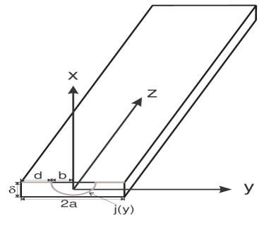
Figure 1: The geometry of the problem. The strip is centered around $x=y=0$.

Starting from the most generic physical assumptions that retain the essential ideas of critical states:

1. $|{\bf j}({\bf r})|\leq j_{c}$ where ${\bf j}$ is the current density.

2. The magnetic induction ${\bf B}(x,y)=0$ for $|y|\leq b\leq a$

The first assumption highlights the fact that flux lines are pinned until the Lorenz force on them exceeds a certain critical value. The second assumption follows from the fact that the vortices start penetrating from the edges. Hence for any given current there would be a flux free region in the center of the strip. Note that the depinning critical current is at least an order of magnitude smaller than the depairing critical current where superconductivity would be quenched by the self field.

In the following we show that for a strip with finite thickness, this model can be solved numerically and that it leads to unique field and current distribution within the strip. We further show that $(1)$ and $(2)$ leads to hysteresis irrespective of the geometry and study the hysteresis laws for the specific strip geometry under consideration.

III Computational Details

A semi-numerical approach was used to determine a current distribution which satisfies the two assumptions presented above. Assuming an uniform current distribution along the x-direction one can show that

$${\bf B}(x=0,y)=\frac{\mu_{0}}{\pi}\int_{-a}^{a}{\bf j}(y^{\prime})\tan^{-1}[\frac{\delta}{2(y-y^{\prime})}]dy^{\prime}$$ (1)

The above analytical expression for $B(x=0,y)$ in Eq(1) was used to save computational time.

In the model which requires that ${\bf j}(y:b\leq|y|\leq a)\equiv J_{c}$ and $B(x=0,|y|\leq b<a)=0$, one needs to solve for the current distribution in the field free region $|y|\leq b<a$

$$\int_{-a}^{a}{\bf j}(y^{\prime})\tan^{-1}[\frac{\delta}{2(y-y^{\prime})}]dy^{\prime}=0\;{\rm for\;}|y|\leq b<a$$ (2)

Numerical solutions of integral equations such as eq(2) are rather complicated. We found a simpler iterative approach to find the current density in the field free region of the superconducting strip. Here we give a brief description of the algorithm that was used.

Suppose that the thickness of the strip is infinite ($\delta\rightarrow\infty$.). Then for any given initial current distribution ${\bf j}(y)$, a field free region $B(|$ $y|\leq b)\equiv 0$ can be obtained by replacing the current density in that region by

$$j(|y|<b)\Rightarrow j(|y|)+\frac{\partial}{\partial y}B_{x}$$ (3)

Also note that the magnetic field strength on the line $x=0$ for a slab ($\delta\rightarrow\infty$.) is mostly effected by the current on and around the line $x=0$. Therefore, for the case of a finite $\delta$, the transformation in eq(3) will bring the field strength in the region $|y|<b$ a little closer to zero. Hence an iterative implementation of the above transformation of $J(y)$ in eq(3) will finally converge bringing the magnetic field strength in the region $|y|<b$ to zero, irrespective of the size of $\delta$.

In a nutshell, we start with a flat current distribution, ${\bf j}(y)=j_{c}$ in an one dimensional grid of size $4000$ and we iteratively make ${\bf B}(x=0,|y|<b)$ vanish by replacing the current density by $j_{y}^{n+1}\Rightarrow j_{y}^{n}+\left(B_{y+1}^{n}-B_{y}^{n}\right)/\Delta y$.

IV Results

IV-A Penetration Law

We calculate the flux penetration depth $d/a$ for a strip of aspect ratio of 1% as a function of the applied current. In Fig.2 we display $(1-d/a)=b/a$ as a function of the applied current $y/a$ and compare that with the analytical results for a strip of zero thickness[12]. Fig.3 and Fig. 4 shows the corresponding current and field distributions. One can see from Fig.2 and Fig.3 that the penetration law get’s more linear and the current density in the field free region decreases as we go from zero thickness to a finite thickness. These results are expected since, in the limit $\delta\rightarrow\infty$ we expect a linear penetration law and $J(x=0,|y|\leq b<a)=0$. These results can then determine the current critical states and the corresponding magnetic field distribution for AC currents with a peak current of $I_{0}$.

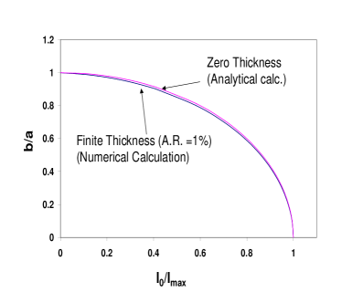
Figure 2: Penetration depth $b$ as a function of current $I/I_{\mbox{max}}$.

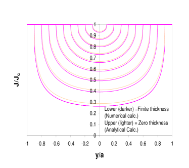
Figure 3: Current distribution $j/j_{c}$ across the strip for $b/a=0.1,0.2,\ldots,0.9$. The lower (solid) lines are numerical calculations and the upper (dashed) lines are analytic calculations.

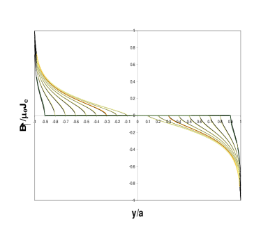
Figure 4: The magnetic field strength $B(x=0,y/a)$ across the strip for $I/I_{\rm max}=0.41,0.58,0.70,0.79,0.86,0.91,0.95,0.98,0.99$.

V Hysteresis

The hysteresis law can be derived by studying the current density distribution for an oscillating current over a full cycle. If the current density distribution for a total current $I$ is $j(y,I,j_{c}\rightarrow\infty)$ then in absence of pinning the current density will be $Nj(y,I,j_{c}\rightarrow\infty)$ for a total current of $NI$. In other words

$$j(y,NI,j_{c}\rightarrow\infty)=Nj(y,I,j_{c}\rightarrow\infty)$$ (4)

However, since $j(y)\leq j_{c}$ everywhere, the current density distribution depends on the total current. That is

$$j(y,NI,j_{c})\neq Nj(y,I,j_{c}).$$ (5)

When the current is reversed, after reaching the peak $I_{0}$, current density starts to decrease from the edges with an effective critical current density in the opposite direction of $2J_{c}$. This is because at the edges the current density is $j_{c}$ in the positive x-direction.

$$j_{c\downarrow}=2j_{c\uparrow}$$ (6)

Thus the hysteresis law on the downward cycle is given by[12]

$$j_{\downarrow}(y,I,j_{c})=j_{\mbox{max}}(y,I_{0},j_{c})-j_{\uparrow}(y,I_{0}-I,2j_{c})$$ (7)

Fig. 5 displays the magnetic field distribution when the input current is reduced from the maximum current $2J_{c}\delta a$ to $-2J_{c}\delta a$. As the decreases through $0$ one does not see any field free region inside the strip, that is there are locked in fields from field distribution when the total current was $2J_{c}\delta a$: something that is unique to hysteresis.

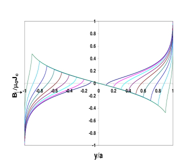
Figure 5: Magnetic field strength, $B(x=0,y/a)$, when $I$ is reduced from $I_{\mbox{max}}=2J_{c}\delta a$ to $-I_{\mbox{max}}$. This graph dispalys the origin of hysteresis. We plot $B$ across the strip for $I/I_{\rm max}=0.18,-0.17,-0.40,-0.58,-0.72,-0.82,-0.90,-0.96,-0.99$.

VI Surface Impedance

Assuming that the strip is excited with a current of amplitude $I_{0}$ and frequency $\omega_{0}$, the electric field $E(y,t)$ is be given by

$$E_{Z}(y,t)=\frac{d\ }{dt}\int_{0}^{a}dy^{\prime}\ B_{x}(y^{\prime},t)$$ (8)

and the energy lost in a half cycle is

$$U_{H.C.}=2\int_{0}^{a}dy\int_{-T/4}^{T/4}dt\;J(y,t)E(y,t)$$ (9)

Substituting eq(8) and integrating by parts we get

$$U_{H.C.} = 2\int_{0}^{a}dy\int_{-T/4}^{T/4}dt\;J_{c}\frac{d\ }{dt}\int_{b(I_{0})}^{a}dy^{\prime}\ B_{x}(y^{\prime},t)$$ (10)

$$= 4\mu_{0}J_{c}\int_{b(I_{0})}^{a}dy\int_{b(I_{0})}^{a}dy^{\prime}B_{x}(y^{\prime},t)$$ (11)

This definition of $U_{H.C.}$ was also used by Brandt in ref.[12]. This defines the surface resistance as

$$R_{s}=2\frac{4\mu_{0}J_{c}}{I_{0}^{2}T}\int_{b(I_{0})}^{a}dy\int_{b(I_{0})}^{a}dy^{\prime}B_{x}(y^{\prime},t)$$ (12)

Fig. 6 displays the surface resistance $R_{s}$ as a function of the peak current, $I_{0}$.

The surface reactance $X_{s}$ per unit length can be calculated using the average total electrostatic energy per unit length.

$$X_{s}=\frac{1}{\mu_{0}I_{0}^{2}T}\int_{0}^{T}\int B^{2}(x,y)d^{2}s_{xy}$$ (13)

We carry out the space integral until $B^{2}(x,y)$ falls down by $99\%$ of it’s peak value. Fig. 7, displays the surface reactance $X_{s}$ as a function of the peak current, $I_{0}$. Our results are close to the analytical results in ref.[4].

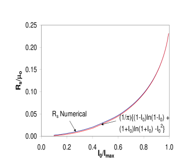
Figure 6: Surface resistance $R_{s}$ as a function of the current $I/I_{\mbox{max}}$.

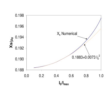
Figure 7: Surface reactance $X_{s}$ as a function of the current $I/I_{\mbox{max}}$.

VII Conclusion

A first principle numerical calculation on a strip of finite thickness using assumptions similar to the critical state model yields results that approach the analytic results in the appropriate limits $\left(\delta\rightarrow 0\right)$ but without the unrealistic idealizations of the later. Further a numerical approach gives one the flexibility of accommodating higher complexities like effects due to the ground planes and more accurate calculations of surface impedance and harmonics. This topic will be addressed in future work. This approach can be implemented into a computer aided design framework for the design of passive superconducting microwave components.

VIII Acknowledgments

This work is supported by NSF-9711910 and AFOSR.

References

- [1] Durga P. Choudhury and S. Sridhar, “Superconducting microwave technology,” in Wiley’s Encyclopedia of Electrical and Electronic Engineering, John Webster, Ed. John Wiley & Sons, New York, 1999.
- [2] M. J. Lancaster, Passive microwave device applications of high temperature superconductors, Cambridge University Press, New York, 1997.
- [3] Zhi-Yuan Shen, High-Temperature Superconducting Microwave Circuits, Artech House, Boston, 1994.
- [4] S. Sridhar, “Non-linear microwave impedance of superconductors and ac response of the critical state,” Appl. Phys. Lett., vol. 65, no. 8, pp. 1054–1056, August 1994.
- [5] M. A. Golosovsky, H. J. Snortland, and M. R. Beasley, “Nonlinear microwave properties of superconducting Nb microstrip resonators,” Phys. Rev. B, vol. 51, no. 10, pp. 6462–6469, March 1995.
- [6] J. McDonald, John R. Clem, and D. E. Oates, “Critical-state model for harmonic generation in a superconducting microwave resonator,” Phys. Rev. B, vol. 55, no. 17, pp. 11823–11831, May 1997.
- [7] J. McDonald, J. R. Clem, and D. E. Oates, “Critical-state model for intermodulation distortion in a superconducting microwave resonator,” J. Appl. Phys., vol. 83, no. 10, pp. 5307–5312, May 1998.
- [8] M. Golosovsky and M. Tsindlekht and H. Chayet and D. Davidov “Vortex depinning frequency in superconducting thin films — anisotropy and temperature dependence,” Phys. Rev. B, vol. 50, no. 1, pp. 470, Jul 1994.
- [9] Balam A. Willemsen, John S. Derov, José H. Silva, and S. Sridhar, “Nonlinear response of suspended high temperature superconducting thin film microwave resonators,” IEEE Trans. Appl. Supercond., vol. 5, no. 2, pp. 1753–1755, June 1995.
- [10] C. P. Bean, “Magnetization of hard superconductors,” Phys. Rev. Lett., vol. 8, pp. 250–253, 1962.
- [11] E. Zeldov, John R. Clem, M. M. McElfresh, and M. Darwin, “Magnetization and transport currents in thin superconducing films,” Phys. Rev. B, vol. 49, no. 14, pp. 9802–9822, April 1994.
- [12] Ernst Helmut Brandt and Mikhail Indenbom, “Type-II-superconductor strip with current in a perpendicular magnetic field,” Phys. Rev. B, vol. 48, pp. 12893–12906, 1993.
- [13] A. M. Campbell, “ ” IEEE Trans. Appl. Supercond., vol. 5, pp. 687, 1995.