Physics on the edge: contour dynamics, waves and solitons in the quantum Hall effect

Abstract

We present a theoretical study of the excitations on the edge of a two-dimensional electron system in a perpendicular magnetic field in terms of a contour dynamics formalism. In particular, we focus on edge excitations in the quantum Hall effect. Beyond the usual linear approximation, a non-linear analysis of the shape deformations of an incompressible droplet yields soliton solutions which correspond to shapes that propagate without distortion. A perturbative analysis is used and the results are compared to analogous systems, like vortex patches in ideal hydrodynamics. Under a local induction approximation we find that the contour dynamics is described by a non-linear partial differential equation for the curvature: the modified Korteweg-de Vries equation.

I Introduction

The theoretical description of many-body systems is often best realized in terms of collective modes, i.e. the familiar sound waves in solids or plasmons in charged systems. Collective modes become especially important when their energies are lower than competing single-particle excitations. Sometimes, however, both single-particle and collective modes in the bulk of a system are gapped or scarce and these systems are often referred to as “incompressible.” This incompressibility can be real or a convenient limit due to large differences in relevant length- or time-scales, as in the case of the macroscopic motion of a liquid. Under these conditions, one can usually focus our attention on the motion of the boundaries of the system, which will generally have softer modes, with frequencies much lower than those in the bulk (e.g. surface waves in a liquid droplet travel at speeds considerably slower than sound waves).

Concentrating on the motion of the boundary of the system has a considerable advantage: the reduction in the dimensionality of the problem often permits simpler analytical treatment, or a tremendous reduction in the effort needed to numerically solve or simulate the problem. Associated with this incompressibility, however, one usually finds microscopic conservation laws that translate into global constraints on the whole system, even when the microscopic dynamics is completely local (e.g. the volume of a liquid droplet is conserved). These global constraints enter the edge dynamics through Lagrange multipliers associated with the conserved quantities.[1] These conservation laws are often evident when the motion of the system is observed, and it is interesting to see how they are embedded in the dynamics of the boundary; that is, how these essential aspects of the problem are related to the laws of motion of the edges.

These shape deformations, and their dynamics, have played an important role in the understanding of numerous problems in diverse fields of physics. The incompressibility is reflected in the existence of a field which is piecewise constant, so that there is a sharp boundary between two or more distinct regions of space with different physical properties. This field can be of classical origin like the density of a liquid or the charge density of a plasma, or it can originate in the quantum mechanical properties of the system, like the magnetization of a type-II superconductor. There are various examples where these questions are relevant, such as waves on the surface of a liquid,[2, 3, 4] the motion of non-neutral plasmas,[5] low lying “rotation-vibration” modes of deformed nuclei,[6] the evolution of atmospheric plasma clouds,[7] pattern formation in ferromagnetic fluids,[8] vortex patches in ideal fluids,[9, 10, 11, 12] and two-dimensional electron systems (2DES) in strong magnetic fields.[13, 14]

The edges of a two-dimensional electron system (2DES), and in particular the edges of a quantum Hall (QH) liquid, present a unique opportunity to study the dynamics of shape deformations in a clean and controlled environment. The 2DES in the QH state is incompressible, so that the electron density is approximately piecewise constant, suggesting that a contour dynamics approach to studying the droplet excitations is viable. The lack of low-lying excitations eliminates dissipative effects, further simplifying the treatment of the problem. In addition, the charged nature of the system facilitates the excitation and detection of deformations of the droplet.

In this paper we will formulate the study of the excitations of a droplet in a 2DES as a problem in contour dynamics. In the usual treatment of the edge excitations,[13] a linearization of the equation of motion is done at early stages, thus limiting the applicability to small deformations of the edge of the system from an unperturbed state. In this paper we consider non-linear terms which are present in the full contour dynamics treatment. We first present perturbative results for non-linear deformations of the 2DES shape. For the sake of comparison, and as means of verification, we also apply this method to the vortex patch case, which has well known exact [9] and numerical [11] solutions. We then show that the local induction approximation to the full contour dynamics generates the modified Korteweg-de Vries (mKdV) [15] equation for the curvature dynamics; the mKdV equation also arises in studies of vortex patches [12] and suspended liquid droplets.[4] The mKdV dynamics conserve an infinite number of quantities, including the area, center of mass, and angular momentum of the droplet,[16] so that our local approximation to the nonlocal dynamics preserves the important conservation laws. The mKdV equation also possesses soliton solutions, including traveling wave solutions.

In Sec. II we present a brief review of the hydrodynamics of a two-dimensional electron system in a strong perpendicular magnetic field and analyze the bulk and edge excitations in the linear approximation. Sections III and IV and analyze in more detail the dynamics and kinematics of these edge modes, and ask what conditions must be satisfied so that a large edge deformation is able to travel without any dispersion, that is, preserving its shape. The question is posed in terms of a non-linear eigenvalue problem and is solved perturbatively to fifth order in the deformation in Sec. V (for completeness, we also solve the analogous problem of vortex patch deformations in Appendix B). Some solutions and limiting cases are then presented in Sec. VI. An alternative approach to find non-dispersive or invariant deformations of the edge, namely the local induction approximation, is developed in Sec. VII, where results are also compared with the perturbative approach of Secs. V and VI.

II Hydrodynamics of a two-dimensional electron system

Consider a 2DES in a perpendicular magnetic field. Treated as a classical fluid, the system is characterized by the electron density $n({\bf r})$ and velocity ${\bf v}({\bf r})$. If we neglect dissipative effects (which is essentially correct in the quantum Hall regime), the dynamics is determined by the Euler and continuity equations:

$$\dot{\bf v} \equiv \frac{\partial{\bf v}}{\partial t}+({\bf v\cdot\mbox{\boldmath${\nabla}$}}){\bf v}$$ (1)

$$= -\omega_{c}\,{\bf e}_{z}\!\times\!{\bf v}-\frac{e^{2}}{m_{e}\epsilon}\mbox{\boldmath${\nabla}$}\!\!\int d^{2}r^{\prime}\,\frac{n({\bf r^{\prime}})}{|{\bf r}-{\bf r^{\prime}}|}+\frac{e}{m_{e}}{\bf E}_{\rm ext}\;,$$ (3)

$${\partial_{t}n}+\mbox{\boldmath$\nabla$}\!\cdot\!(n{\bf v})=0\,,$$

where $\omega_{c}\!=\!eB/m_{e}$ is the cyclotron frequency and $\epsilon$ is the dielectric constant of the medium. The first term on the right-hand side of Eq. (1) represents the Lorentz force, the second is the Coulomb interaction, and ${\bf E}_{\rm ext}$ is the electric field due to the background positive charge, gates, etc.

Consider first the possible bulk collective excitations in a uniform system. These are oscillations of the density around the equilibrium solution ${\bf v}\!=\!0$, $n\!=\!\bar{n}$. If we consider small amplitudes and Fourier analyze Eqs. (1) and (3), we find that

$$\!\!\!\left\{\begin{array}[]{l}\displaystyle{\bf v}({\bf r},t)={\bf v}_{0}\,e^{i{\bf k\cdot r}-i\omega t}\,,\\ \displaystyle\delta n({\bf r},t)=\frac{\bar{n}}{\omega}\,{\bf k\cdot}{\bf v}_{0}\,e^{i{\bf k\cdot r}-i\omega t}\,,\end{array}\right.$$ (6)

$$\omega^{2}=\omega_{c}^{2}+\frac{2\pi\bar{n}e^{2}}{m_{e}\epsilon}k\,,$$ (7)

that is, bulk magnetoplasmons are gapped, and in the QH regime can be neglected since $\hbar\omega_{c}\!\sim\!17{\rm meV}\!\sim\!200{\rm K}$ at B = 10 T (in GaAs), whereas T $\sim$ 1K. We will disregard them from now on and concentrate on the excitations at the edge which, as we shall see, have considerably lower energies.

The theory of small deformations of the edge has been extensively studied.[17, 18, 19, 20] The main conclusion is that for strong magnetic fields, when Landau level quantization becomes important, the only low-lying modes are edge modes which propagate in only one direction along the edge of the 2DES. We further classify these modes into the “conventional” edge magnetoplasmon mode, with a singular dispersion relation:[17]

$$\omega_{0}(k)=-2\ln\left(\frac{e^{-\gamma}}{2|ka|}\right)\frac{\bar{n}e^{2}}{\epsilon m_{e}\omega_{c}}k\,,$$ (8)

where $k$ is the mode wave-number, $\gamma\!\approx\!0.5772$ is the Euler constant, and $a$ is a short-distance cut-off (the largest of the transverse width of the 2DES, the magnetic length, or the width of the compressible edge-channel). In addition, for wide compressible edges, “acoustic” modes can be found:

$$\omega_{j}(k)=-\frac{2\,\bar{n}e^{2}}{\epsilon m_{e}\omega_{c}\,j}k\,,\;\;\;\;\;j=1,2,...$$ (9)

These results are approximately correct as long as inertial and confining terms are negligible. The first requires that $\bar{n}e^{2}/\epsilon m_{e}a\!\ll\!\omega_{c}^{2}$, which is usually true in quantum Hall conditions.[20] In addition, the effects of the confining potential have been neglected. While the confining potential is essential for long-term stability and is usually not negligible when compared to interactions, its effect is mainly reduced, in the simplest cases, to an additional $v_{\rm ext}\,k$ term in the frequencies, where the external velocity is given by

$$v_{\rm ext}=-\frac{e}{m_{e}\omega_{c}}\,{\bf e}_{z}\times{\bf E}_{\rm ext}\,.$$ (10)

Recent time-of-flight measurements [21] in 2DES confirm this simple picture. The theoretical formulation above, however, is restricted to small deformations of the boundary. In what follows we will consider a formulation that goes beyond this limitation.

III Dynamics of the edge modes

Consider the case when the edge between bulk and vacuum is sharp. The electronic density has some constant value $\bar{n}$ inside the edge and vanishes outside (see Fig. 1). Since the edge is essentially one-dimensional only the edge magnetoplasmon is important (and even in more general cases this mode is the most readily observable[17, 21]). Following the derivation of the edge magnetoplasmons[17, 20] we neglect inertial terms in Eq. (1), thus obtaining an equation for the electron velocity:

$${\bf v({\bf r})}=-\frac{e^{2}}{\epsilon m_{e}\omega_{c}}\mbox{\boldmath$\nabla$}\times{\bf e}_{z}\int_{\cal A}d^{2}r^{\prime}\;\frac{n({\bf r^{\prime}})}{|{\bf r}-{\bf r^{\prime}}|}+{\bf v}_{\rm ext}\,,$$ (11)

where ${\cal A}$ is the area of the droplet (see Fig. 1).

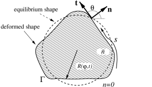
FIG. 1.: A charged incompressible liquid in a magnetic field. We assume a piecewise constant electron density ($n\!=\!\bar{n}$ inside, while $n\!=\!0$ outside the droplet). The parameterization $R(\varphi,t)$, the tangent ${\bf t}$ and normal ${\bf n}$ unit vectors to the boundary $\Gamma$ are indicated; $s$ is the arc-length and $\theta$ the tangent angle.

Let us now concentrate on the “internal” velocity given by the first term in Eq. (11). We should note that the neglected external velocity ${\bf v}_{\rm ext}$ derived from the confining field [Eq. (10)] is important for long term stability of the system, and will modify the propagation velocity. In general, it could also change the shape of the modes, yet one can devise situations in which this effect is not important, i.e. a linear confining potential in a rectilinear infinite edge, or a parabolic potential for a circular droplet.

For an incompressible 2DES with a piecewise constant density, the density can be taken outside the integral; then using Stokes’ theorem, the area integral can be transformed into a line integral over the boundary $\Gamma\!=\!\partial{\cal A}$ of the electron liquid:

$${\bf v({\bf r})}=\frac{\bar{n}e^{2}}{\epsilon m_{e}\omega_{c}}\oint_{\Gamma}ds^{\prime}\,\frac{{\bf t}(s^{\prime})}{|{\bf r}-{\bf r}(s^{\prime})|}\,.$$ (12)

Here ${\bf t}(s^{\prime})$ is the unit tangent vector at arc-length $s^{\prime}$:

$$\begin{array}[]{l}{\bf t}(s^{\prime})=\partial_{s^{\prime}}{\bf r}(s^{\prime})\equiv{\bf r}_{s^{\prime}}\,,\\ {\bf n}(s^{\prime})\equiv-{\bf e}_{z}\times{\bf t}(s^{\prime})\,,\end{array}$$ (13)

and we defined the unit normal vector ${\bf n}(s^{\prime})$ for later use. The short distance singularity in the integrand is cut off at a length scale $r_{0}$. Equation (12) forms the basis of our contour dynamics treatment—it expresses the velocity of the edge in terms of a nonlocal self-interaction of the edge.

We see that: (i) the dynamics is chiral, being determined by the tangent vector; (ii) the fluid contained within $\Gamma$ is incompressible, so that the area is conserved. It is interesting to note similar traits were found in the past for the dynamics of vortex patches;[9, 10, 11, 12] indeed, it is this analogy which inspired the present work. A detailed description of the vortex patch case, and stressing the similarities and differences with the shape deformations of the 2DES is presented for completeness in Appendix B.

IV Kinematics of uniformly propagating deformations

Having determined the velocity of the electron liquid, we now focus on the motion of the 2DES boundary $\Gamma$. The velocity of a point on the boundary can be written in terms of the normal and tangential components,

$${\bf v}=U(s)\,{\bf n}+W(s)\,{\bf t}.$$ (14)

The tangential velocity $W(s)$ is largely irrelevant, as it solely accounts for a reparametrization of the curve; the boundary motion is determined by the normal component of the velocity.

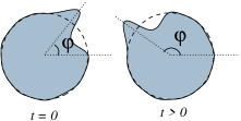
FIG. 2.: A uniformly propagating edge deformation. The boundary satisfies $R(\varphi,t)=R(\varphi-\Omega t)$.

We now ask whether there are modes which propagate along the boundary with no change in shape. Previous work [17] has focused on small perturbations of a straight, infinite edge. Here we consider deformations of a circular droplet of incompressible electrons (the non-linear deformation of a straight infinite edge is discussed in Appendix F). A uniformly propagating mode is, in this case, characterized by a boundary that moves like a rotating rigid body (see Fig. 2), namely, the radius of the boundary satisfies

$$R(\varphi,t)=R(\varphi-\Omega t)\,,$$ (15)

where $\varphi$ is the azimuthal angle, and $\Omega$ is the angular frequency of the boundary rotation. This translates into a condition for the normal velocity:

$$U\equiv\left.{\bf n}({\bf r})\cdot{\bf v}({\bf r})\right|_{{\bf r}\in\Gamma}=\Omega\;{\bf n}({\bf r})\cdot\left({\bf e}_{z}\times{\bf r}\right)\,.$$ (16)

We seek surface shapes $R(\varphi)$ (see Figs. 1 and 2) that rotate uniformly, satisfying Eq. (16). Consider the following parameterization of the surface:

$$R(\varphi)=R_{0}\left(1+\sum_{l=-\infty}^{\infty}b_{l}\;e^{il\varphi}\right).$$ (17)

In this parametrization, we can write the unit tangent vector explicitly as

$${\bf t}(\varphi)=\frac{\mbox{\boldmath${\tau}$}(\varphi)}{|\mbox{\boldmath${\tau}$}(\varphi)|}\,,$$ (18)

where

$$\mbox{\boldmath${\tau}$}(\varphi)\equiv\frac{\partial{\bf r}(\varphi)}{\partial\varphi}={\bf e}_{r}R^{\prime}(\varphi)+{\bf e_{\varphi}}R(\varphi)\,.$$ (19)

Likewise, the unit normal vector is given by

$${\bf n}(\varphi)=-{\bf e}_{z}\times\frac{\mbox{\boldmath${\tau}$}(\varphi)}{|\mbox{\boldmath${\tau}$}(\varphi)|}\,.$$ (20)

Given the identity ${\bf r}_{s}\,ds\!=\!{\bf r}_{\varphi}\,d\varphi$, the normal velocity of the boundary, derived from Eq. (12), can be written as

$$U(\varphi)=\frac{\bar{n}e^{2}}{\epsilon m_{e}\omega_{c}}\int_{0}^{2\pi}\!d\varphi^{\prime}\;\frac{{\bf n}(\varphi)\cdot\mbox{\boldmath$\tau$}(\varphi^{\prime})}{|{\bf R}(\varphi)-{\bf R}(\varphi^{\prime})|}\,,$$ (21)

while inserting Eqs. (19) and (20) into Eq. (16) yields

$$U(\varphi) = \Omega\;{\bf n}({\bf R})\cdot\left({\bf e}_{z}\times{\bf R}\right)$$ (22)

$$= -\frac{i\Omega}{|\mbox{\boldmath${\tau}$}(\varphi)|}\left[\sum_{l}l\,b_{l}\,e^{il\varphi}+\sum_{l}\sum_{p}\frac{l}{2}\,b_{l\!-\!p}b_{p}\,e^{il\varphi}\right].$$ (23)

We seek frequencies $\Omega$ and coefficients $b_{l}$ that satisfy Eqs. (21) and (22). The solutions to this non-linear eigenvalue problem represent edge modes that propagate without any dispersion.

V Solving the non-linear eigenvalue problem—perturbative approach

Unfortunately, it has not been possible to solve exactly the non-linear eigenvalue problem for $b_{l}$ and $\Omega$ as written in Eqs. (21) and (22). We therefore seek a perturbative solution by expanding the right-hand side of Eq. (21) in powers of $b_{l}$. This allows us to to go beyond the linear approximations used in the past, and we have succeeded in calculating shape deformations to ${\cal O}[b_{l}^{4}]$ and angular frequencies to ${\cal O}[b_{l}^{5}]$. Expanding the non-linear eigenvalue problem to fifth order, we find the condition

$$\tilde{\Omega}\left(b_{l}+\frac{1}{2}\sum_{p}b_{l-p}b_{p}\right) = Q_{l}\,b_{l}+\sum_{p}R_{l\!-\!p,p}\,b_{l-p}b_{p}+\!\sum_{p,q}S_{l\!-\!p,p\!-\!q,q}\,b_{l-p}b_{p-q}b_{q}$$ (25)

$$+\!\sum_{p,q,r}T_{l\!-\!p,p\!-\!q,q\!-\!r,r}\,b_{l-p}b_{p-q}b_{q-r}b_{r}+\!\!\!\sum_{p,q,r,s}U_{l\!-\!p,p\!-\!q,q\!-\!r,r\!-\!s,s}b_{l-p}b_{p-q}b_{q-r}b_{r-s}b_{s}+{\cal O}[b_{l}^{6}]\,,$$

where

$$\tilde{\Omega}=\frac{\epsilon m_{e}\omega_{c}R_{0}}{\bar{n}e^{2}}\,\Omega,$$ (26)

and the “matrix elements” $Q$, $R$, $S$, $T$ and $U$ are obtained from Eq. (21) in Appendix A.

Since the equation to be solved results from an expansion in powers of $b_{l}$, it is sufficient to solve Eq. (25) perturbatively, by expanding in powers of the largest coefficient $b_{L}$. Let us assume that

$${b_{l}}\,\left\{\begin{array}[]{ll}={\cal O}[\delta]\,,&\;\;{\rm for}\;\;l=\pm L\,,\\ ={\cal O}[\delta^{2}]\,,&\;\;{\rm for}\;\;l\neq\pm L\,.\end{array}\right.$$ (27)

We then consider an expansion of the coefficients $b_{l}$ and eigenvalue $\tilde{\Omega}$ in powers of $\delta$:

$${b_{l}}=\left\{\begin{array}[]{ll}b^{(1)}_{L}\,,&\;\;{\rm for}\;\;l=\pm L\,,\\ b^{(2)}_{l}+b^{(3)}_{l}+\cdots\,,&\;\;{\rm for}\;\;l\neq\pm L\,.\end{array}\right.$$ (30)

$$\tilde{\Omega}_{L}=\tilde{\Omega}_{L}^{(0)}+\tilde{\Omega}_{L}^{(1)}+\tilde{\Omega}_{L}^{(2)}+\cdots\,$$ (31)

where $b^{(k)}$ and $\tilde{\Omega}^{(k)}$ are of order ${\cal O}[\delta^{k}]$. By substituting expressions (30) and (31) into Eq. (25), and grouping terms order by order, we find that:

1. The first-order term yields the dispersion relation in the linear approximation:

   $$\tilde{\Omega}^{(0)}[L]=Q_{L}\,;$$ (32)

2. Second-order terms couple the fundamental and second harmonics of the deformation, with no correction to the eigenvalue:

   $$\tilde{\Omega}^{(1)}[L]=0\,,$$ (33)

   $$b^{(2)}_{\pm 2L}=\frac{1}{2}\,\frac{2R_{L,L}-Q_{L}}{Q_{L}-Q_{2L}}\,[b_{L}^{(1)}]^{2}\,,$$ (34)

   $$b^{(2)}_{l}=0\,,\;\;{\rm for}\;\;l\neq\pm 2L\,;$$ (35)

3. Third-order terms give the first correction to the frequency and couple the first and third harmonics:

   $$\tilde{\Omega}^{(2)}[L]=3S_{L,L,-L}[b_{L}^{(1)}]^{2}+(2R_{2L,-L}-Q_{L})b_{2L}^{(2)}\,,$$ (36)

   $$b^{(3)}_{\pm 3L}=\frac{(2R_{2L,L}-Q_{L})b_{2L}^{(2)}b_{L}^{(1)}+S_{L,L,L}[b_{L}^{(1)}]^{3}}{Q_{L}-Q_{3L}}\,,$$ (37)

   $$b^{(3)}_{l}=0\,,\;\;{\rm for}\;\;l\neq\pm 3L\;;$$ (38)

4. Fourth-order terms provide coupling to both second and fourth harmonics:

   $$\tilde{\Omega}^{(3)}[L]=0\,,$$ (39)

   $$b^{(4)}_{\pm 2L}=\frac{1}{Q_{L}-Q_{2L}}\left\{(2R_{3L,-L}-Q_{L})b^{(3)}_{3L}b_{L}^{(1)}-\tilde{\Omega}^{(2)}[L]\left(b^{(2)}_{2L}+\frac{[b_{L}^{(1)}]^{2}}{2}\right)+6S_{2L,L,-L}b^{(2)}_{2L}[b_{L}^{(1)}]^{2}+4T_{L,L,L,-L}[b_{L}^{(1)}]^{4}\right\}\!,$$ (40)

   $$b^{(4)}_{\pm 4L}=\frac{1}{Q_{L}-Q_{4L}}\left\{\frac{1}{2}(2R_{2L,2L}-Q_{L})[b^{(2)}_{2L}]^{2}+(2R_{3L,L}-Q_{L})b^{(3)}_{3L}b_{L}^{(1)}+3S_{2L,L,L}b^{(2)}_{2L}[b_{L}^{(1)}]^{2}+T_{L,L,L,L}[b_{L}^{(1)}]^{4}\right\}\!,\!\!\!$$ (41)

   $$b^{(4)}_{l}=0\,,\;\;{\rm for}\;\;l\neq\pm 4L\;;$$ (42)

5. The fifth-order term follows the same pattern. The couplings to higher harmonics is quite complex and we chose not to pursue it. We show only the correction to the eigenvalue:

   $$\tilde{\Omega}^{(4)}[L] = (2R_{2L,-L}-Q_{L})b^{(4)}_{2L}+(2R_{3L,-2L}-Q_{L})\frac{b^{(3)}_{3L}b^{(2)}_{2L}}{b^{(1)}_{L}}-\tilde{\Omega}^{(2)}[L]b^{(2)}_{2L}+3S_{3L,-L,-L}b^{(3)}_{3L}b^{(1)}_{L}$$ (44)

   $$+6S_{L,2L,-2L}[b^{(2)}_{2L}]^{2}+(12T_{2L,L,-L,-L}+4T_{-2L,L,L,L})b^{(2)}_{2L}[b_{L}^{(1)}]^{2}+10U_{L,L,L,-L,-L}[b_{L}^{(1)}]^{4}\,.$$

Note that the largest term in the perturbative expansion corresponds to the lowest harmonic and that higher order elements preserve the rotational symmetry $C_{L}$ (rotations by $2\pi/L$) of the initial term.

VI Solutions for the two-dimensional electron system

We now show some invariant shapes for the 2DES (see Secs. III and IV). Coefficients $b_{l}$ and frequencies $\tilde{\Omega}$ are obtained using the formulæ of Sec. V and matrix elements $Q$, $R$, $S$, $T$ and $U$ calculated in Appendix A.

Table I summarizes these results for states of rotational symmetry $C_{L}$, with $L$ = 2, 3, 4 and 5. Some particular shapes obtained from these coefficients and Eq. (17) are shown in Fig. 6 [for a comparison with similar states for vortex patches see Figs. 8 and 9].

For large deformations, the appearance of oscillations indicate that higher order terms are needed, since the perturbative method corresponds to a truncation of the Fourier decomposition [Eq. (17)]. An alternative approach, based on a local induction approximation, provides a better description in those cases. This alternative formulation is presented in Sec. VII.

It is interesting to note that the linear result for the frequency is [see Eqs. (32) and (A5)]

$$\tilde{\Omega}^{(0)}[l]=Q_{l}=4\sum_{k=2}^{|l|}\frac{1}{2k-1}\,,$$ (45)

where the last sum can be related to the digamma function [22] $\psi(|l|\!+\!{1/2})$. This linear result has been previously derived by several authors;[18] corrections are ${\cal O}[b_{l}^{2}]$. For a direct comparison with Eq. (8), which corresponds to the large-$l$ limit, we substitute the asymptotic expansion for the sum in Eq. (45); multiplication by $R_{0}$ yields the propagation velocity:

$$v_{g}=-2\ln\left(\frac{e^{-\gamma}}{4\,e^{2}|l|}\right)\frac{\bar{n}e^{2}}{\epsilon m_{e}\omega_{c}}\,,$$ (46)

which closely corresponds to the group velocity $v_{g}\!\equiv\!\partial\omega_{0}(k)/\partial k$ obtained from Eq. (8) after the substitution $l\!\sim\!ka$. The dispersion for these linear edge excitations has been confirmed experimentally in both the frequency [23] and time [21, 24, 25] domains.

TABLE I.: Stationary deformations of a two-dimensional electron system. Angular frequencies and lowest harmonics of the deformation for $L\!=\!2,3,4,5$.

$\;\;l\;\;$	${\tilde{\Omega}=({\epsilon m_{e}\omega_{c}R_{0}}/{\bar{n}e^{2}})\,\Omega}$	$b_{2l}$	$b_{3l}$	$b_{4l}$
2	$\frac{4}{3}-5.09048\,b_{2}^{2}-16.1333\,b_{2}^{4}$	$\frac{29}{24}\,b_{2}^{2}+1.86911\,b_{2}^{4}$	$0.911769\,b_{2}^{3}$	$-0.345388\,b_{2}^{4}$
3	$\frac{32}{5}-16.8464\,b_{3}^{2}+39.6332\,b_{3}^{4}$	$1.63473\,b_{3}^{2}+8.36452\,b_{3}^{4}$	$1.97442\,b_{3}^{3}$	$-0.540557\,b_{3}^{4}$
4	$\frac{284}{105}-30.0989\,b_{4}^{2}-154.821\,b_{4}^{4}$	$1.94074\,b_{4}^{2}+24.3045\,b_{4}^{4}$	$2.56102\,b_{4}^{3}$	$-3.45272\,b_{4}^{4}$
5	$\;\frac{992}{315}-45.5507\,b_{5}^{2}-418.524\,b_{5}^{4}\;$	$\;2.17945\,b_{5}^{2}+50.1748\,b_{5}^{4}\;$	$\;2.74603\,b_{5}^{3}$	$-9.80691\,b_{5}^{4}\;$

VII Local induction approximation

As we have seen, the motion of the edge is determined by the velocity of the fluid at the surface. The nonlocal equation for the velocity of the boundary, Eq. (12), can be turned into a differential equation for the curvature of the boundary if we concentrate on the local contributions. This local induction approximation (LIA) [26] was explored by Goldstein and Petrich in a series of papers dealing with the evolution of vortex patches.[12, 16] The situation is considerably more favorable in this problem, due to the more rapid decay of the interaction [$1/r$ for charges vs. $\ln(r)$ for vortices, see Eqs. (12) and (B3)]. Figure 1 defines most terms used in this section.

The LIA corresponds to the introduction of a large distance cut-off $\Lambda$ in the expression for the velocity of the boundary ${\bf v}[{\bf r}(s)]$ [Eq. (12)]:

$$\oint_{\Gamma}\{\cdots\}\,ds^{\prime}\;\mbox{\boldmath${\longrightarrow}$}\;\int_{s-\Lambda/2}^{s+\Lambda/2}\!\!\!\!\{\cdots\}\,ds^{\prime}\,.$$ (47)

The line integral in Eq. (12) is then calculated by expanding the integrand in powers of $\Delta\!\equiv\!(s^{\prime}\!-\!s)$. By using the Frenet-Serret relations

$$\begin{array}[]{l}{\bf r}_{s}={\bf t}\,,\\ {\bf t}_{s}=-\kappa\,{\bf n}\,,\\ {\bf n}_{s}=\kappa\,{\bf t}\,,\end{array}$$ (48)

where $\kappa\!=\!\theta_{s}$ is the local curvature of the boundary, we obtain

$${\bf t}(s^{\prime}) \simeq {\bf t}(s)\left[1-\frac{\Delta^{2}}{2}\kappa^{2}-\frac{\Delta^{3}}{2}\kappa\kappa_{s}+...\right]$$ (50)

$$+{\bf n}(s)\left[-\Delta\,\kappa-\frac{\Delta^{2}}{2}\kappa_{s}+\frac{\Delta^{3}}{6}(\kappa^{3}-\kappa_{ss})+...\right]\,,$$

$${\bf r}(s^{\prime}) - {\bf r}(s)\simeq{\bf t}(s)\left[\Delta-\frac{\Delta^{3}}{6}\kappa^{2}-\frac{\Delta^{4}}{8}\kappa\kappa_{s}+...\right]$$ (52)

$$+{\bf n}(s)\left[-\frac{\Delta^{2}}{2}\kappa-\frac{\Delta^{3}}{6}\kappa_{s}+\frac{\Delta^{4}}{24}(\kappa^{3}-\kappa_{ss})+...\right]\,.$$

To lowest order the normal and tangential velocities then are given by:

$$U_{\rm LIA}=-\left[\frac{\bar{n}e^{2}}{\epsilon m_{e}\omega_{c}}\right]\frac{\Lambda^{2}}{8}\,\kappa_{s}\,,$$ (53)

$$W_{\rm LIA}=\left[\frac{\bar{n}e^{2}}{\epsilon m_{e}\omega_{c}}\right]\left(\ln\frac{\Lambda^{2}}{2r_{0}}-\frac{11\Lambda^{2}}{96}\,\kappa^{2}\right).$$ (54)

It is worth noting that since the rate of change of the area ${\cal A}$ of the droplet is ${\cal A}_{t}\!=\!\oint ds\,U(s)$ [see Eq. (D8)], the LIA with $U_{\rm LIA}\!\propto\!\kappa_{s}$ (or any exact differential) automatically conserves area. This is not surprising since we started with an incompressible system, but shows that the local approximation used has not introduced an obvious error. It is also interesting to realize that the perimeter ${\cal L}$ of the curve derived from these velocities is conserved as well: ${\cal L}_{t}\!=\!\oint ds\,(\kappa U+W_{s})=0$ [see Eq. (D7)].

The time evolution of a curve in two dimensions is given quite generally by the integro-differential equation [16, 27] (see Appendix D)

$$\kappa_{t}=-[\kappa^{2}+\partial_{ss}]U+\kappa_{s}W-\kappa_{s}\int_{0}^{s}[\kappa U+W_{s^{\prime}}]ds^{\prime}\,.$$ (55)

We now introduce the results from Eq. (53). A “gauge” change, realized by modifying $W$ so that the integrand of Eq. (55) vanishes, eliminates the remaining non-local dependences and yields

$$\kappa_{t}=\left[\frac{\bar{n}e^{2}}{\epsilon m_{e}\omega_{c}}\right]\frac{\Lambda^{2}}{8}\left(\frac{3}{2}\kappa^{2}\kappa_{s}+\kappa_{sss}\right).$$ (56)

After a simple time rescaling, the curvature satisfies the mKdV equation:[15]

$$\kappa_{t}=\frac{3}{2}\kappa^{2}\kappa_{s}+\kappa_{sss}\,.$$ (57)

The mKdV dynamics are integrable, with an infinite number of globally conserved geometric quantities,[12] the most important of which are the center of mass, area, and angular momentum of the droplet.

The mKdV equation possesses a variety of soliton solutions, including traveling wave solutions and propagating “breather” solitons (see Appendix F). Here we will focus on the traveling wave solutions of Eq. (57) of the form

$$\kappa(s,t)=\kappa(z)\,,\;\;\;\;{\rm with}\;\;z\equiv s-c\,t\,,$$ (58)

which represents uniformly rotating deformed droplets (see Fig. 3). The ordinary differential equation for $\kappa(z)$ can be integrated twice with the result

$$\frac{1}{2}(\kappa^{\prime})^{2}=-\frac{1}{8}\kappa^{4}+\frac{1}{2}c\kappa^{2}+a\kappa-2b\,,$$ (59)

where $a$ and $b$ are constants of integration ($a\!=\!b\!=\!0$ for infinite systems, see Appendix F). This ordinary differential equation can be easily integrated:

$$z-z_{0}=\pm\int_{\kappa_{0}}^{\kappa}\frac{d\kappa^{\prime}}{\sqrt{-V(\kappa^{\prime})}}\,,$$ (60)

$$V(\kappa)=\frac{\kappa^{4}}{4}-c\,\kappa^{2}-2a\,\kappa+4b\,.$$ (61)

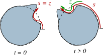
FIG. 3.: A uniformly propagating edge deformation. The curvature satisfies $\kappa(s,t)=\kappa(z)$, with $z=s-c\,t$.

This problem is thus analogous to a particle moving in a quartic potential (Fig. 4). The integrals involved can be expressed in terms of elliptic integrals [22] and depend crucially on the nature and location of the zeros of $V(\kappa)$. For curves with finite perimeter and no self-crossings we find that it is necessary to have two real and two complex zeros: $\kappa_{\rm max}$, $\kappa_{\rm min}$, and $-(\kappa_{\rm max}\!+\!\kappa_{\rm min})/2\!\pm\!i\xi$ (see Appendix E). Note that $\kappa_{\rm max}$ and $\kappa_{\rm min}$ correspond to the maximum and minimum curvatures of the boundary.

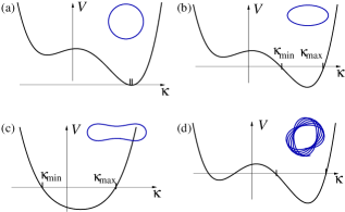
FIG. 4.: Some possible potentials $V(\kappa)$ and corresponding schematic solutions for the shape of the boundary. Potentials with two real zeros may have physical solutions: (a) Curvature is fixed, the solution is a circle; (b) Curvature is positive definite, the boundary is convex; (c) Positive and negative curvatures. (c) Potentials with four zeros have solutions with unphysical self-intersections.

The periodic solutions of Eq. (60), expressed in terms of Jacobi elliptic functions,[22] are given by (Appendix E):

$$\kappa(z)=\frac{(q\kappa_{\rm max}\!+\!p\kappa_{\rm min})+(p\kappa_{\rm min}\!-\!q\kappa_{\rm max})\,{\rm cn}\!\left(\!\sqrt{pq}\frac{\displaystyle z}{2}\,|\,\lambda\right)}{(p+q)+(p-q)\,{\rm cn}\!\left(\!\sqrt{pq}\frac{\displaystyle z}{2}\,|\,\lambda\right)},$$ (62)

where

$$p = \sqrt{(3\kappa_{\rm max}+\kappa_{\rm min})^{2}+\xi^{2}}\,,$$ (63)

$$q = \sqrt{(\kappa_{\rm max}+3\kappa_{\rm min})^{2}+\xi^{2}}\,,$$ (64)

$$\lambda = \sqrt{\left[(\kappa_{\rm max}-\kappa_{\rm min})^{2}-(p-q)^{2}\right]/4pq}\,.$$ (65)

The free parameter $\xi$ is actually determined by the boundary conditions. The period of $\kappa$ is given by the elliptic integral

$$L_{\kappa}=\frac{8}{\sqrt{pq}}\,K(\lambda)\,.$$ (66)

We now require that the tangent angle increases by a factor of $2\pi$ after an integer multiple $l$ curvature periods, so that the curve is closed and with no self crossings (see Fig. 5):

$$\theta(l\,\!L_{\kappa})=\int_{0}^{l\,\!L_{\kappa}}\!\!\!\kappa(s)\,ds=2\pi\,.$$ (67)

It is evident that the resulting curves are invariant under rotations by $2\pi/l$, that is the curves have $C_{l}$ symmetry. The curves thus generated can be characterized by $(l,\kappa_{\rm max},\kappa_{\rm min})$ or more conveniently, although indirectly, by the symmetry, the area and the perimeter of the curve.

FIG. 5.: Illustration of the boundary conditions implied by Eq. (67). Top: after $l$ periods $L_{\kappa}$ of the curvature $\kappa(s)$, the tangent angle $\theta$ increases by precisely $2\pi$. Bottom: the resulting deformed boundary.

The contour shape can be easily determined once the tangent angle $\theta(s)$ is known as a function of arc-length. Since $dz\equiv dx+i\,dy=\exp[{i\,\theta(s)}]\,ds$, we have

$$z(s)\equiv x(s)+i\,y(s)=\int_{0}^{s}e^{i\,\theta(s^{\prime})}\,ds^{\prime}\,.$$ (68)

The full lines in Fig. 6 show some uniformly rotating soliton shapes, calculated from Eqs. (62) and (68). These are essentially identical with Goldstein and Petrich’s [16] soliton solutions for the vortex patch problem, but the more local nature of the interaction in the 2DES case should guarantee a better correspondence with the exact solutions including non-local terms. Indeed, the curves resulting from the perturbative method and the LIA are quite close, even for considerable deformations of the boundary. For larger deformations the perturbative results show artifacts due to the limited number of Fourier components. The advantage of the LIA becomes evident in this case, since it is an expansion in powers of the curvature and not the deformation, and thus allows for relatively large long-wavelength deformations. More significantly, the LIA and the resulting integrable dynamics allow one to uncover geometrical conservation laws which would be hidden in a perturbative calculation.[28] This advantage comes at a price: the detailed information on frequencies is obscured by the introduction of the long distance cut-off $\Lambda$ and by the gauge transformation of the tangential velocity $W$, while the frequency is easily obtained in the perturbative calculation.

FIG. 6.: Uniformly rotating shapes of a 2DES. Solid lines: solutions of the mKdV equation obtained from the local induction approximation. Dotted lines: solutions obtained using the perturbative expansion. The values of the coefficient $b_{l}$, and the ratio of curvatures $\sigma\!\equiv\!\kappa_{\rm min}/\kappa_{\rm max}$ are: (a) $b_{2}\!=\!0.073,\,\sigma\!=\!0.4$; (b) $b_{2}\!=\!0.19,\,\sigma\!=\!0$; (c) $b_{2}\!=\!0.36,\,\sigma\!=\!-\!0.2$; (d) $b_{3}\!=\!0.027,\,\sigma\!=\!0.4$; (e) $b_{3}\!=\!0.10,\,\sigma\!=\!-\!0.2$; (f) $b_{3}\!=\!0.29,\,\sigma\!=\!-\!0.45$; (g) $b_{4}\!=\!0.014,\,\sigma\!=\!0.4$; (h) $b_{4}\!=\!0.089,\,\sigma\!=\!-\!0.4$; (i) $b_{4}\!=\!0.24,\,\sigma\!=\!-\!0.56$.

VIII Conclusions

A contour dynamics formulation of the excitations on the edge of a two-dimensional electron system in a magnetic field has allowed us to demonstrate the existence, beyond the usual linear regime, of shape deformations that propagate uniformly. A local approximation to the nonlocal dynamics shows that the curvature of the edge of the droplet obeys the modified Korteweg-de Vries equation, which has integrable dynamics and soliton solutions. Earlier studies [29] of edge channels in QH samples have shown the presence of nonlinear waves, but in Ref. [29] the nonlinearity originates in the variations of the strength of the confining field (the ${\bf E}_{\rm ext}$ of Sec. II), whereas here we concentrate on nonlinear effects originating in geometrical effects.

Since these solutions are dispersionless, it may be possible to distinguish them from linear edge waves in time-of-flight measurements of the type depicted in Fig. 7. In a circular QH system[24] a voltage pulse applied to a gate produces an edge deformation. The deformation propagates along the edge of the system in one direction and is detected, i.e. by means of a capacitive probe. For this geometry, the pulse comes back repeatedly and it is possible to observe it after numerous passes. While a gradual decrease of the amplitude is always expected due to residual dissipation, dispersive and non-dispersive modes may be distinguished by the preservation of the general shape and width of the non-dispersive modes.

On the theoretical side, it would be interesting to connect our hydrodynamic treatment of these edge solitons with field-theoretical treatments of edge excitations.[18, 19]

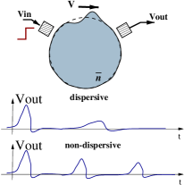
FIG. 7.: Soliton excitations travel without shape changes. In a circular QH system[24] with non-contact probes it is possible to observe repeated signals. While a gradual decrease of the amplitude is always expected due to residual dissipation, dispersive and non-dispersive modes may be distinguished by the preservation of the general shape and width of the non-dispersive modes.

 

A Matrix elements for the non-linear eigenvalue problem

In order to determine the matrix elements $Q$, $R$, $S$, $T$ and $U$ for the non-linear eigenvalue problem [Eq. (25)], we need to expand Eq. (21) in powers of the coefficients $b_{l}$ of the parametrization [Eq. (17)]. We initially realize that

$${\bf n}(\varphi){\bf\cdot}\mbox{\boldmath${\tau}$}(\varphi+\omega) = \frac{1}{|\mbox{\boldmath${\tau}$}(\varphi)|}\Biggl{\{}-\sin\omega-2\sum_{l}b_{l}\,e^{il\varphi}\left[\cos\frac{l\omega}{2}\,\sin\omega+l\cos\omega\,\sin\frac{l\omega}{2}\right]+$$ (A2)

$$+\sum_{l,p}b_{l\!-\!p}b_{p}\,e^{il\varphi}\left[(lp\!-\!p^{2}\!-\!1)\,\cos\frac{(l\!-\!2p)\omega}{2}\,\sin\omega\!-\!(l\!-\!2p)\,\cos\omega\,\sin\frac{(l\!-\!2p)\omega}{2}\right]\Biggr{\}},$$

$$|{\bf R}(\varphi+\omega)-{\bf R}(\varphi)|^{2} =$$ (A4)

$$4\sin^{2}\frac{\omega}{2}\left[1+2\sum_{l}b_{l}\,e^{il\omega/2}\,\cos\frac{\omega}{2}-\sum_{l,p}b_{l\!-\!p}b_{p}\,e^{il\omega/2}\,\frac{\sin\frac{(l-p+1)\omega}{2}\,\sin\frac{(p-1)\omega}{2}+\sin\frac{(l-p-1)\omega}{2}\,\sin\frac{(p+1)\omega}{2}}{2\sin^{2}\frac{\omega}{2}}\right].$$

By expanding ${\bf n}(\varphi){\bf\cdot}\mbox{\boldmath${\tau}$}(\varphi+\omega)/|{\bf R}(\varphi+\omega)-{\bf R}(\varphi)|$ in powers of $b_{l}$, and integrating over $\omega$ [see Eq. (21)], one obtains the relevant matrix elements $Q$, $R$, $S$, $T$ and $U$. All integrals converge without the need for short distance cut-offs. The three lowest order terms can be written as follows:

$$Q_{l} = 4\sum_{k=2}^{|l|}\frac{1}{2k-1}\,,$$ (A5)

$$R_{l-p,p} = \sum_{k=1}^{|l|}\frac{1}{2k-1}-\sum_{k=1}^{|l-p|}\frac{1}{2k-1}-\sum_{k=1}^{|p|}\frac{1}{2k-1}\,,$$ (A6)

$$S_{l\!-\!p,p\!-\!q,q} = -\frac{5}{l}\left[{\frac{l}{1-4{l^{2}}}}+{\frac{p}{1-4{p^{2}}}}+{\frac{q}{1-4{q^{2}}}}+{\frac{l-p}{1-4{{(l-p)}^{2}}}}+{\frac{l-q}{1-4{{(l-q)}^{2}}}}+{\frac{p-q}{1-4{{(p-q)}^{2}}}}+{\frac{l-p+q}{1-4{{(l-p+q)}^{2}}}}\right]$$ (A9)

$$+\frac{1}{12}\left[-(3+4l^{2})\sum_{k=1}^{|l|}\frac{1}{2k-1}-(1+4p^{2})\sum_{k=1}^{|p|}\frac{1}{2k-1}+(5+4q^{2})\sum_{k=1}^{|q|}\frac{1}{2k-1}+[5+4(l-p)^{2}]\sum_{k=1}^{|l-p|}\frac{1}{2k-1}\right.$$

$$\left.-[1+4(l-q)^{2}]\sum_{k=1}^{|l-q|}\frac{1}{2k-1}+[5+4(p-q)^{2}]\sum_{k=1}^{|p-q|}\frac{1}{2k-1}-[1+4(l-p+q)^{2}]\sum_{k=1}^{|l-p+q|}\frac{1}{2k-1}\right]\,.$$

Higher order terms are long and uninspiring.

B Comparison with the vortex patch case

For the sake of comparison, we draw analogy to the case of a vortex patch, a two-dimensional, bounded region of constant vorticity $\omega_{p}$ surrounded by an irrotational fluid.[9] The vorticity can either be distributed, as in a regular fluid, or concentrated in individual vortices, in the case of a superfluid (in this case it is clear that the hydrodynamic treatment will be valid only for length-scales larger than the inter-vortex spacing). The important thing is that in ideal fluids the area of the vortex patch is conserved due to Kelvin’s circulation theorem,[26] and therefore the vortex patch is essentially incompressible. Figure 1 can be used to describe this case by replacing the electron density $n$ by the vorticity $\omega_{p}$.

The steady state solution in this case is clearly a circle, and small deformations of the boundary travel along the boundary itself, as has been known for a long time.[9] One can also ask what happens when the deformations are large: are there modes that do not change shape, i.e., solitons? One such solution has been known since Kirchhoff’s time: an ellipse with constant vorticity will rotate uniformly in an ideal fluid. Numerical calculations by Deem and Zabusky [12, 11] in the 70’s obtained additional invariant shapes.

For inviscid incompressible fluids, the equations of motion for the fluid are simply given by:

$$\mbox{\boldmath${\nabla}$}\cdot{\bf v}=0\,,$$ (B1)

$$\mbox{\boldmath${\nabla}$}\times{\bf v}=\omega\,,$$ (B2)

where $\omega$ is the vorticity. Assuming that the velocity far from the patch vanishes, the velocity of the fluid in presence of a region of finite vorticity $\omega_{p}$ can be expressed as

$${\bf v_{v}}({\bf r})=-\frac{\omega_{p}}{2\pi}\oint_{\Gamma}ds^{\prime}\,{\bf t}(s^{\prime})\,\ln\left[{|{\bf r}-{\bf r}(s^{\prime})|\over r_{0}}\right].$$ (B3)

The arguments presented in Secs. III and IV are now applied mutatis mutandis to this case. The only difference with the 2DES comes from the fact that the kernel in the interaction is now logarithmic, and Eq. (12) is then replaced by Eq. (B3). We see that, as in the 2DES case (Secs. III and IV), the dynamics is chiral, being determined by the tangent vector; and since the fluid contained within $\Gamma$ is incompressible the area is conserved. The normal velocity of the contour is then given by

$$U_{\rm v}(\varphi)=-\frac{\omega_{p}}{2\pi}\int_{0}^{2\pi}\!\!d\varphi^{\prime}\,{\bf n}(\varphi)\cdot\mbox{\boldmath${\tau}$}(\varphi^{\prime})\ln\left[\frac{|{\bf R}(\varphi)-{\bf R}(\varphi^{\prime})|}{r_{0}}\right]\!.$$ (B4)

As before, we seek solutions that satisfy Eqs. (16) [or (22)] and (B4). First, we follow the procedure of Appendix A to determine the matrix elements $Q$, $R$, $S$, $T$ and $U$. The first few of these are given by

$$Q^{V}_{l} = \frac{1}{2}-\frac{1}{2|l|}\,,$$ (B5)

$$R^{V}_{l,p} = -\frac{1}{4|l|}\,.$$ (B6)

$$S^{V}_{l\!-\!p,p\!-\!q,q} = \frac{1}{12}\Bigl{[}1-|l|-|l-p|+|2l-p|+|l-q|$$ (B9)

$$-|2l-q|-|p-q|+|l+p-q|$$

$$+\delta(2l-p)+\delta(l-q)+\delta(l+p-q)\Bigr{]}\,.$$

We then apply the results of Sec. V, to determine the amplitude of the lowest harmonics for the vortex-patch case, using the appropriate matrix elements [Eqs. (B5)–(B9)]. These results are summarized in Table II, and some of the resulting invariant shapes are shown in Figs. 8 and 9.

It has long been known [9] that an elliptical region of vorticity in an otherwise irrotational fluid, namely the Kirchhoff ellipse, rotates uniformly with angular frequency $\Omega\!=\!(\omega_{p}/4)(1\!-\!b^{2}/a^{2})$, where $(a\!+\!b)$ and $(a\!-\!b)$ represent the maximum and minimum radii respectively (see Appendix C). A simple analysis shows that both frequency and angular components $b_{l}$ shown in Table II exactly match a series expansion of the ellipse. Figure 8 compares the perturbative results with the exact solution. Even for relatively high deformations both results are in reasonable agreement.

FIG. 8.: The $l\!=\!2$ stationary deformations of a vortex patch. Dotted line: the Kirchoff ellipse. Full line: perturbative solution. (a) $b_{2}\!=\!0.2$, (b) $b_{2}\!=\!0.3$.

In the case of deformations with higher angular dependences there are no analytic solutions beyond the linear approximation. In this case, the angular frequencies are given[9] to zeroth-order in the deformation by $\Omega\!=\!(m\!-\!1)/2m$, which coincides with the values for $Q^{V}_{l}$ [see Eqs. 32 and B5]. Numerical solutions by Deem and Zabusky [11] for $l\!=\!3,4$ also compare favorably with the perturbative results, as can be seen in Fig. 9. In fact, the angular velocities determined from Table II coincide with those shown in Ref. [11] to all significant figures of that paper.

TABLE II.: Stationary deformations of a vortex patch. Angular frequencies and lowest harmonics of the deformation for $L\!=\!2,3,4,5$ [the equivalent results for the 2DES are summarized in Table I].

$\;\;l\;\;$	${\tilde{\Omega}=\Omega/\omega_{p}}$	$b_{2l}$	$b_{3l}$	$b_{4l}$
2	$\frac{1}{4}-b_{2}^{2}+b_{2}^{4}$	$\frac{3}{2}b_{2}^{2}-\frac{1}{2}b_{2}^{4}$	$\frac{5}{2}b_{2}^{3}$	$\frac{35}{8}b_{2}^{4}$
3	$\frac{1}{3}-2b_{3}^{2}-20b_{3}^{4}$	$\frac{5}{2}b_{3}^{2}+16b_{3}^{4}$	$8b_{3}^{3}$	$\frac{231}{8}b_{3}^{4}$
4	$\frac{3}{8}-3b_{4}^{2}-57b_{4}^{4}$	$\frac{7}{2}b_{4}^{2}+\frac{135}{2}b_{4}^{4}$	$\frac{33}{2}b_{4}^{3}$	$\frac{715}{2}b_{4}^{4}$
5	$\;\frac{2}{5}-4b_{5}^{2}-152b_{5}^{4}\;$	$\;\frac{9}{5}b_{5}^{2}+172b_{5}^{4}\;$	$\;28b_{5}^{3}$	$\frac{1615}{8}b_{5}^{4}\;$

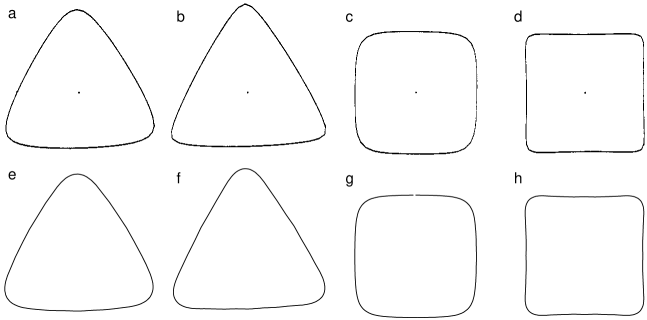
FIG. 9.: Vortex-patch “eigenstates” with $L\!=\!3$ and $L\!=\!4$. (a)-(d) Obtained numerically by Deem and Zabusky [figures are scanned from Ref. [11]]; (e)-(h) Determined perturbatively. The lowest harmonic $b_{L}$ is taken in each case from Table I of Ref. [11]: $b_{3}=0.096$, $b_{3}=0.11$, $b_{4}=0.048$ and $b_{4}=0.070$ respectively. The solutions are essentially identical and are too close to compare effectively in the same picture.

C The Kirchhoff ellipse as a solution of a contour dynamics problem

It is illustrative to show, starting from the contour dynamics, that an ellipse is indeed an invariant deformation for a vortex patch. Additionally it can be shown that this is an inherent property of the logarithmic kernel [Eq. B3] and that an ellipse it is not a solution for the 2DES.

Consider the following parametrization of an ellipse:

$$\begin{array}[]{l}x=(a+b)\cos\eta\,,\\ y=(a-b)\sin\eta\,.\end{array}$$ (C1)

It is evident that the radius is given by

$$r(\eta)=\sqrt{a^{2}+2ab\cos 2\eta+b^{2}}\,,$$ (C2)

and that tangential and normal vectors are given by

$${\tau} \equiv \frac{\partial{\bf r}}{\partial\eta}=-(a+b)\sin\eta\,{\bf e}_{x}+(a-b)\cos\eta\,{\bf e}_{y}\,,$$ (C3)

$${\bf n} = -\frac{{\bf e}_{z}\times\mbox{\boldmath${\tau}$}}{|\mbox{\boldmath${\tau}$}|}=\frac{(a-b)\cos\eta\,{\bf e}_{x}+(a+b)\sin\eta\,{\bf e}_{y}}{|\mbox{\boldmath${\tau}$}|}\,,$$ (C4)

where $|\mbox{\boldmath${\tau}$}|\!=\!\sqrt{a^{2}-2ab\cos 2\eta+b^{2}}\,$. The “rigid-body rotation” condition [Eq. (16)] can then be written as

$$U=\frac{\Omega}{|\mbox{\boldmath${\tau}$}(\eta)|}\,2ab\,\sin 2\eta\,.$$ (C5)

In addition the distance between two points on the ellipse takes the simple form

$$R^{2} \equiv |{\bf r}(\eta)-{\bf r}(\eta^{\prime})|^{2}$$ (C6)

$$= 4(a^{2}+b^{2})\sin^{2}\left(\frac{\eta-\eta^{\prime}}{2}\right)\left[1-\frac{2ab}{a^{2}+b^{2}}\cos(\eta+\eta^{\prime})\right]\!,$$ (C7)

and the dot product involved in Eqs. (21) and (B4) is given by

$${\bf n}(\eta)\cdot\mbox{\boldmath${\tau}$}(\eta^{\prime})=\frac{1}{|\mbox{\boldmath${\tau}$}(\eta)|}(a^{2}-b^{2})\sin(\eta-\eta^{\prime})\,.$$ (C8)

1 Vortex patches—exact solution

It is now simple to show that an ellipse is, indeed, a uniformly rotating shape for the vortex patch [Eqs. (16) and (B4)], since the normal velocity is given by

$$U_{\rm v} = -\frac{\omega_{p}}{4\pi|\mbox{\boldmath${\tau}$}(\eta)|}\,\int_{0}^{2\pi}\!\!\!d\eta^{\prime}\,\ln\left\{\left[4(a^{2}+b^{2})\sin^{2}(\frac{\eta-\eta^{\prime}}{2})\right]\times\left[1-\frac{2ab}{a^{2}+b^{2}}\cos(\eta+\eta^{\prime})\right]\right\}\sin(\eta-\eta^{\prime})$$ (C9)

$$= -\frac{\omega_{p}}{4\pi|\mbox{\boldmath${\tau}$}(\eta)|}\,\int_{0}^{2\pi}\!\!\!dx\,\ln\left[1-\frac{2ab}{a^{2}+b^{2}}\cos x\right]\times\left(\sin 2\eta\,\cos x-\cos 2\eta\,\sin x\right)\,,$$ (C10)

where in going from Eq. (C9) to (C10) we eliminated the term inside the first braces in the logarithm due to symmetry and changed variables to $x\!=\!\eta\!+\!\eta^{\prime}$. Finally, the term proportional to $\cos 2\eta$ vanishes upon integration and we are left with a simple integral, proportional to $\sin 2\eta$. As long as $a\!>\!b$ (for $a\!=\!b$ the ellipse has collapsed into a line), the integral exists in closed form:

$$U_{\rm v}={\omega_{p}}\,\frac{(a^{2}-b^{2})b}{2a|\mbox{\boldmath${\tau}$}(\eta)|}\,\sin 2\eta\,,$$ (C11)

which, by direct comparison with Eq. (C5), yields the angular velocity

$$\Omega_{\rm v}=\frac{\omega_{p}}{4}\left(1-\frac{b^{2}}{a^{2}}\right)\,.$$ (C12)

Consider now the parametrization given by Eq. (17) with $b_{l}$ given by the first row in Table II. The maximum and minimum radii correspond to $R(\varphi)$ for $\varphi$ equal to 0 and $\pi/2$ respectively (for $b_{2}>0$). It is easy to see that $a\!\sim\!1\!+\!3b_{2}^{2}\!-\!b_{2}^{4}$ and $b\!\sim\!2b_{2}\!+\!5b_{2}^{3}$, thus $\Omega/\omega_{p}\!\simeq\!1/2\!-\!b_{2}^{2}\!+\!b_{2}^{4}$, as shown in Table II. A simple Fourier analysis of Eq. (C2) also results in coefficients $b_{l}$ which agree with the perturbative solution.

2 Two dimensional electron systems—no exact solution

It is also simple to see why an ellipse is not a stationary solution of the two-dimensional electron system. Instead of the logarithm, one has to deal with $1/\sqrt{R^{2}}$, and the elimination of the first term inside the braces is not possible. The resulting integrands depend on $\eta$ in a non-trivial way, and the normal velocity is not proportional to $|{\mbox{\boldmath${\tau}$}}(\eta)|^{-1}\,\sin 2\eta$.

D Geometry of planar curve motion

For completeness, it is worth considering some general features of the planar curve motion.[27] Consider a curve described by some parametrization ${\bf r}(\alpha)$, where $\alpha$ is a parameter defined on a fixed interval (see Fig. 10). It is then possible to consider tangent and normal unit vectors defined by

$$\begin{array}[]{l}\displaystyle{\bf t}\equiv\frac{\mbox{\boldmath${\tau}$}(\alpha)}{|\mbox{\boldmath${\tau}$}(\alpha)|}\,,\;\;\;\;{\rm where}\;\;\mbox{\boldmath${\tau}$}(\alpha)={\bf r}_{\alpha}=\frac{\partial{\bf r}(\alpha)}{\partial\alpha}\,,\\ \displaystyle{\bf n}\equiv-{\bf e}_{z}\times{\mbox{\boldmath${t}$}}\,.\end{array}$$ (D1)

The arc-length $s(\alpha)$ corresponds to the length of the curve from some arbitrary point to ${\bf r}(\alpha)$ and is defined by $ds=\sqrt{dx^{2}+dy^{2}}=\sqrt{g}\,d\alpha$, where the metric $g$ is defined by $g\equiv\mbox{\boldmath${\tau\cdot\tau}$}$. We then have the Frenet-Serret relations

$$\begin{array}[]{l}{\bf r}_{s}={\bf t}\,,\\ {\bf t}_{s}=-\kappa\,{\bf n}\,,\\ {\bf n}_{s}=\kappa\,{\bf t}\,,\end{array}$$ (D2)

which define the curvature $\kappa$. It is also possible to define the curve in terms of its tangent angle $\theta(s)$, where $\theta_{s}=\kappa$.

FIG. 10.: Parametrization of a closed curve by a parameter $\alpha$ defined on a fixed interval. The illustration shows the arc-length $s$, the normal and tangential unit vectors ${\bf n}$ and ${\bf t}$ and the tangent angle $\theta$.

The kinematics of the curve can be determined if the velocity of the curve ${\bf r}_{t}$ is determined. It is convenient to decompose this velocity into its normal and tangential velocities (at fixed $\alpha$):

$${\bf r}_{t}=U\,{\bf n}+W\,{\bf t}\,.$$ (D3)

In general, $U$ and $W$ may be arbitrary functionals of ${\bf r}(s)$ and its derivatives. It is easy to show that

$$\begin{array}[]{l}{\bf n}_{t}=-(U_{s}-\kappa W){\bf t}\,,\\ {\bf t}_{t}=(U_{s}-\kappa W){\bf n}\,,\\ (\sqrt{g})_{t}=W_{\alpha}+\sqrt{g}\,\kappa U\,.\end{array}$$ (D4)

The length ${\cal L}$ and area ${\cal A}$ of the curve are given by

$${\cal L}\equiv\oint ds=\int\!\!\sqrt{g}\,d\alpha\,,$$ (D5)

$${\cal A}=\frac{1}{2}\oint({\bf r}\times{\bf t})\cdot{\bf e}_{z}\,ds=\frac{1}{2}\int({\bf r}\times{\bf r}_{\alpha})\cdot{\bf e}_{z}\,d\alpha\,,$$ (D6)

and it is evident from the expressions above that their time derivatives are equal to

$${\cal L}_{t}=\oint(\kappa U+W_{s})\,ds=\oint\kappa U\,ds\,,$$ (D7)

$${\cal A}_{t}=\oint U(s)\,ds\,,$$ (D8)

where in the rightmost part of Eq. (D7) we assumed that $W$ was periodic.

Consider now the following identity

$$\frac{\partial}{\partial t}\frac{\partial}{\partial s}=\frac{\partial}{\partial t}\frac{1}{\sqrt{g}}\frac{\partial}{\partial\alpha}=-\frac{g_{t}}{2g^{3/2}}\frac{\partial}{\partial\alpha}+\frac{\partial}{\partial s}\frac{\partial}{\partial t}\,.$$ (D9)

Using Eq. (D4), we obtain the commutator between the arc-length and time derivatives

$$\left[\frac{\partial}{\partial s},\frac{\partial}{\partial t}\right]=\left(W_{s}+\kappa U\right)\frac{\partial}{\partial s}\,.$$ (D10)

We are finally able to determine a kinematic equation for the curvature $\kappa$. While the procedure is completely general, this becomes particularly important when the dynamics obeys a geometric law of motion, that is when $U$ and $W$ are functions of the curvature and its derivatives only. Using Eqs. (D4) and (D10) to calculate the time derivative of the curvature at fixed $\alpha$ we find that

$$\left[\frac{\partial\kappa}{\partial t}\right]_{\alpha}=-[\kappa^{2}+\partial_{ss}]U+\kappa_{s}W\,.$$ (D11)

It is convenient, however, to write a differential equation in a parametrization-independent form, that is the time derivative should be evaluated at fixed arc-length $s$. Since $\partial_{t}|_{s}=\partial_{t}|_{\alpha}-\kappa_{s}\int_{0}^{s}[\kappa U+W_{s^{\prime}}]\,ds^{\prime}$, we have

$$\left[\frac{\partial\kappa}{\partial t}\right]_{s}=-[\kappa^{2}+\partial_{ss}]\,U+\kappa_{s}W-\kappa_{s}\int_{0}^{s}[\kappa U+W_{s^{\prime}}]\,ds^{\prime}\,,$$ (D12)

which is the form used in Eq. (55).

E Elliptic integrals, elliptic functions and boundary conditions

A quick inspection of Eq. (60) reveals the following possible alternative solutions, in terms of elliptic functions,[22] which depend on the nature of the zeros of $V(\kappa)$:

1. Four real zeros $\alpha\!\geq\!\kappa\!\geq\!\beta\!>\!\gamma\!>\!\delta$ (Fig. 5-d):

   $$z(\kappa) \!=\! \frac{4}{\sqrt{(\alpha\!-\!\gamma)(\beta\!-\!\delta)}}\,\!{F}\!\left(\!\sin^{-\!1}\!\!\!\sqrt{\!\frac{(\alpha\!-\!\gamma)(\kappa\!-\!\beta)}{(\alpha\!-\!\beta)(\kappa\!-\!\gamma)}},\!\lambda_{4}\!\right)\!,\!\!$$ (E1)

   $$\lambda_{4}^{2} \!=\! (\alpha-\beta)(\gamma-\delta)/(\alpha-\gamma)(\beta-\delta)\,,$$ (E2)

   which can be inverted to read

   $$\kappa(z)=\frac{\beta(\gamma\-\alpha)+\gamma(\alpha-\beta)\,{\rm sn}^{2}[c_{4}\,z,\lambda_{4}]}{(\gamma-\alpha)+(\alpha-\beta)\,{\rm sn}^{2}[c_{4}\,z,\lambda_{4}]}\,,$$ (E3)

   with $c_{4}^{2}\!=\!(\alpha\!-\!\gamma)(\beta\!-\!\delta)/16$. The period of $\kappa(z)$ is given in terms of the complete elliptic integral $L_{4}=(2/c_{4})K(\lambda_{4})$.

2. Two real and two complex conjugate zeros $\alpha\!\geq\!\kappa\!\geq\!\beta$, $m\!\pm\!in$ (Fig. 5-a,b,c):

   $$z(\kappa) = \frac{2}{\sqrt{pq}}\,{F}\!\left(2\tan^{-1}\sqrt{\frac{q(\alpha\!-\kappa)}{p(\kappa\!-\!\beta)}},\lambda_{2}\right)\!,$$ (E4)

   $$p^{2} = (m-\alpha)^{2}+n^{2}\,,$$ (E5)

   $$q^{2} = (m-\beta)^{2}+n^{2}\,,$$ (E6)

   $$\lambda_{2}^{2} = \left[(\kappa_{\rm max}-\kappa_{\rm min})^{2}-(p-q)^{2}\right]/4pq\,,$$ (E7)

   which can be inverted to read

   $$\kappa(z)=\frac{(\beta p+\alpha q)+(\beta p-\alpha q)\,{\rm cn}[\sqrt{pq}z/2,\lambda_{2}]}{(p+q)+(p-q)\,{\rm cn}[\sqrt{pq}z/2,\lambda_{2}]}\,.$$ (E8)

   The period of $\kappa(z)$ is given in this case by by $L_{2}=(8/\sqrt{pq})K(\lambda_{2})$.

Since there is no cubic term in the potential $V(\kappa)$, the sum of all roots must vanish. That leaves only one free parameter in each case, once the minimum and maximum curvatures are fixed. As mentioned in Sec. VII, this free parameter is determined by the boundary condition that the curve is closed and without self-crossings. For the case of four real zeros, it is not possible to find solutions that satisfy these conditions. It is still possible to find beautiful closed curves (Fig. 11), but these do not correspond to physical solutions for the problem under consideration. The case with two real and two complex conjugate solutions does have physical solutions and is discussed in detail in Sec. VII.

FIG. 11.: Examples of closed boundaries for the solutions corresponding to four real zeros of $V(\kappa)$. Note that all curves cross themselves at least once and are not physical solutions for the problem of interest.

F The straight infinite edge

In Sec. VII we discussed the invariant shapes of a closed curve when the curvature satisfies a modified Korteweg-de Vries equation (57). Single soliton solutions where the curvature satisfied $\kappa(s,t)=\kappa(s-ct)$ were obtained by twice integrating Eq. (57), thus resulting in Eq. (59), which can then be reduced to a simple problem in quadratures [Eq. (60)] and the solutions for the curvature in terms of Jacobi elliptic functions were discussed in that context [see also Appendix E].

In the case of an infinite curve, however, $\kappa$ and all its arc-length derivatives should vanish as $s\rightarrow\pm\infty$, and the constants of integration $a=b=0$ in Eqs. (59) and (61), so that $V(\kappa)=\kappa^{4}/4-c\kappa^{2}$. The traveling wave solutions can then be found as

$$\kappa(z)=2\sqrt{-c}\;{\rm sech}[\sqrt{-c}\,(s-ct)]\,,\;\;\;\;\;c<0\,.$$ (F1)

The tangent angle and the shape can then be obtained by a simple integration:

$$\theta(z)=\!\int\!\!\kappa\,ds=4\arctan\!\left\{\!\tanh\!\left[\frac{\sqrt{-c}}{2}(s\!-\!ct)\!\right]\!\right\}+\pi,\!$$ (F2)

$$x+i\,y=\int_{0}^{s}e^{i\theta}\,ds^{\prime}$$ (F3)

$$\;\;=(s-ct)-\frac{4}{\sqrt{-c}}\left[\frac{1}{i+\tanh[\!\frac{\sqrt{-c}}{2}(s-ct)]}-i\frac{\pi}{4}\right]\!.\!$$ (F4)

Unfortunately these curves represent a small loop traveling along the boundary, and self-crossing solutions are not possible for the boundary of a physical system.

It is, however, possible to have more complicated solutions that have a traveling envelope with time dependent oscillations within it. One such example is the “breather” solution,[15] which loosely speaking, corresponds to a pair of bound solitons:

$$\kappa(s,t)=-4\frac{\partial}{\partial s}\arctan\left\{\frac{l}{k}\frac{\sin[k\,s-k(k^{2}-3l^{2})t]}{\cosh[l\,s-l(3k^{2}-l^{2})t]}\right\},$$ (F5)

where $l$ and $k$ are arbitrary. The value for the tangent angle in this case is evident since $\theta_{s}=\kappa$; however, the shape of the curve requires numerical integration. Figure 12 shows a sequence corresponding to the motion of one example of a breather.

FIG. 12.: A breather soliton for $k=2$ and $l=1$. In this time sequence $\Delta t=0.125$.

REFERENCES

• [1] See for example H. Goldstein, Classical Mechanics (Addison-Wesley, Reading, 1980), 2nd. Ed., Chap. 1,2 and 8.
• [2] L. D. Landau and E. M. Lifshitz, Fluid Mechanics (Pergamon Press, Oxford, 1959) §12.
• [3] R. G. Holt and E. H. Trinh, Phys. Rev. Lett. 77, 1274 (1996); R. E. Apfel et al., Phys. Rev. Lett. 78, 1912 (1997).
• [4] A. Ludu and J. P. Draayer, Phys. Rev. Lett. 80, 2125 (1998).
• [5] T. M. O’Neil, Physics Today 52 vol. 2, 24 (1999), and references therein.
• [6] A. Bohr, Mat. Fys. Medd. Dan. Vid. Selsk. 26 (1952) no. 14; A. Bohr and B. R. Mottelson, Nuclear Structure, Vol. 1 (Benjamin, New York, 1969).
• [7] E. A. Overman and N. J. Zabusky, Phys. Rev. Lett. 45, 1693 (1980). E.A. Overman, N.J. Zabusky and S.L. Ossakow, Phys. Fluids 26, 1139 (1983).
• [8] R. E. Rosensweig, Ferrohydrodynamics (Cambridge Univ. Press, 1985); S. A. Langer, R. E. Goldstein and D. P. Jackson, Phys. Rev. A 46, 4894 (1992); A. T. Dorsey and R. E. Goldstein, Phys. Rev. B 57, 3058 (1998).
• [9] Sir H. Lamb, Hydrodynamics (Dover, New York 1932) Sect. 158 and 159.
• [10] N. J. Zabusky, M. H. Hughes and K. V. Roberts, J. Comp. Phys. 30, 96 (1979); N. J. Zabusky and E. A. Overman, ibid 52, 351 (1983).
• [11] G. S. Deem and N. J. Zabusky, Phys. Rev. Lett. 40, 859 (1978).
• [12] R. E. Goldstein and D. M. Petrich, Phys. Rev. Lett. 69, 555 (1992).
• [13] See X. G. Wen, Int. J. Mod. Phys. B 6, 1711 (1992); and C. L. Kane and M. P. A. Fisher, in Perspectives in Quantum Hall Effects: Novel Quantum Liquids in Low-Dimensional Semiconductor Structures, edited by S. Das Sarma and A. Pinczuk (Wiley, New York, 1997), pp. 109-159.
• [14] C. Wexler and A. T. Dorsey, Phys. Rev. Lett. 82, 620 (1999).
• [15] D. J. Korteweg and G. de Vries, Phil. Mag. (5), 39, 422 (1895); A. Das, Integrable Models (World Scientific, Singapore, 1989); P. G. Drazin and R. S. Johnson, Solitons: an Introduction (Cambridge University Press, Cambridge, 1989).
• [16] R. E. Goldstein and D. M. Petrich, Phys. Rev. Lett. 67, 3203 (1991); in Singularities in Fluids, Plasmas and Optics (Kluwer Acad., 1993), pp. 93-109.
• [17] V. A. Volkov and S. A. Mikhailov, Zh. Eksp. Teor. Fiz. 94, 217 (1988) [Sov. Phys. JETP 67, 1639 (1988)].
• [18] S. Giovanazzi, L. Pitaevskii, and S. Stringari, Phys. Rev. Lett. 72, 3230 (1994); A. Cappelli, C. A. Trugenberger, and G. R. Zemba, Ann. Phys. 246, 86 (1996).
• [19] S. Iso, D. Karabali, and B. Sakita, Nucl. Phys. B 388, 700 (1992); Phys. Lett. B 296, 143 (1992); D. Karabali, Nucl. Phys. B 428, 531 (1994).
• [20] I. L. Aleiner and L. I. Glazman, Phys. Rev. Lett. 72, 2935 (1994). I. L. Aleiner, D. Yue and L. I. Glazman, Phys. Rev. B 51, 13467 (1995).
• [21] G. Ernst, R.J. Haug, J. Khul, K. von Klitzing and K. Eberl, Phys. Rev. Lett. 77, 4245 (1996).
• [22] M. Abramowitz and I. Stegun, Handbook of Mathematical Functions, (Dover, New York, 1965).
• [23] S. J. Allen, H. L. Stormer and J. C. M. Hwang, Phys. Rev. B 28, 4875 (1983); M. Wassermeier et al., Phys. Rev. B 41, 10287 (1990); I. Grodnesky, D. Heitman and K. von Klitzing, Phys. Rev. Lett. 67, 1019 (1991).
• [24] R. C. Ashoori H. L. Stormer, L. N. Pfeiffer, K. W. Baldwin, and K. West, Phys. Rev. B 45, 3894 (1992).
• [25] G. Ernst, N. B. Zhitenev, R. J. Haug, and K. von Klitzing, Phys. Rev. Lett. 79, 3748 (1997).
• [26] See G. K. Batchelor, An Introduction to Fluid Dynamics (Cambridge University Press, Cambridge, 1967), Ch. 7.
• [27] R. C. Brower, D. A. Kessler, J. H. Koplik and J. H. Levine, Phys. Rev. A 29, 1335 (1984).
• [28] J. Miller, Phys. Rev. Lett. 65, 2137 (1990); J. Miller, P. B. Weichman, and M. C. Cross, Phys. Rev. A 45, 2328 (1992).
• [29] N. B. Zhitenev, R. J. Haug, K. v. Klitzing, and K. Eberl, Phys. Rev. B 52, 11277 (1995).