Scale Invariant Dynamics of Surface Growth

Abstract

We describe in detail and extend a recently introduced nonperturbative renormalization group (RG) method for surface growth. The scale invariant dynamics which is the key ingredient of the calculation is obtained as the fixed point of a RG transformation relating the representation of the microscopic process at two different coarse-grained scales. We review the RG calculation for systems in the Kardar-Parisi-Zhang universality class and compute the roughness exponent for the strong coupling phase in dimensions from $1$ to $9$. Discussions of the approximations involved and possible improvements are also presented. Moreover, very strong evidence of the absence of a finite upper critical dimension for KPZ growth is presented. Finally, we apply the method to the linear Edwards-Wilkinson dynamics where we reproduce the known exact results, proving the ability of the method to capture qualitatively different behaviors.

I Introduction

The idea that scale invariance is at the origin of critical phenomena associated with equilibrium second order phase transitions has proven to be very fruitful. The analysis of scale transformations in equilibrium statistical systems, now known as renormalization group (RG), has indeed allowed for the explicit calculation of critical exponents and, moreover, has led to the introduction of new fundamental concepts such as scaling and universality.

The extension of the RG approach to non-equilibrium phenomena, where scale invariance is widely observed, and the identification of new universality classes, is of great importance from both theoretical and practical points of view. Technically, the RG ideas can be implemented in different ways. The most standard one for systems at equilibrium is to consider their stationary probability distribution written in terms of continuum coarse-grained fields, and study them perturbatively around their corresponding upper critical dimension. The most systematic way to extend the previous methods to non-equilibrium systems, where in general the stationary probability distribution is not known, is to cast them into a continuum dynamical equation [1], or equivalently into a generating functional or action [2]. This last one can, in principle, be treated using the same perturbative techniques developed to deal with equilibrium systems. However, there are some cases where perturbative methods around a mean field solution are not suitable. In these cases the $\epsilon$-expansion fails to give information on the relevant physics. This turns out to be governed by a strong coupling, perturbatively inaccessible fixed point. The prototypical example of this class of systems is the well known Kardar-Parisi-Zhang (KPZ) equation for surface growth [3], where the properties of rough surfaces have not been so far explained satisfactorily in generic spatial dimension. This is a problem of great theoretical importance since the KPZ describes not only the properties of rough surfaces[4, 5, 6], but is also related to the Burgers equation of turbulence [7], to directed polymers in random media [8], and to systems with multiplicative noise [9]. In particular, one of the most debated issues in this context is the existence of an upper critical dimension, above which the system is well described by the nontrivial infinite dimensional limit[10].

Although the usual approach fails for KPZ, the presence of generic scale invariance suggests that also for this system the basic idea of the RG approach should be applicable in some form.

Real space approaches have proven useful wherever standard perturbative techniques fail [11, 12, 13]. This, for example, is the case of fractal growth, and in particular for Diffusion-Limited-Aggregation[12]. However, the attempts to apply standard real space techniques to the KPZ problem (and to surface growth in general) fail because of a fundamental technical difficulty: The anisotropy of the scaling properties of the system. That is, in order to cover with blocks (in the Kadanoff sense [13]) a surface, isotropic blocks cannot be used: Lengths in different directions must scale in different ways, and the relative shape of blocks has to depend upon the scale via an exponent that is unknown. This makes conceptually non-trivial the application of real space RG procedures to surface growth processes.

In this paper we investigate the scale invariant properties of generic interface growth processes through the introduction of a real-space method. To achieve this goal we introduce some new ingredients permitting us to overcome the aforementioned problem. In particular, we introduce the idea that the statistical properties of growing surfaces on large scales can be described in terms of an effective scale invariant dynamics for renormalized blocks. Such dynamics is the fixed point of a RG transformation relating the parameters of the dynamics at different coarse-graining levels. The study of the RG flow, of the fixed points and of their stability gives the universality classes and their associated exponents.

As a first application of the method, we study the KPZ growth dynamics and obtain accurate estimates for the roughness exponent (when compared with numerical results) in spatial dimensions from $d=1$ to $d=9$. Furthermore, an analytical approximation allows us to exclude the existence of a finite upper critical dimension for KPZ dynamics and suggests that the roughness exponent decays as $1/d$ for large dimensions, shedding light on a currently much debated issue.

In order to show the generality of the new real space scheme and test its accuracy, we also apply it to the well known linear theory, the Edwards-Wilkinson (EW) equation. We reproduce the expected behavior in different dimensions, confirming the general applicability of the method.

The paper is organized as follows. In section II we present the general RG method, the main concepts, the basic equations, and discuss all the approximations involved. In section III we review some results associated with KPZ growth and apply the new RG method to such problem. We present some simple analytical approximations, explicit results for spatial dimensions up to $d=9$, and discuss the large dimensional limit in detail. In section IV we report results on the analysis of the Edwards-Wilkinson equation. In section V a critical discussion of the method and of the results is reported. Partial accounts of the work presented here have already been published recently, with a slightly different notation[14, 15].

II Real Space RG for Surface Growth

In order to present the RG method let us consider a generic surface growth model where the height is a single-valued function $h(\vec{x},t)$, with $\vec{x}$ the position in a $d$-dimensional substrate and $t$ denoting time. The possibility of having overhangs will not be considered here, as they are known to be irrelevant for the asymptotic behavior of KPZ-like growth [16]. The generic growth model under consideration can be either described at the microscopic level by a stochastic equation or by a discrete dynamical rule. In the first case $h$ and $\vec{x}$ are continuous variables, while in the latter they are discrete.

The roughness of a system, when considered on a substrate of linear size $L$, is defined by

$$W^{2}(L,t)={1\over L^{d}}\sum_{\vec{x}}\left[h(\vec{x},t)-{\bar{h}}(t)\right]^{2},$$ (1)

where

$${\bar{h}}(t)={1\over L^{d}}\sum_{\vec{x}}h(\vec{x},t).$$ (2)

If we start the growth process from a flat configuration, for short times the roughness grows as

$$W(L,t)\sim t^{\beta}$$ (3)

until it reaches a stationary state characterized by

$$W(L)\sim L^{\alpha}.$$ (4)

The crossover between the two behaviors occurs at a characteristic time $t_{s}$, that scales with $L$ as $L^{z}$. This is the time scale over which correlations decay in the stationary state. The exponents $\alpha$, $\beta$ and $z$ are to a large extent universal for many different growth processes, and are related by the trivial scaling relation $\beta=\alpha/z$.

We now introduce the real space renormalization group (RSRG) procedure aimed at the study the stationary state and in particular at the determination of the roughness exponent $\alpha$. The following subsections are structured as follows. In A) we introduce the geometric elements or blocks (equivalent to the Kadanoff blocks in standard RSRG methods) suitable to deal with anisotropic situations. In B) we discuss the effective dynamics of the previously defined blocks at a generic scale. In C) we introduce the RG equation and explain how the roughness exponent is determined. Finally in D) we analyze critically the approximations involved in general in the method.

A Geometric description

The first nontrivial problem in the development of a RSRG approach is to find a sensible description of the geometry of the growing surface at a generic scale, i. e. how to build the analog of a block-spin transformation[13]. Given the anisotropy of the system, the shape of the blocks must depend on the scale. Therefore, subdividing a cell in subcells is not a feasible task and the explicit construction of the block-spin transformation is not possible.

Hence we develop an alternative strategy. To obtain a description at a generic scale $k$ of the growing surface, we consider a partitioning of the $(d+1)$-dimensional space in cells of lateral size $L_{k}=L_{0}b^{k}$ and vertical size $h_{k}$. Here $b$ is a constant and $k$ labels the scale (Fig. 1).

A cell is declared to be empty or filled according to a majority rule. In this way we pass from the microscopic description $h(\vec{x},t)$ to a coarse-grained one at scale $k$, fully defined by the number $h(i,k,t)$ of filled blocks in the column $i$. Heights at scale $k$ are measured in units of $h_{k}$. The only characteristic vertical length at scale $k$ is that fixed by typical intrinsic fluctuations of the surface of a lateral size $L_{k}$. This suggests to take

$$h_{k}=\sqrt{c}W(L_{k})\sim L_{k}^{\alpha},$$ (5)

where $\sqrt{c}$ is a proportionality constant that will be discussed later. This equation expresses the requirement of scale invariance in the geometric description. Any other choice would result either in a redundant description (if $h_{k}/W(L_{k})\to 0$ as $k\to\infty$) where too many (infinite) blocks would be needed to describe fluctuations in the same column, or in a too coarse description (if $h_{k}/W(L_{k})\to\infty$ as $k\to\infty$). By imposing Eq. (5), we always have a meaningful covering of the surface upon scale changes. Observe that since in general $\alpha\neq 1$, the shape (i.e. the ratio of vertical to horizontal length) of the blocks changes with the scale $k$. Contrarily to the usual RG approach, the definition of the block-spin transformation depends explicitly on the roughness exponent $\alpha$, the calculation of which is the final goal of the method.

The constant $c$ in Eq. (5) fixes the unit of measure of our blocks. Its optimal value can be determined as follows. The distribution of microscopic height fluctuations within a block can be mapped into an effective distribution with the same average $\bar{h}$ and standard deviation. For simplicity we take it to be bimodal

$$P[h(x)]=p \delta \{h(x)-[{\bar{h}}+(1-p)h_{k}]\}$$ (6)

$$+(1-p) \delta \{h(x)-[{\bar{h}}-ph_{k}]\}.$$ (7)

This distribution results from mapping all points with microscopic height larger than $\bar{h}$ to $\bar{h}+(1-p)h_{k}$ and those smaller than $\bar{h}$ to $\bar{h}-ph_{k}$. The parameter $p$ describes the degree of asymmetry of the distribution: The fluctuations inside a block can then be calculated, using Eq. (7), as

$$W^{2}(L_{k})=p(1-p)h^{2}_{k},$$ (8)

which implies that the constant $c$ is given by

$$c={1\over p(1-p)}.$$ (9)

For a symmetric distribution $p=1/2$ and therefore $c=4$. In general the height distribution is not symmetric, i. e. there is some nonvanishing skewness and one must consider $c\neq 4$.

B Dynamic description

The second step in the construction of the RG procedure is the definition of the effective dynamics at a generic scale $k$, i.e. the determination of the growth rules for the blocks defined in the previous subsection. The effective dynamics will depend on a set of scale dependent parameters. The changing of scale induces a flow in the parameter space whose fixed points correspond to the scale invariant dynamics.

Analogously to what happens in the usual application of the RG approach to equilibrium systems, it may happen that mechanisms not appearing in the microscopic rule are generated upon coarse-graining. In the language of equilibrium systems this means that operators not included in the bare Hamiltonian can be generated iteratively. Conversely, microscopic ingredients can prove to be irrelevant and be progressively eliminated when going to coarser scales. Therefore, exactly as in the equilibrium case the choice of the parametrization of the effective dynamics is not trivial: Principles as the preservation of symmetries and conservation laws must be the guidelines. In general, the effective dynamics will be defined in terms of the transition rates for the addition of occupied blocks at a generic coarse-grained scale, that is,

$$r[h(i,k)\to h^{\prime}(i,k)]=r(x_{k}^{1},x_{k}^{2},\ldots,x_{k}^{n}).$$ (10)

The number of parameters $x_{k}^{i}$ is in principle arbitrary, although in the applications presented below it will be limited to one [17]. It is clear that the more complete the parametrization the better the final description of the statistical scale invariant state. We will discuss this problem in detail in subsection D.

C The RG Equations

So far we have defined the geometrical and dynamical aspects of the coarse-graining procedure. These give us the necessary ingredients to introduce the RG transformation. The explicit derivation of it is based on the following property of the roughness $W$. Let us consider a $d$-dimensional system of linear size $L$ and partition it in $(L/b)^{d}$ blocks of size $b^{d}$ (labeled by the index $j$). It is straightforward to verify that the total roughness can be decomposed as

$$W^{2}(L) = {1\over(L/b)^{d}}\sum_{j=1}^{(L/b)^{d}}\left\{{1\over b^{d}}\sum_{i\in j}\left[h(i)-{\bar{h}}(j)\right]^{2}\right\}$$ (11)

$$+ {1\over(L/b)^{d}}\sum_{j=1}^{(L/b)^{d}}\left[{\bar{h}}(j)-{\bar{h}}\right]^{2},$$ (12)

where ${\bar{h}}(j)$ is the average height within block $j$. The interpretation of this formula is simple: The first term on the right hand side is the averaged value of the roughness within blocks of size $b^{d}$, while the second term is the fluctuation of the average value of $h$ among blocks.

In our coarse-graining procedure this property is read as follows: If one takes $L=L_{k+1}=bL_{k}$ the first term on the right hand side is $W^{2}(L_{k})$, the total roughness within a block of size $L_{k}$; the second is the roughness of the configuration in which blocks of size $L_{k}$ are considered as flat objects. This second contribution is obviously proportional to the square of the height of a block $h_{k}^{2}$. Hence, employing Eq. (5),

$$W^{2}(L_{k+1}) = W^{2}(L_{k})+\omega^{2}(b,k)h_{k}^{2}$$ (13)

$$= \left[1+c\omega^{2}(b,k)\right]W^{2}(L_{k})$$ (14)

$$= F_{b}(k)W^{2}(L_{k}),$$ (15)

where $\omega^{2}(b,k)$ is the roughness in the stationary state of a system of $b^{d}$ sites of unit height that evolves according to the dynamical rules specified by $(x_{k}^{1},x_{k}^{2},\ldots,x_{k}^{n})$, and

$$F_{b}(k)\equiv\left[1+c\omega^{2}(b,k)\right].$$ (16)

Note that the dependence on the scale $k$ is only through the parameters $\{x_{k}\}$.

Eq. (15) is the equation that relates the width at scales $k$ and $k+1$. In order to proceed further, we must evaluate the function $F_{b}(k)$, or equivalently $\omega^{2}(b,k)$. To do so, we identify all the possible surface configurations of a system of composed of $b^{d}$ sites, and write down a master equation for their associated probabilities $\rho_{i}$

$$\partial_{t}\rho_{i}=\sum_{j}\rho_{j}P_{j\to i}-\rho_{i}\sum_{j}P_{i\to j}.$$ (17)

$P_{i\to j}$ is the rate for the transition between configuration $i$ and $j$ and depends on the set of parameters $\{x_{k}\}$. Imposing the stationarity condition $\partial_{t}\rho_{i}=0$ and the normalization $\sum_{i}\rho_{i}=1$ the master equation can be solved. If we call $W^{2}_{i}$ the roughness of configuration $i$, then we can write

$$\omega^{2}(b,k)=\sum_{i}\rho_{i}(k)W^{2}_{i}.$$ (18)

Depending on the particular structure of the master equation the explicit solution of the previous equation may be difficult or impossible. In such cases it may be more useful to determine $\omega^{2}(b,k)$ numerically by performing (relatively small) Monte Carlo simulations. We will describe examples of both analytical and numerical computations of $\omega^{2}(b,k)$.

Let us suppose now that $\omega^{2}(b,k)$ has been determined. Eq. (15) gives an explicit relation between the roughness at two different scales. Observe that so far the scale invariance idea has not been implemented. We have just studied how the width changes upon changing the level of description. The last task to be performed is the determination of the RG transformation relating the parameters of the dynamics at scale $k$ with those at scale $k+1$. This is done by means of a self-consistency requirement for the description of the same system at two different levels of detail, i.e. the total width of a system should be independent on the size of the blocks we use to describe it. To make this idea more precise, let us consider the case of a dynamics parametrized by only one parameter $x_{k}$. Let us take a system of size $L=L_{k+2}$. By applying Eq. (15) we have

$$W^{2}(L_{k+2})=F_{b}(x_{k+1})W^{2}(L_{k+1}).$$ (19)

This procedure can be iterated again on each of the resulting systems of size $L_{k+1}$, obtaining

$$W^{2}(L_{k+2})=F_{b}(x_{k+1})F_{b}(x_{k})W^{2}(L_{k}).$$ (20)

The same quantity can alternatively be computed by considering directly the whole system as composed by $b^{2d}$ systems of size $L_{k}$. Applying again Eq. (15)

$$W^{2}(L_{k+2})=F_{b^{2}}(x_{k})W^{2}(L_{k}).$$ (21)

Imposing the consistency of the two procedures one has an implicit RG transformation for $x_{k}$

$$F_{b}(x_{k+1})={F_{b^{2}}(x_{k})\over F_{b}(x_{k})},$$ (22)

or explicitly

$$x_{k+1}=R(x_{k})\equiv F_{b}^{-1}\left[{F_{b^{2}}(x_{k})\over F_{b}(x_{k})}\right].$$ (23)

This equation provides the evolution of the parameter under a change of scale.

If a fixed point $x^{*}$ such that

$$x^{*}=R(x^{*})$$ (24)

exists, then the parameter $x^{*}$ characterizes the scale invariant dynamics of the system. The knowledge of it directly allows the determination of the exponent $\alpha$. Since $W^{2}(L_{k+1})/W^{2}(L_{k})$ is equal to $b^{2\alpha}$ we have

$$\alpha = \lim_{k\to\infty}{1\over 2}\log_{b}\left[{W^{2}(L_{k+1})\over W^{2}(L_{k})}\right]$$ (25)

$$= \lim_{k\to\infty}{1\over 2}\log_{b}F_{b}(k)={1\over 2}\log_{b}F_{b}(x^{*}).$$ (26)

To analyze the stability of the fixed point we linearize the RG transformation around it

$$x_{k+1}-x^{*}=R(x_{k})-x^{*}\simeq R^{\prime}(x^{*})(x_{k}-x^{*}).$$ (27)

Hence if $|R^{\prime}(x^{*})|<1$ the scale invariant dynamics specified by $x^{*}$ is an attractive fixed point under changes of scale.

Extension of the previous formalism to the case of $n$ parameters of the dynamics is straightforward. The $n$ RG transformations are obtained by imposing the consistency of the description of the same system when divided in $2^{d}$ and $4^{d}$ blocks, in $4^{d}$ and $16^{d}$ blocks, and so on [17].

D Approximations

Let us discuss now the approximations involved in the method. There are two steps where approximations come into play: The first is the choice of the parametrization of the scale invariant dynamics. The second is the computation of $\omega^{2}(b,k)$.

With respect to the first problem, it is reasonable to expect that under coarse-graining the microscopic dynamics will flow towards a scale invariant dynamics depending in principle on an infinite number of parameters. This proliferation is analogous to what happens in RSRG approaches to equilibrium systems. The restriction to a finite (and small) number of parameters involves unavoidably an approximation, due to the projection of the RG flow onto the sub-space spanned by these parameters.

However, a very important difference with respect to equilibrium critical phenomena is that here the scale invariant dynamics is “self-organized critical”, that is, there are no relevant operators. Only irrelevant fields, with negative scaling dimensions, need to be parametrized. The system is by definition on the critical manifold and, by iteration of the RSRG transformation, it converges to the stable fixed point, without any fine tuning of parameters. The projection onto a low-dimensional parameter space yields a projected RG flow which will share these same properties. The fixed point in this sub-space, being the projection of the actual fixed point in the high-dimensional space, will have the same qualitative properties. Even the simplest parametrization capturing the correct symmetries of the dynamics can provide a quite accurate determination of the properties of the system in this case. On the contrary, when relevant fields are present, as in second order phase transitions, truncation effects are quite dramatic. The reason is that relevant fields have, in general, a non-vanishing component on any discrete (lattice) operator. Any approximation due to truncation is amplified by the RG iteration thus driving the flow out of the critical manifold along the relevant directions. The determination of the fixed point becomes then very difficult[18].

The second source of approximation is the computation of $\omega^{2}(b,k)$. As stated above this quantity is the stationary roughness of a system composed of $b^{d}$ substrate sites evolving according to the dynamical rules specified by the parameters $(x_{k}^{1},\ldots,x_{k}^{n})$. This is a perfectly well defined quantity that may in principle be computed to any degree of accuracy by solving the master equation. However very often the structure of the master equation is too complicated to allow for a full solution. One then has to devise suitable simplifications to make the analytical computation feasible. This involves approximations that affect the final result. We will see an example of this way of proceeding and discuss how the effect of the approximation can be controlled. Alternatively, when $b$ and $d$ are not too large, one can resort to the numerical evaluation of $\omega^{2}(b,k)$. In practice this boils down to performing Monte Carlo simulations of small systems evolving with different values of the parameters $\{x_{k}\}$. It is important to stress that the MC procedure involves no approximation, except for the fluctuations associated with statistical sampling. We will describe below an example of this alternative way of computing $\omega^{2}(b,k)$.

A delicate issue is also the choice of the boundary conditions. In the conceptual framework described above, $\omega^{2}(b,k)$ is the roughness of a section of size $b$ of an infinitely extended surface. This would suggest the use of open boundary conditions. On the other hand, when integrating out degrees of freedom relative to height fluctuations inside the cell, one should not consider the fluctuation of the average slope. This slope effect is eliminated if one uses closed (i.e. periodic) boundary conditions. Even though the choice of the appropriate boundary conditions is not trivial, we will see, in the KPZ case, that the use of periodic or open boundary conditions has little effect on the value of the exponent. Furthermore, one expects that both truncation errors and those induced by neglecting fluctuations of boundary conditions vanish as the parameter $b$ grows. Arguments in support of this conclusion are reported in the Appendix I.

III RG for KPZ dynamics

A The problem of KPZ growth

The Kardar-Parisi-Zhang equation is the minimal continuum equation capturing the physics of rough surfaces. After appearing in 1986 [3], an overwhelming number of studies has been devoted to elucidate its properties[4, 6]. It reads [3]

$${\partial h(x,t)\over\partial t}=\nu\nabla^{2}h+{\lambda\over 2}(\nabla h)^{2}+\eta(x,t).$$ (28)

where $h(x,t)$ is a height variable at time $t$ and position $x$ in a $d$-dimensional substrate of linear size $L$. $\nu$ and $\lambda$ are constants and $\eta$ is a gaussian white noise. As a consequence of a tilting (Galilean) invariance [7, 4, 5] $\alpha+z=2$, and since in general $z=\alpha/\beta$, there is only one independent exponent, say $\alpha$. The difference between the KPZ equation and the linear equation (Edwards-Wilkinson), describing surfaces growing under the effect of random deposition and surface tension, is the presence of a nonlinear term proportional to $\lambda$. This nonlinear term is generated by microscopical processes giving rise to lateral growth, i.e. the fact that growth velocity is normal to the local surface orientation.

Exact results[4, 6] indicate that in $d=1$ there is only a rough phase for KPZ with $\alpha=1/2$. Instead, standard field theoretical methods predict the presence of a roughening transition above $d=2$ [19]; i.e., there are two RG attractive fixed points and an unstable fixed point separating them. More specifically, there is a gaussian fixed point with $\alpha=0$ describing a flat phase (characterized by a vanishing renormalized nonlinear coupling) and a nontrivial one describing the rough phase (in which the renormalized nonlinear coupling diverges in perturbation theory). Perturbative methods fail to give any prediction for the exponents in the rough phase. For $d>2$, an $\epsilon$-expansion ($d=2+\epsilon$) around the gaussian solution can be performed and the exponents at the roughening transition evaluated to all orders in perturbation theory [20, 9]. These results seem to indicate the presence of an anomaly in $d=4$ for the roughening transition. This has been interpreted as an indication that $d_{c}=4$ is the upper critical dimension for the rough phase, i.e., for the strong coupling fixed point [21, 22, 23]. Above this dimension the exponents should take the values known for $d=\infty$ [10]. Applications of non-perturbative methods such as functional renormalization group[24] and Flory-type arguments [25] also suggested that $d_{c}=4$, in agreement with a $1/d$-expansion[26] around the $d=\infty$ limit. The mode-coupling approximation led to contradictory results, suggesting the existence of a finite $d_{c}$ [21] or $d_{c}=\infty$ [27]. Arguments for a finite $d_{c}$ based on directed[28] or invasion[29] percolation have also been proposed.

On the other hand, numerical results seem to indicate that the exponent $\alpha$ decays continuously with the system dimensionality up to $d=7$, excluding therefore $d=4$ as upper critical dimension [30].

Finally, some doubts have been cast on the validity of the continuum approach to study rough surfaces [31]. Summing up, the issue of the behavior of the KPZ dynamics for $d\geq 2$ is a highly debated one, and it is extremely desirable to have alternative approaches shedding light into the problem. In what follows we present the application of our new RG scheme to KPZ growth.

B Simplest RG scheme

1 Parametrization of the dynamics

The modelization of the dynamics at a generic scale should keep the number of parameters to a minimum and catch all the relevant physical mechanisms of the process. The main feature of the KPZ dynamics is lateral growth. Therefore we take as the only parameter defining the dynamics at a generic scale $k$, the ratio $x_{k}$ between lateral and vertical growth (i.e. random deposition). More formally, the growth rate for the addition of an occupied block on column $i$ is

$$r_{i} \equiv r\left[h(i)\to h(i)+1\right]$$ (29)

$$= 1+x_{k}\sum_{jn.n.i}\max\left[0,h(j)-h(i)\right].$$ (30)

Eq. (30) states that the rate for lateral growth is proportional to the difference in height between neighboring columns (Fig. 2). Overhangs, known to be irrelevant on large scales [16], are not allowed. This dynamics can be seen as a generalization of the Eden growth model.

Few observations are in order. We call the parameter $x$ appearing in Eq. (30) “lateral growth” parameter, but this is an abuse of language: $x_{k}$ cannot be identified with the parameter $\lambda$ of the KPZ equation. Instead the term that multiplies $x_{k}$ in Eq. (30) is a combination of the discretized Laplacian, of the discretized square gradient and of other discrete operators. The explicit dependence of $x$ on $\nu$ and $\lambda$ cannot be disentangled. Other parametrizations are clearly possible and they will be discussed below.

Eq. (30) has the nice feature that it contains as limiting cases both the random deposition process ($x_{k}=0$) and the infinitely strong “lateral growth” ($x_{k}=\infty$) leading to flat surfaces. Most importantly, it is easy to see that $x^{*}=\infty$ is, by construction, a fixed point of the RSRG with $\alpha=0$. This feature makes it possible the determination of the upper critical dimension above which the stable solution leads to $\alpha=0$. In this situation we expect $x^{*}=\infty$ to be an attractive fixed point. Below the critical dimension, on the other hand, the fixed point $x^{*}=\infty$ must be unstable and an intermediate fixed point with finite $\alpha$ must appear. The RSRG accommodating for a fixed point at $x^{*}=\infty$, naturally allows to address the issue of the upper critical dimensionality.

2 d=1

We restrict ourselves for the moment to the one-dimensional case and illustrate in detail the application of the RG approach, i. e. the computation of $\omega^{2}(b,k)$, the determination of the scale invariant dynamics and of the exponent $\alpha$. It is very instructive to consider first the dynamics Eq. (30) supplemented by the condition that the height difference between adjacent columns is restricted to values such that ($|\Delta h|\leq\Delta h_{max}$), with $\Delta h_{max}=1$. This greatly reduces the number of possible surface configurations allowing for a full analytical treatment. For the system of size $b=2$, assuming periodic boundary conditions, there are only 2 nonequivalent configurations, while for the system of size 4 there are 6 of them (Fig. 3). Using the definition Eq. (30) of the growth rates for the addition of a block, one has simply, for $b=2$,

$$P_{1\to 1} = 0$$ (31)

$$P_{1\to 2} = 2$$ (32)

$$P_{2\to 1} = 1+2x_{k}$$ (33)

$$P_{2\to 2} = 0.$$ (34)

In configuration 1 only vertical growth is possible (in two sites) leading always to configuration 2. Only one site can instead grow in configuration 2 and the rate for this is the sum of the rate of one vertical and two lateral contributions. Hence the master equation reads

$${\partial\rho_{1}\over\partial t} = (1+2x_{k})\rho_{2}-2\rho_{1}$$ (35)

$${\partial\rho_{2}\over\partial t} = 2\rho_{1}-(1+2x_{k})\rho_{2}.$$ (36)

Imposing the stationarity condition $\partial_{t}\rho_{1}=\partial_{t}\rho_{2}=0$ and the normalization $\rho_{1}+\rho_{2}=1$ one has

$$\rho_{2}={2\over 3+2x_{k}}$$ (37)

and then considering that the width associated with configurations 1 and 2 is, respectively, $0$ and $1/4$

$$\omega^{2}(2,x_{k})={2\over 4(3+2x_{k})}.$$ (38)

For the system of size $b^{2}=4$ one finds in an analogous way

$$\omega^{2}(4,x_{k})={51+86x_{k}+40x_{k}^{2}\over 4(47+106x_{k}+68x_{k}^{2}+8x_{k}^{3})}.$$ (39)

Plugging these two expressions into the RG equation (22) with $c=4$ one finds that the explicit form of the RG transformation is

$$R(x)={293+804x+636x^{2}+160x^{3}+32x^{4}\over 2(59+148x+156x^{2}+64x^{3})}$$ (40)

and that there exists only one finite fixed point for

$$x^{*}\simeq 2.08779\ldots$$ (41)

Such a fixed point is attractive since

$$R^{\prime}(x^{*})\simeq-0.03548\ldots$$ (42)

Hence no matter how small or large the microscopic value of $x$ is, upon coarse-graining the dynamics flows towards an attractive scale invariant dynamics, characterized by a ratio $x^{*}$ of the lateral to vertical growth rates. The roughness associated with this scale invariant dynamics is

$$\alpha={1\over 2}\log_{2}F_{b=2}(x^{*})\simeq 0.177352\ldots$$ (43)

that must be compared with the known exact value $\alpha=1/2$.

The apparent poor performance of the method is due to the assumption that $\Delta h_{max}=1$, which allows for full analytical treatment, but is clearly wrong. The point is that even if at the microscopic level the dynamics is of restricted type, the effective dynamics at generic scale defined by the renormalization procedure will proliferate in a non restricted one. Allowing larger steps ($\Delta h_{max}>1$) increases the number of superficial configurations and makes the analytical determination of the function $\omega^{2}(b,x_{k})$ impossible. Still this task can be performed numerically via simulation of systems of such a small size. Fig. 4 reports the results obtained by considering increasing values of $\Delta h_{max}$. The value of $x^{*}(\Delta h_{max})$ converges already for $\Delta h_{max}=8$ to $x^{*}\simeq 0.726$, corresponding to a value $\alpha=0.507\ldots$ in excellent agreement with the exact value. Further increases of $\Delta h_{max}$ do not change the results, indicating that in the scale invariant dynamics the probability of steps larger than 8 is negligible.

3 $d>1$

The computation via Monte Carlo method of $\omega^{2}(2,x_{k})$ and $\omega^{2}(4,x_{k})$ can be performed with very little computational effort also in higher dimension. We considered $d=1,\ldots,9$ with less than a week of CPU time of a workstation. The results are reported in Table I and summarized graphically in Fig. 5. We find a finite attractive fixed point for all dimensions, with an exponent $\alpha$ in remarkably good agreement with the best numerical results available[30]. This is the first theoretical approach providing estimates for the roughness exponent that match in all dimensions with numerics. No anomalies are found for $d=4$ where other approaches find an upper critical dimension. The extrapolation to $d\to\infty$ suggests that the fixed point is always stable and that $\alpha$ decreases with $d$ but remains always nonvanishing. The fixed point parameter $x^{*}$ grows exponentially with the dimension. These results are confirmed by an analytical expansion of the method in high dimensions, that is presented in subsection D.

C Robustness of the results

1 $b>2$

In order to analyze the stability of the results upon increasing the value of $b$ it is convenient to introduce the function

$$\alpha_{\ell}(x)={1\over 2}\log_{\ell}F_{\ell}(x).$$ (44)

With this definition one can express the fixed point condition Eq. (24) as

$$\alpha_{b}(x^{*})=\alpha_{b^{2}}(x^{*}),$$ (45)

and see that the fixed point is stable if

$$|R^{\prime}(x^{*})|=\left|2{\alpha^{\prime}_{b^{2}}(x^{*})\over{\alpha^{\prime}_{b}(x^{*})}}-1\right|<1,$$ (46)

i. e.

$$0<{\alpha^{\prime}_{b^{2}}(x^{*})\over\alpha^{\prime}_{b}(x^{*})}<1.$$ (47)

Such a formula can be extended also to the case where the size of the larger system considered is not $b^{2}$ but a generic $b^{\prime}>b$. We study the stability of the results for growing $b$ by computing $\alpha_{b}(x)$ with $b_{i}=2,4,8,16,\ldots$ and imposing the consistency between two successive $b_{i}$. The value of $b$ indicated in the plots is the smaller one; for instance, $b=4$ label the results obtained imposing the consistency between $b=4$ and $b^{\prime}=8$.

In Fig. 6 we report the plot of the curves $\alpha_{b}(x)$ in $d=1$ for $b=2,4,8,16,32$. Remarkably they all meet practically at the same point indicating that $x^{*}$ and $\alpha$ virtually do not change by increasing the number of cells. Fig. 7 reports the values of the exponent $\alpha$ in $d=1$ (empty circles). Observe that fluctuations are extremely small. The value of the fixed point parameter $x^{*}$ is reported in Fig. 8 (empty circles). Again it remains practically unchanged when $b$ grows.

In higher dimensions the results are less stable. The values of $\alpha$ and of $x^{*}$ for $d=2,3$ and 4 are reported in Fig. 7 and 8, respectively (empty symbols). A clear trend is present for $d=2$: the exponent initially decreases as $b$ is increased, then reaches a minimum and starts growing. This behavior is reflected in the value of $x^{*}$ that first grows and then decreases.

The decreasing part of the pattern is present in the analogous plots for $d=3$ and $d=4$. For large dimensions however, it is increasingly more time consuming to perform the computation for large systems. In particular for $d=4$, the largest system that could be simulated is $b=16$ and for such a system size the trend is still decreasing. Therefore it is not possible to decide from a numerical point of view whether for larger values of $b$ $\alpha$ would converge to zero or to a finite value. These data do not provide any conclusive indication on whether $d=4$ is the upper critical dimension for KPZ growth. However, as it will be shown below, such a conclusion is ruled out by the results with other parametrizations and by the analytical large-$d$ expansion of the method.

The reason for the difference in the stability of the results for large number of cells in $d=1$ and $d\geq 2$ is probably related to crossover phenomena. In the RG flow there are two competing fixed points; this reflects the existence of two universality classes, strong coupling KPZ and EW. In $d=1$ this fixed points are associated with the same roughness exponent $\alpha=1/2$ and to similar values of $x^{*}$. Therefore, any crossover phenomenon between the two fixed points has little effect in our formalism. In $d\geq 2$ instead, the two scale invariant dynamics are associated with different exponents and also very different values of the parameter $x^{*}$, which is finite for KPZ and infinite for EW. We interpret the initial decrease in the value of $\alpha$ in the KPZ case as the effect of a crossover caused by the presence of the EW fixed point. It is not clear to us, however, why the fixed point found for $b=2$ is so close to the results of the numerical simulations.

2 Open boundary conditions

The calculation of $\omega^{2}(b,k)$ can also be performed with open boundary conditions, that is assuming that the height of the columns outside the system which are in contact with the boundary is the same of their neighbors inside the system. This means that no “lateral growth” event can be caused in the system by the environment around it.

The results are also presented in Fig. 7 and 8 (filled symbols). Interestingly, in this case the accuracy of the method for $b=2$ is not as good as for periodic boundary conditions, but the error remains below 10%, indicating a low sensitivity to the boundary conditions even for small number of cells. For larger number of cells the difference goes quickly to zero.

For higher dimensions the general dependence of $x^{*}$ and $\alpha$ on $b$ remains unchanged: In $d=2$ $\alpha$ is initially high, then decreases and finally increases again. The variations with $b$ are however less strong than when periodic boundary conditions are considered. For $d=4$ it is more clear than in the case with periodic boundary conditions that $\alpha$ does not converge to zero for large $b$.

3 Other parametrizations of the dynamics

As stated above the parametrization (30) of the KPZ scale invariant dynamics is by no means unique. Actually, given the problems of slow and nonmonotonic convergence towards the asymptotic values, it turns out clearly that the parametrization (30) is quite far from being optimal and better parametrizations would help. In order to keep things as simple as possible we started considering transition rates of the form

$$r_{i}=1+x_{k}\sum_{jn.n.i}\left\{\max\left[0,h(j)-h(i)\right]\right\}^{\gamma}$$ (48)

with $\gamma$ constant; for $\gamma=1$ it coincides with (30). By comparing the values of $\alpha$ obtained with several $\gamma$ an interesting pattern can be spotted (Fig. 9). While for small number of cells $b$ the estimate gets worse with increasing $\gamma$, the opposite is true for large $b$. For large values of $\gamma$ the estimate for $\alpha$ converges quite rapidly. For $\gamma=9$ and $\gamma=20$ we find on the largest systems $\alpha=0.399$, suggestive of a convergence towards 0.4. For $d=4$ the sizes that can be simulated are too small to allow the determination of the asymptotic value of $\alpha$. However, it is clearly seen that $\alpha$ does not go to zero as $b$ is increased.

The same type of behavior is found by using an exponential parametrization of the dynamics

$$r_{i}=1+x_{k}\sum_{jn.n.i}\exp\left\{\gamma\cdot\max\left[0,h(j)-h(i)\right]\right\}-1.$$ (49)

In $d=2$ for large $\gamma$ the estimate of $\alpha$ on the largest system is 0.399, exactly as with Eq. (48). In $d=4$ again we cannot precisely determine where $\alpha$ is converging to. Again the data strongly suggest that this limit is finite.

The study of these two alternative parametrizations of the dynamics consistently indicates a value of $\alpha=0.399$ in $d=2$ and a finite $\alpha>0$ in $d=4$ suggesting strongly that 4 is not the upper critical dimension of the KPZ.

One could in principle imagine a parametrization of the effective dynamics, more in the spirit of the KPZ equation, of the type

$$r_{1}=1+\nu_{k}|\nabla^{2}h(i)|+\lambda_{k}[\nabla h(i)]^{2}$$ (50)

However, there is no reason for believing that such a parametrization would be better for the KPZ rough phase; additional operators are very likely to be present in the scale invariant dynamics. Moreover the dynamics described by Eq. (50) is plagued by numerical instabilities, as pointed out by Bray and Newman[32].

D The $d\to\infty$ limit and the upper critical dimension.

The results presented so far show that $\alpha>0$ even for large number of cells in $d=4$, thus indicating that 4 is not the upper critical dimension for KPZ growth processes. By using the RG procedure it is actually possible to go beyond this numerical conclusion: The existence of any finite upper critical dimension can be ruled out. This result is obtained when the function $\omega^{2}(b,x_{k})$ is computed analytically in the large-$d$ limit. The basic fact allowing this calculation is that when $d\gg 1$ one expects $\alpha\ll 1$, which suggests that surface fluctuations are small

$$\omega(b,x_{k})\sim b^{\alpha}\simeq 1+\alpha\ln b+O(\alpha^{2}).$$ (51)

For small $b$ one may reasonably account for the fluctuations of the interface by considering only two possible values of $h(i)$, $h_{0}$ (“low sites”) and $h_{0}+1$ (“high sites”) (Fig. 11). Starting from a flat surface ($h(i)=0,\forall i$), one considers growth events occurring according to the rates Eq. (30), with the restriction that no block can be deposited on top of an already grown one. Only when the whole layer at height 1 is grown one allows growth to level 2 and so on. This approximation allows the analytical evaluation of $\omega^{2}(b,k)$, the identification of the fixed points and the study of their stability. We will check a posteriori the consistence of the results with the assumption, and see that the existence of a finite upper critical dimension can be excluded. Let us now present the details of the calculation.

Within the “two layers” approximation it is convenient to group together all configurations with the same number of high sites: we will call “state” $n$ the set of all surface configurations with $n$ sites at height $h_{0}+1$ and the remaining $b^{d}-n$ sites at height $h_{0}$. The state $n=0$, corresponding to a flat surface, is equivalent to the state with $n=b^{d}$. This classification is useful because the only transitions permitted from state $n$ are those to state $n+1$. The master equation for the probability $\rho_{n}$ of being in state $n$ (i.e. of having any of the configurations with $n$ high sites) is then greatly simplified

$$\partial_{t}\rho_{n}=\rho_{n-1}r(n-1\to n)-\rho_{n}r(n\to n+1).$$ (52)

$r(n\to n+1)$ is the average of all the rates (30) for the growth processes that transform one configuration with $n$ high sites in one with $n+1$ of them. We can write this quantity in the form

$$r(n\to n+1)=(b^{d}-n)+x_{k}\Omega_{n}.$$ (53)

The first term on the right hand side is simply the total rate of vertical growth [1 in Eq. (30)] for configurations with $n$ high sites. Observe that it is obviously equal to the number ($b^{d}-n$) of sites where vertical growth is allowed. $x_{k}\Omega_{n}$ is the rate for lateral growth: $\Omega_{n}$ is the average number of lateral walls in configurations with $n$ high sites. Its precise computation is not easy, since it would require the knowledge of the stationary probability for each configuration belonging to state $n$. However, when $x_{k}=0$ the computation is trivial since growth occurs only via uncorrelated deposition and high and low sites are randomly distributed. The number of low sites, where growth is allowed, is $b^{d}-n$; each of them has $2d$ neighbors which are occupied with probability $n/b^{d}$. Hence the average number of lateral walls is

$$\Omega_{n}=(b^{d}-n)2d{n\over b^{d}}$$ (54)

The form of $\Omega_{n}$ for $x\neq 0$ is in general more complicated, but a numerical computation for large dimensions, namely for $d=7$, shows that Eq. (54) is a good approximation for all values of $x_{k}$ (Fig. 12). We assume the validity of Eq. (54) for all values of $x_{k}$. This leads to

$$r(n\to n+1)=(b^{d}-n)\left[1+2d{n\over b^{d}}x_{k}\right].$$ (55)

The stationary solution of Eq. (52) is

$$\rho_{n}=\rho_{0}\frac{r(0\rightarrow 1)}{r(n\rightarrow n+1)},~{}~{}~{}~{}n=1,\ldots,b^{d}-1.$$ (56)

By imposing the normalization condition $\sum_{n=0}^{b^{d}-1}\rho_{n}=1$ and approximating the sum by an integral one obtains

$$\rho_{0}=\left\{1+\frac{b^{d}}{2dx_{k}}\left[2d\ln b+\ln\left(\frac{1+2dx_{k}}{b^{d}+2dx_{k}}\right)\right]\right\}^{-1}.$$ (57)

Equations (56) and (57) provide a complete description of the stationary probability density. Given that the roughness of all configurations with $n$ high sites is $n/b^{d}(1-n/b^{d})$, the total roughness of the surface can be computed as

$$\omega^{2}(b,x_{k})=\sum_{n=0}^{b^{d}-1}\rho_{n}\left(1-{n\over b^{d}}\right){n\over b^{d}}.$$ (58)

Using the fact that $b^{d}\gg 1$ and assuming $dx_{k}\gg 1$, we obtain

$$\omega^{2}(b,x_{k})=\rho_{0}{b^{d}\over 2dx_{k}}.$$ (59)

Inserting Eq. (59) with $b=2$ and $b=4$ in the fixed point equation (24) yields, to leading order in $d$,

$$x^{*}=2^{d+1}\ln 2.$$ (60)

The assumption $dx_{k}\gg 1$ is therefore self-consistent for sufficiently large $d$. Notice that an exponential dependence of $x^{*}$ on $d$ was already found in the numerical implementation of the method (Fig. 8). Using Eq. (26) one obtains the value of the roughness exponent

$$\alpha\simeq{1\over 3(\ln 2)^{2}}{1\over d}.$$ (61)

Finally, by computing the derivative of the RG transformation at the fixed point

$$R^{\prime}(x^{*})=-1+{1\over 2\ln 2}{1\over d}+O(1/d^{2}),$$ (62)

we see that the fixed point is attractive for all finite dimensions.

In conclusion we find that for large-$d$ the RG has a fixed point $x^{*}$ corresponding to an exponent $\alpha\sim 1/d$ and therefore strictly positive in all finite dimensions. On the contrary the existence of a finite upper critical dimension would have implied, for $d>d_{c}$, either the absence of a finite fixed point or its instability.

At this point we must use the analytical result to check the consistency of the two layers assumption. Such assumption is correct provided the rate of its violation is negligible for all values of $n$. Processes violating the assumption are those in which an event of vertical growth occurs on top of an high site. Their rate in state $n$ is $r_{up}=n$, that must be compared to the total rate of processes not violating the restriction $r(n\to n+1)$ computed for $x=x^{*}$. By imposing $r_{up}(n)\ll r(n\to n+1)$ we get

$$n\ll(b^{d}-n)\left(1+{2dn\over b^{d}}x^{*}\right).$$ (63)

Let us consider $n=b^{d}-1$ which is the situation that maximizes $r_{up}$ and minimizes $r(n\to n+1)$. Then

$$b^{d}-1\ll 1+{2d(b^{d}-1)\over b^{d}}x^{*}.$$ (64)

Since $b^{d}\gg 1$, this means

$$b^{d}\ll 2dx^{*}\sim 2^{d+2}d.$$ (65)

Hence the two layers assumption is correct for $b=2$ but fails for $b=4$. Therefore the value of $\omega^{2}(4,x_{k})$ is systematically underestimated by Eq. (59) since fluctuations involving more than two layers are neglected despite being likely. The consequence of this on our results is understood by considering Eq. (22). In such a formula we estimate correctly the left hand side, while the right hand side is underestimated (Fig. 13). Since the fixed point parameter $x^{*}$ and the exponent $\alpha$ are given by the intersection of the curves it is clear that we get an upper bound for $x^{*}$ and a lower bound for $\alpha$. This is confirmed by the comparison of our estimate of $\alpha$, Eq. (61), and $x^{*}$ with the numerical results of Ala-Nissila et al. and the value of $x^{*}$ computed numerically for $d=1,\ldots,9$ (Fig. 14).

These results have been obtained for the smallest values of $b$, namely $b=2$. In the previous sections we showed that for low dimensions the results for small $b$ are in good agreement with numerics, but for larger $b$ there are deviations. A very reasonable question therefore concerns the robustness of the large-$d$ results when $b$ grows. As we have shown above the two layers approximation breaks down for $b>2$. In order to extend the above calculation to larger $b$ one should replace the two layers approximation with some less restrictive but still doable calculational scheme. We have not been able to fulfill this task and hence we cannot directly show whether a fixed point exists for finite $x^{*}$ when $b\to\infty$. However, the two layers assumption is valid for any $b$ in the neighborhood of the fixed point $x^{*}=\infty$ that gives a flat surface $\alpha=0$. This fixed point exists in any dimension, and its stability can be safely analyzed using the previous two layer assumption as follows.

Let us introduce $\epsilon=1/x$. The derivative of the RG transformation at the fixed point $\epsilon^{*}=0$ is (see Eq. (46))

$$R^{\prime}(\epsilon=0)={2\alpha^{\prime}_{b}(\epsilon=0)\over\alpha^{\prime}_{b^{2}}(\epsilon=0)}-1$$ (66)

where now prime indicates derivative with respect to $\epsilon$. To first order in $\epsilon$ we have (see Appendix II)

$$\alpha_{b^{2}}(\epsilon)={1\over 4\ln b}\ln\left[1+c\mu\epsilon b^{2d+2}\right].$$ (67)

Then

$$\alpha^{\prime}_{b^{2}}(\epsilon=0)={1\over 4\ln b}c\mu b^{2d+2}.$$ (68)

Analogously

$$\alpha^{\prime}_{b}(\epsilon=0)={1\over 2\ln b}c\mu b^{d+1}.$$ (69)

Hence

$$R^{\prime}(\epsilon=0)=b^{d+1}-1\gg 1$$ (70)

and the fixed point corresponding to $\alpha=0$ is unstable. As a consequence, a finite fixed point with $\alpha>0$ must exist and be stable when $b\to\infty$ for any large and finite $d$. This supports the conclusion that there is no finite upper critical dimension.

IV RG for the Edwards-Wilkinson dynamics

So far we have applied the new RG method to a KPZ-like dynamics. Now we intend to show that it is more general and can be applied to growth mechanisms belonging to universality classes other than KPZ. In particular we study in this section its application to the exactly solvable, Edwards-Wilkinson (EW) equation for which the roughness exponent is known in any dimension. In particular $\alpha=1/2$ in $d=1$, while $\alpha=0$ for $d\geq 2$ with logarithmic corrections at $d=2$.

The parametrization Eq. (30) of the dynamics describes a growth model where only deposition events can take place and the symmetry between up and down in the $h$ direction is clearly broken. Such a dynamics is inherently out of equilibrium and therefore cannot accommodate the scale invariant dynamics of the Edwards-Wilkinson growth process, which is an equilibrium one, with growth rules symmetric along the growth direction. We now introduce a generalized dynamics which admits the KPZ and EW dynamics as particular limiting cases.

Let us consider the quantities

$$K_{d}(i) = \sum_{jnni}\max[0,h(j)-h(i)]$$ (71)

$$K_{u}(i) = \sum_{jnni}\max[0,h(i)-h(j)].$$ (72)

In the KPZ case described so far we have allowed only deposition of particles and written

$$r_{i}=1+x_{k}K_{u}(i).$$ (73)

We now allow also for evaporation of particles. That is, we consider the transition rate for site $i$ as

$$r_{i}=1+x_{k}|\epsilon K_{u}(i)-(1-\epsilon)K_{d}(i)|$$ (74)

and with probability

$$P_{b}=1/r_{i}$$ (75)

a random deposition/evaporation event takes place ($h_{i}\to h_{i}+1$ with probability $\epsilon$ and $h_{i}\to h_{i}-1$ with probability $1-\epsilon$), while with probability

$$P_{l}=x_{k}|\epsilon K_{u}(i)-(1-\epsilon)K_{d}(i)|/r_{i}$$ (76)

we have a “lateral” event

$$h_{i}\to h_{i}+{\epsilon K_{u}(i)-(1-\epsilon)K_{d}(i)\over|\epsilon K_{u}(i)-(1-\epsilon)K_{d}(i)|}.$$ (77)

For $\epsilon=1$ only deposition is allowed and we have the transition rates for the KPZ dynamics. For $\epsilon=1/2$, we have up-down (deposition-evaporation) symmetry and the rates are

$$r_{i}=1+x_{k}|\nabla^{2}h(i)|$$ (78)

where $\nabla^{2}h(i)=[K_{u}(i)-K_{d}(i)]/2$ is the discretized Laplacian evaluated at site $i$. Therefore we expect this case to correspond to EW dynamics. Let us verify that for $\epsilon=1/2$ the average interface velocity does not depend on the interface configuration (which is a basic property of EW dynamics)

$$v={1\over L^{d}}\sum_{i}v_{i}={1\over L^{d}}\sum_{i}r_{i}\Delta h_{i}.$$ (79)

Since

$$\Delta h_{i} = P_{b}\cdot 0+P_{l}\cdot{K_{u}(i)-K_{d}(i)\over|K_{u}(i)-K_{d}(i)|}$$ (80)

$$= {1\over r_{i}}\left(x|K_{u}(i)-K_{d}(i)|{K_{u}(i)-K_{d}(i)\over|K_{u}(i)-K_{d}(i)|}\right)$$ (81)

$$= {1\over r_{i}}\left(x[K_{u}(i)-K_{d}(i)]\right)$$ (82)

and as $\sum_{i}K_{u}(i)=\sum_{i}K_{d}(i)$, we have that

$$v={x\over L^{d}}\sum_{i}[K_{u}(i)-K_{d}(i)]=0.$$ (83)

With this generic dynamics we can perform the RG procedure exactly as in the KPZ case. The evaluation of the function $\omega^{2}(b,x)$ is carried out again using small Monte Carlo simulations with periodic boundary conditions. The results are reported in Fig. 15. For $d=1$ the value of $\alpha$ for $b=2$ is $\simeq 0.4$ below the exact value $1/2$, but for $b>2$ the correct value is rapidly approached. The situation is completely different in $d=2$. In such case for $b=2$ the exponent $\alpha$ is around 0.25, but when $b$ is increased, the fixed point is shifted monotonically towards $\infty$. In $d=3$ the behavior of the fixed point for finite $x^{*}$ is similar. From these plots we can conclude that the behavior of the EW dynamics is very different in $d=1$ and $d>1$. For $d=1$ there is a stable fixed point with $\alpha=1/2$. For $d>1$ there is no stable fixed point with $\alpha\neq 0$. Hence the RG method is able to capture the difference between KPZ and EW dynamics and correctly describes both the rough and the flat phases of the Edwards-Wilkinson growth. We speculate that the reason why one needs to consider $b>2$ is probably related to the fact that on a system of size $b=2$ the discretized Laplacian and square gradient take the same form.

V Discussion

In the previous sections we have introduced a general method for studying surface growth models by means of a real space renormalization group procedure. The anisotropy of the scale invariant properties of surfaces makes the very definition of the RSRG highly nontrivial, since the direct integration of degrees of freedom at small scale cannot be performed. For this reason we had to devise an alternative route: the main ingredient is that the integration of degrees of freedom is performed implicitly by imposing the self-consistency between two descriptions of the same object at different levels of coarse-graining. The application of such an approach to the KPZ dynamics yields several results that can be summarized as follows.

• The scale invariant dynamics is identified and parametrized as a function of the “lateral growth” parameter $x$. This parameter turns out to have a non-trivial attractive fixed point under RG transformation for all dimensions.

• The KPZ roughness exponent $\alpha$ estimated for small $b$ is in very good agreement with large scale simulations of discrete models.

• For larger values of $b$ the estimate of $\alpha$ is stable in $d=1$ while it changes noticeably for $d\geq 2$, presumably owing to crossover effects. When $b\to\infty$ it converges towards the correct result.

• The results are robust with respect to changes in the parametrization of the dynamics and in the boundary conditions.

• No evidence is found of the existence of an upper critical dimension for KPZ. Moreover, we show very strong evidence that no such an upper critical dimension exists.

• By changing the nature of the parametrization of the dynamics at generic scale, the method is able to describe the EW dynamics and capture the existence for it of an upper critical dimension above which only a trivial (flat) phase exists.

Regarding the general nature of the approach it is worth remarking that the key point in the method is the identification of the scale invariant dynamics. In some sense the procedure can be seen as a kind of finite size scaling approach allowing for the evaluation of scaling exponents via the extrapolation of small size MC simulations. However the crucial point is that the MC data do not directly determine the exponent; they rather allow the identification of the scale invariant parameters of the dynamics which in turn determines the exponent.

With respect to the estimates of the roughness exponent for small $b$, it is remarkable that the accuracy (in the sense of the discrepancy with known numerical results) seems to be the same in all dimensions $d\geq 2$. This is not the typical situation in ordinary critical phenomena, where usually RSRG methods fail in high dimensions. There are at least two reasons why usual RSRG schemes are inaccurate in high dimensions:

a) The necessity of defining an explicit geometrical mapping between degrees of freedom at two scales (spanning rule, majority rule, bond-moving, etc.).

b) The presence of relevant fields and the need to compute exponents from the derivatives of the RG transformation at the fixed point.

Due to the success of field theory in high dimensions (close to $d_{c}$) in usual critical phenomena, RSRG methods have been mostly devised to work in low dimensions where the predictions of the $\epsilon$-expansion become less reliable. RSRG methods based on an explicit geometric mapping (block-spin transformation) are quite accurate (and sometimes even exact) close to the lower critical dimension. Problems related with this geometric transformations become worse and worse as the dimension increases. In our perspective, the only limitation has to do with the quality of the parametrization of the RG transformation. For example, the parametrization of the RSRG transformation for ferromagnetic systems based on the Migdal transformation of Ising spins gives inaccurate results in high $d$. However, if one uses the parametrization of the $\phi^{4}$ theory, one recovers $d_{c}=4$ within the RSRG Migdal approach [33] even for ferromagnetic systems.

In any case, notice that our RSRG method does not need an explicit geometrical definition of the RG transformation. Therefore it bypasses the problems related to a). In some sense, this is similar to the phenomenological RG method [34] where the RG transformation is defined implicitly through finite size scaling arguments. Remarkably, phenomenological RG calculations are quite accurate.

With respect to point b), as discussed above the absence of relevant fields makes truncation errors much less important than in ordinary applications of the RG. Furthermore we note that in the KPZ problem one has to compute exponents depending only on the RG transformation at the fixed point, i. e. the critical parameter. This is profoundly different from what happens in Ising-like problems, where some exponents (as, for example, the correlation length exponent $\nu$) depend on the derivatives of the RG transformation around it: As a consequence $\nu$-type exponents are rather difficult to estimate since, even if the location of the fixed point is determined accurately, the computation of the derivatives is much less precise. No exponents of such type exist in the KPZ case. This is, in our opinion, a further reason for the great accuracy of the new method with respect to the usual RSRG.

As a final point, it is worth discussing the current limitations of the method. It is clear from the results presented, that a most important role in the method is played by the choice of the parametrization of the scale invariant dynamics. This is particularly true since one deals with a monoparametric description of the growth process: If one could easily introduce several parameters and study their flow under the RG, the stability of the results when details are changed would be greatly improved. Within the present framework, the inclusion of additional parameters is however not straightforward. The problem is that additional RG equations are provided only by the use of equation (15) with $b$, $b^{2}$, $b^{3}$ and so on. This requires the computation of $\omega^{2}(b,k)$ on systems whose size becomes quickly prohibitively large. A remarkable improvement of the method would therefore be the identification of additional RG transformations independent from Eq. (15). Despite this difficulty, we believe that the theoretical framework presented here constitutes an important new element in the field of surface growth and deserves further investigation, in particular with respect to possible applications to other open problems, and generalization to deal with time-dependent properties.

In summary, in this paper we have presented a real space renormalization group method developed to deal with surface growth processes. The new method overcomes the difficulties inherent to standard real space renormalization group analysis of anisotropic situations. It is based on the definition of anisotropic blocks of generic scale and of a parametrized effective dynamics for the evolution of such blocks. Imposing the surface width to be the same when using different scales (different block sizes) we write a renormalization group equation. Its associated fixed points define the scale invariant effective dynamics and permit to determine the roughness exponent $\alpha$.

We have employed the new method to study the Kardar-Parisi-Zhang and the Edwards-Wilkinson universality classes. In particular, for KPZ we compute the $\alpha$ exponent in dimensions from $d=1$ to $d=9$. The results are in very good agreement with the best numerical estimates in all dimensions. Moreover, we present analytical calculation excluding the possibility of KPZ having a finite upper critical dimension. On the other hand, well known results for the EW universality class are obtained, confirming the generality of the method.

VI Acknowledgments

We acknowledge interesting discussions with A. Gabrielli, A. Maritan, G. Parisi, A. Stella, C. Tebaldi, G. Bianconi, and A. Vespignani. This work has been partially supported by the European network contract FMRXCT980183, and by a M. Curie fellowship, ERBFMBICT960925, to M. A. M.

A The RSRG method for large $b$

In this Appendix we investigate the behavior of the method for large values of $b$. At the fixed point $x^{*}$, Eq. (22) reads

$$\omega^{2}(b^{2},x^{*})=c\omega^{4}(b,x^{*})+2\omega^{2}(b,x^{*}).$$ (A1)

If we now assume that, for $b\gg 1$,

$$\omega^{2}(b,x)\simeq b^{2\alpha}\left[A(x)+B(x)b^{-\omega}+\ldots\right]$$ (A2)

as it should, we find that Eq. (A1) becomes

$$A(x^{*})[1-cA(x^{*})]-2cA(x^{*})B(x^{*})b^{-\omega}$$ (A3)

$$-2A(x^{*})b^{-2\alpha}+{\rm subleading~{}terms}=0$$ (A4)

We see that for $b\to\infty$ the fixed point tends to

$$x^{*}_{\infty}:~{}~{}~{}cA(x^{*}_{\infty})=1$$ (A5)

whereas for large but finite $b$

$$x^{*}_{b}=x^{*}_{\infty}-\frac{2D(x^{*}_{\infty})}{A^{\prime}(x^{*}_{\infty})}b^{-\Delta}$$ (A6)

with

$$\Delta = \min\{\omega,2\alpha\}~{}~{}\hbox{and}~{}~{}D(x^{*})$$ (A7)

$$= \left\{\begin{array}[]{cc}B(x^{*})&\hbox{ if $\omega<2\alpha$,}\\ A(x^{*})+B(x^{*})&\hbox{ if $\omega=2\alpha$,}\\ A(x^{*})&\hbox{ if $\omega>2\alpha$.}\end{array}\right.$$ (A11)

The RG estimate $\hat{\alpha}$ of the exponent $\alpha$ is given by

$$\hat{\alpha}=\frac{\ln F_{b}(x^{*}_{b})}{2\ln b}=$$ (A12)

$$\alpha+\frac{\ln\left[b^{-2\alpha}+cA(x^{*}_{b})+cB(x^{*}_{b})b^{-\omega}+\ldots\right]}{2\ln b}=$$ (A13)

$$\alpha+\frac{\ln\left[1+b^{-2\alpha}-2cD(x^{*}_{\infty})b^{-\Delta}+cB(x^{*}_{\infty})b^{-\omega}+\ldots\right]}{2\ln b}$$ (A14)

and converges to the exact value for $b\to\infty$. Note that only the finite $b$ corrections depend on $x^{*}$. In particular, if $\omega<2\alpha$

$$\hat{\alpha}=\alpha-{cB(x^{*}_{\infty})b^{-\omega}\over 2\ln b}$$ (A15)

If $\omega>2\alpha$

$$\hat{\alpha}=\alpha-{b^{-2\alpha}\over 2\ln b}$$ (A16)

With respect to the stability of the fixed point one finds

$$R^{\prime}(x^{*})=-b^{-2\alpha}-\left(\frac{B}{A}+\frac{B^{\prime}}{A^{\prime}}\right)b^{-\omega}+\ldots$$ (A17)

This means that, as it should be expected, the fixed point becomes more and more stable as $b$ increases: for larger $b$ fewer RG iterations are necessary to reach the scale invariant regime.

These results for large $b$ are not surprising. When the systems become large, the effect of the boundary conditions is clearly small and also the choice of the parametrization of the scale invariant dynamics tends to become irrelevant, since parameters that are not included in the explicit parametrization are generated by the RG procedure on large sytems. The formulae (A15-A17) certify that the RG method is asymptotically correct.

B Computation of $\omega^{2}(b,\epsilon_{k})$.

In this Appendix we present the derivation of Eq. (67). Let us consider $b$ and $d$ arbitrarily large but finite, so that $\epsilon_{k}\ll b^{d}$. We have

$$\sum_{n=1}^{b^{d}-1}\rho_{n}=\rho_{0}b^{d}\sum_{n=1}^{b^{d}-1}{1\over\Omega_{n}/\epsilon_{k}+b^{d}-n}=\rho_{0}b^{d}\epsilon_{k}g+{\cal O}(\epsilon_{k}^{2}),$$ (B1)

where

$$g=\sum_{n=1}^{b^{d}-1}{1\over\Omega_{n}}.$$ (B2)

Hence

$$\rho_{0}={1\over 1+b^{d}\epsilon_{k}g}+{\cal O}(\epsilon_{k}^{2})$$ (B3)

and

$$\rho_{n}={b^{d}\epsilon_{k}\over\Omega_{n}}+{\cal O}(\epsilon_{k}^{2}).$$ (B4)

The roughness of a system of size $b$ is therefore

$$\omega^{2}(b,\epsilon_{k}) = \sum_{n=1}^{b^{d}-1}\rho_{n}{n\over b^{d}}\left(1-{n\over b^{d}}\right)$$ (B5)

$$\approx b^{d}\epsilon_{k}\int_{1/b^{d}}^{1-1/b^{d}}{y(1-y)\over\Omega_{yb^{d}}}dy.$$ (B6)

Fog large $b$ and $d$ and infinitely strong lateral growth parameter $1/\epsilon_{k}$, the set of high sites will form, when $n\to 0$ a $d$-dimensional hypersphere. Hence $\Omega_{n}$ will scale as the perimeter of such hypersphere

$$\Omega_{n}\sim n^{(d-1)/d}\hskip 56.9055ptn\to 0.$$ (B7)

Similarly for $n\to b^{d}$ the low sites will form a shrinking hypersphere and $\Omega_{n}\sim(b^{d}-n)^{(d-1)/d}$ for $n\to b^{d}$. Hence it is reasonable to assume

$$\Omega_{yb^{d}}=b^{d-1}{\hat{\Omega}}(y)$$ (B8)

with ${\hat{\Omega}}(y)\sim y^{(d-1)/d}$ for $y\to 0$ and ${\hat{\Omega}}(y)\sim(1-y)^{(d-1)/d}$ for $y\to 1$. The form of ${\hat{\Omega}}(y)$ for intermediate values of $y$ is not known, but we expect it to be nonsingular and not dependent on $b$. In conclusion

$$\omega^{2}(b,\epsilon_{k})=b^{d+1}\epsilon_{k}\mu$$ (B9)

with

$$\mu=\int_{0}^{1}dy{y(1-y)\over{\hat{\Omega}}(y)}$$ (B10)

a finite geometrical constant.

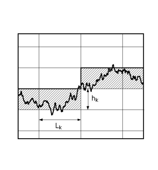
FIG. 1.: Covering procedure of a particular microscopic surface with cells of size $L_{k}\times h_{k}$. Blocks below (above) the surface are considered to be occupied (empty).

FIG. 2.: Growth rates for the KPZ dynamics in a typical configuration.

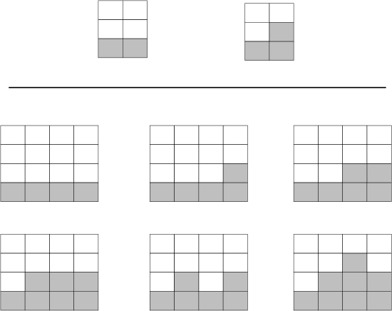
FIG. 3.: Nonequivalent surface configurations for a system of size 2 (top) and 4 (bottom) with periodic boundary conditions and $\Delta h_{max}=1$.

FIG. 4.: Results for $d=1$ and different $\Delta h_{max}$. The intersections between solid (representing the $1/2\log_{2}F_{2}(x)$) and dashed lines (representing the $1/2\log_{2}[F_{4}(x)/F_{2}(x)]$) give $x^{*}$ on the horizontal axis and $\alpha$ on the vertical axis (see Eq. (26)). Observe that, as $\Delta h_{max}$ is increased, the exact value $\alpha=1/2$ is rapidly approached.

FIG. 5.: Value of $\alpha$ as a function of the dimension obtained by the application of the method with small $b$, compared with numerical data by Ala Nissila et al. The best fit to the RG values gives slope $-0.7$. We expect this exponent to converge to $-1$ for large dimensions.

FIG. 6.: Behavior of the curves $\alpha_{b}(x)$ in $d=1$ (see Eq. (44) and (45)).

FIG. 7.: Plot of the RG estimate for the roughness exponent $\alpha$ as a function of the inverse system size. Empty symbols are for data obtained with periodic boundary conditions. Full symbols refer to open boundaries.

FIG. 8.: Value of the fixed point parameter $x^{*}$ as a function of the inverse system size. Empty symbols are for data obtained with periodic boundary conditions. Full symbols refer to open boundaries.

FIG. 9.: Value of the exponent $\alpha$ computed using the parametrization Eq. (48) for the KPZ dynamics for various values of $\gamma$ in $d=2$ and $d=4$.

FIG. 10.: Value of the exponent $\alpha$ computed using the parametrization Eq. (49) for KPZ dynamics for various values of $\gamma$ in $d=2$ and $d=4$.

FIG. 11.: Representation of a surface configuration with 8 “high” sites and $b^{d}-8$ “low”sites.

FIG. 12.: Comparison of the form of the function $\Omega_{n}$ computed with $x=0$, used in the analytical calculation (solid line), with the function determined numerically in $d=7$ for $x=\infty$ (dashed line). For intermediate values of $x$, the function $\Omega_{n}$ lies between the two curves plotted.

FIG. 13.: Plot of the left and right hand sides of Eq. (22) as computed numerically in $d=7$ and analytically (Eq. (59)).

FIG. 14.: Comparison of the dependence of $\alpha$ on $d$ computed with the RG in the large-$d$ limit Eq. (61) with the numerical data of Ala-Nissila et al.. In the inset, plot of the value of the fixed point parameter $x^{*}$ computed numerically for small $d$ and compared with the analytical expression Eq. (60).

FIG. 15.: Plot of the RG estimate for the roughness exponent $\alpha$ as a function of the inverse system size for the Edwards-Wilkinson dynamics.

$d$	1	2	3	4	5	6	7	8	9
$x^{*}$	0.726	2.77	6.96	15.91	31.96	63.5	124.5	242	468
$\alpha_{\rm RG}$	0.507	0.363	0.294	0.238	0.206	0.182	0.164	0.149	0.137
$\alpha_{\rm num}$	0.5	0.387	0.305	0.261	0.193	0.18	0.15	-	-

TABLE I.: Values of the fixed point parameter $x^{*}$ and of the roughness exponent computed with the RG with $b=2$, compared with the numerical results of Ala-Nissila et al.

REFERENCES

- [1] B. I. Halperin and P. C. Hohenberg, Phys. Rev. B 10, 139, (1974).
- [2] J. Zinn-Justin, Quantum Field Theory and Critical Phenomena (Oxford Science, Oxford, 1989); C. J. DeDominicis, J. Physique 37, 247 (1976); H.K. Janssen, Z. Phys. B 23, 377 (1976); P. C. Martin, E. D. Siggia and H. A. Rose, Phys. Rev. A 8, 423 (1978); L. Peliti, J. Physique, 46, 1469 (1985).
- [3] M. Kardar, G. Parisi and Y. C. Zhang, Phys. Rev. Lett. 56, 889 (1986).
- [4] T. Halpin-Healy and Y.-C. Zhang, Phys. Rep. 254 (1995).
- [5] J. Krug and H. Spohn, in Solids Far From Equilibrium, ed. by C. Godrèche (Cambridge University Press, Cambridge, 1990).
- [6] A. L. Barabási, H. E. Stanley, Fractal Concepts in Surface Growth Cambridge University Press, Cambridge, 1995.
- [7] See D. Forster, D. R. Nelson and M. J. Stephen, Phys. Rev. A 16, 732 (1977).
- [8] D. A. Huse, C. L. Henley, and D. S. Fisher, Phys. Rev. Lett. 55, 2924 (1985). See also [4] and [5].
- [9] G. Grinstein, M. A. Muñoz and Y. Tu, Phys. Rev. Lett. 76, 4376, (1996). Yuhai Tu, G. Grinstein and M. A. Muñoz, Phys. Rev. Lett. 78, 274 (1997).
- [10] B. Derrida and H. Spohn, J. Stat. Phys. 51, 817 (1988); M. Mézard and G. Parisi, J. Phys. (Paris) 1, 809 (1991); M. Marsili and A. J. Bray, Phys. Rev. Lett. 76, 2750 (1996).
- [11] T. W. Burkhardt and J. M. J. van Leuwen, Real space Renormalization (Springer Heidelberg), 1982.
- [12] A. Erzan, L. Pietronero and A. Vespignani, Rev. Mod. Phys. 67, 545 (1995).
- [13] J. J. Binney, N. J. Dowrick, A. J. Fisher and M. E. J. Newman, The Theory of Critical Phenomena, Clarendon Press, Oxford, 1992.
- [14] C. Castellano, M. Marsili and L. Pietronero, Phys. Rev. Lett. 80, 4830 (1998).
- [15] C. Castellano, A. Gabrielli, M. Marsili, M. A. Muñoz, and L. Pietronero, Phys. Rev. E 58, R5209 (1998).
- [16] M. Marsili and Y.C. Zhang, Phys. Rev. E 57, 4814 (1998).
- [17] Recently the method also been used to study a two-parametric dynamics, G. Bianconi, M. A. Muñoz, A. Gabrielli and L. Pietronero, (in preparation).
- [18] C. F. Baillie at al., Phys. Rev. B 45, 10438 (1992).
- [19] E. Medina, T. Hwa and M. Kardar, Phys. Rev. A 39, 3053 (1989). M. Lässig Nucl. Phys. B 448, 559 (1995).
- [20] M. Lässig, Nucl. Phys. B 448, 559 (1995).
- [21] M. Schwarz and S.F. Edwards, Europhys. Lett. 20, 310 (1992); J-P. Bouchaud and M.E. Cates, Phys. Rev. E 47, R1455 (1993); 48, 635 (1993); J. P. Doherty et al., Phys. Rev. Lett. 72, 2041 (1994); M.A. Moore et al, Phys. Rev. Lett. 74, 4257 (1995).
- [22] M. Lässig and H. Kinzelbach, Phys. Rev. Lett. 78, 903 (1997). See also M. Lässig, J. Phys. C 10, 9905 (1998).
- [23] J. K. Bhattacharjee, J. Phys. A31, L93 (1998).
- [24] T. Halpin-Healy, Phys. Rev. A 42, 711 (1990).
- [25] M. Feigelman et al, Phys. Rev. Lett. 63, 2303 (1989).
- [26] J. Cook and B. Derrida, J. Phys. A 23, 1523 (1990).
- [27] Y. Tu, Phys. Rev. Lett. 73, 3109 (1994).
- [28] J. P. Bouchaud and A. Georges, unpublished; see also M. Marsili, J. Phys. A 29, 5405 (1996).
- [29] M. Cieplak et al. Phys. Rev. Lett. 76, 3754 (1996).
- [30] T. Ala-Nissila, et al, J. Stat. Phys. 72, 207 (1993); L. H. Tang, et al, Phys. Rev. A 45, 7162 (1992); T. Ala-Nissila, Phys. Rev. Lett. 80, 887 (1998); J. M. Kim ibid 888.
- [31] C. H. Lam and F. G. Shin, Phys. Rev. E 58, 5592 (1998); T. J. Newman and M. R. Swift, Phys. Rev. Lett. 79, 2261 (1997); H. Chaté, Q-H. Chen, and L-H. Tang, Phys. Rev. Lett 81, 5471 (1998); T. J. Newman and M. R. Swift, Phys. Rev. Lett. 81, 5472 (1998);
- [32] T. J. Newman and A. J. Bray, J. Phys. A 29, 7917 (1996).
- [33] R. Livi and A. Maritan, Phys. Rev. D 23, 2252 (1981).
- [34] B. Derrida and J. Vannimenus, J. Physique Lett. 41, 473 (1980).