Theory of Dephasing by External Perturbation in Open Quantum Dots

Abstract

We propose a random matrix theory describing the influence of a time dependent external field on the average magnetoresistance of open quantum dots. The effect is taken into account in all orders of perturbation theory, and the result is applicable to both weak and strong external fields.

It is well established that the anomalous magnetoresistance of bulk disordered systems is governed by the weak localization (WL) [1, 2, 3]. Being an interference phenomenon, the WL is extremely sensitive to inelastic processes which are commonly referred to as dephasing.

Recently, another object for the studying the quantum effects appeared – ballistic quantum dots[4]. In the absence of inelastic processes, the transport properties of the dots are well described within the Random Matrix Theory (RMT)[5]. The magnetoresistance within this theory manifests itself as a crossover between two universal ensembles (orthogonal and unitary), and the strength of the magnetic field defines a position on that crossover. This approach per se does not include dephasing, and the dephasing processes were considered on a phenomenological basis [6]. The relation of this phenomenological description used to fit the data of Ref.[7] to microscopic mechanisms of dephasing is still an open question.

In this Letter, we propose a Random Matrix - like theory of the magnetoresistance affected by an external time dependent perturbation. We will be able to find both the amplitude and frequency dependence of the magnetoresistance using only one unknown parameter. This parameter can be related to the correlator of the level velocities due to the same perturbation at zero frequency and, thus, in principle can be determined by an independent experiment. After the strength of the potential is normalized by this parameter, all the results become universal. From the experimental point of view, we have in mind changing shape of a quantum dot by applying an external ac- bias.

Before we proceed, let us mention that the effect studied in the present paper is similar to that of Ref. [8], where it was shown that uniform ac- electric filed suppresses the weak localization correction to the conductivity of a disordered wire (experimentally it was studied in Ref. [9]). However the results of [8] are not directly applicable to the quantum dots with size $L$ so small that the Thouless energy $E_{T}\sim\hbar/\tau_{erg}$ is much greater than other energy scales (such as the dephasing or escape rates) of the problem (here $\tau_{erg}$ is the characteristic time for the classical particle to cover all of the available phase space).

On the other hand in this limit one can use the RMT to study the conductance of the system, see [10]. All corrections to the RMT are small as $N_{ch}/g_{dot}$; $g_{dot}=E_{T}/\delta_{1}$ and $\delta_{1}$ is the mean level spacing. We consider the WL correction to the conductance of quantum dots with the large number $N_{ch}$ of open channels. In this approximation we neglect the effect of interaction on the conductance which are small as $1/N_{ch}^{2}$[11], while the weak localization correction to the conductance is proportional to $1/N_{ch}$. The same condition also allows us to use conventional diagrammatic technique[12] to perform the ensemble average.

In general, the Hamiltonian of the system can be represented as, see [10]:

$$\hat{H}=\hat{H}_{D}+\hat{H}_{L}+\hat{H}_{LD},$$ (1)

where $\hat{H}_{D}$ is the Hamiltonian of electrons in the dot, which is determined by $M\times M$ matrix

$$\hat{H}_{D}=\sum_{n,m=1}^{M}\psi^{\dagger}_{n}H_{nm}\psi_{m},$$ (2)

where the thermodynamic limit $M\to\infty$ is assumed. We consider the case, when $H_{nm}$ is a time dependent random matrix in the form:

$$H_{nm}(t)={\cal H}_{nm}+V_{nm}\varphi(t).$$ (3)

Here the time independent part of the Hamiltonian ${\cal H}_{nm}$ is a random realization of $M\times M$ matrix, which obeys the correlation function

$$\langle{\cal H}_{nm}{\cal H}^{*}_{n^{\prime}m^{\prime}}\rangle=\lambda\delta_{nn^{\prime}}\delta_{mm^{\prime}}+\lambda^{\prime}\delta_{mn^{\prime}}\delta_{nm^{\prime}},$$ (4)

where $\lambda=M(\delta_{1}/\pi)^{2}$ and $\lambda^{\prime}=\lambda(1-g_{h}/4M)$, $g_{h}$ defines crossover from the orthogonal ($g_{h}=0$) to the unitary ($g_{h}=4M$) ensemble. Parameter $g_{h}$ has a meaning of the dephasing rate by the external magnetic field in units of the level spacing $\delta_{1}$, see [3, 10]. It can be estimated as $g_{h}\simeq g_{dot}\left(\Phi/\Phi_{0}\right)^{2}$ where $\Phi$ is the magnetic flux through the dot and $\Phi_{0}=hc/e$ is the flux quantum. The time dependent perturbation is described by symmetric $M\times M$ matrices $V_{nm}$ and a function of time $\varphi(t)$.

The coupling between the dot and the leads is

$$\hat{H}_{LD}=\sum_{\alpha,n,k}\left(W_{n\alpha}\psi^{\dagger}_{\alpha}(k)\psi_{n}+{\rm H.c.}\right),$$ (5)

where $\psi_{n}$ correspond to the states of the dot, $\psi_{\alpha}(k)$ denotes different electron states in the leads, and momentum $k$ labels continuous state in each channel $\alpha$. For the dot connected with two leads by $N_{l}$ and $N_{r}$ channels respectively, we denote the left lead channels by $1\leq\alpha\leq N_{l}$ and the right channels by $N_{l}+1\leq\alpha\leq N_{ch}$, where $N_{ch}=N_{l}+N_{r}$. The electron spectrum in the leads near Fermi surface can be linearized:

$$\hat{H}_{L}=v_{F}\sum_{\alpha,k}k\psi^{\dagger}_{\alpha}(k)\psi_{\alpha}(k),$$ (6)

where $v_{F}=1/2\pi\nu$ is the Fermi velocity and $\nu$ is the density of states at the Fermi surface.

The coupling constants $W_{n\alpha}$ in Eq.(5)are defined as[10]:

$$W_{n\alpha}=\sqrt{\frac{M\delta_{1}}{\pi^{2}\nu}}\cases{t_{\alpha},&if $n=\alpha\leq N_{ch}$,\cr`0,&otherwise,}$$ (7)

where $t_{\alpha}$ determines the dimensionless conductance of each lead (in units of $2e^{2}/h$) according to

$$\begin{array}[]{ccc}\displaystyle g_{l}=\sum_{\alpha=1}^{N_{l}}\frac{4t_{\alpha}t^{*}_{\alpha}}{(1+t_{\alpha}t^{*}_{\alpha})^{2}},&&\displaystyle g_{r}=\sum_{\alpha=N_{l}+1}^{N_{ch}}\frac{4t_{\alpha}t^{*}_{\alpha}}{(1+t_{\alpha}t^{*}_{\alpha})^{2}}\end{array}$$ (8)

and $|t_{\alpha}|\leq 1$. The factor in Eq. (7) is chosen so that the ensemble average scattering matrix ${\cal S}_{\alpha\beta}$ of a dot with fully open channels ($t_{\alpha}=1$) is zero. More complicated structure of $\hat{W}$ can be always reduced to the form (7) by suitable rotations.

For the system described above the scattering matrix $\hat{\cal S}$ has the form:

$${\cal S}_{\alpha\beta}(t,t^{\prime})=1-2\pi i\nu W^{\dagger}_{\alpha n}G_{nm}(t,t^{\prime})W_{m\beta},$$ (9)

and the Green’s function $G_{nm}(t,t^{\prime})$ is the solution to:

$$\left(i\frac{\partial}{\partial t}-{\hat{H}}(t)+i\pi\nu\hat{W}\hat{W}^{\dagger}\right)\hat{G}(t,t^{\prime})=\delta(t-t^{\prime}),$$ (10)

where matrices $\hat{H}$ and $\hat{W}$ are comprised by their elements (3) and (7) respectively.

The averaged dimensionless $dc$ - conductance of the dot is determined in terms of the scattering matrix of the system in the linear response theory by (see, e.g. [10]):

$$g={\Big{\langle}}\int_{-\infty}^{t}dt^{\prime}{\mathrm{t}r}\left[\hat{\tau}_{l}{\cal S}(t,t^{\prime})\hat{\tau}_{r}{\cal S}^{\dagger}(t,t^{\prime})\right]{\Big{\rangle}},$$ (11)

where $\langle\dots\rangle$ stands for both ensemble and time averages. We also introduced notation for the projector on the left lead, $\hat{\tau}_{l}$, which is a diagonal $N_{ch}\times N_{ch}$ matrix with the first $N_{l}$ diagonal elements equal to unity, and the other diagonal elements equal to zero, and $\hat{\tau}_{r}=\hat{I}-\hat{\tau}_{l}$.

We perform calculations of the average conductance keeping the leading terms in $1/M$. The diagrammatic technique is somewhat similar to that developed for bulk metals [12], where the small parameter is $1/\epsilon_{F}\tau_{imp}$ with $\epsilon_{F}$ being the Fermi energy and $\tau_{imp}$ being the elastic mean free time.

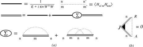
FIG. 1.: (a) Diagrams for the ensemble average Green’s function. The second term in the self-energy includes an intersection of dashed lines and it is small as $1/M$. (b) The representation of the conductance in the form of Eq. (13) forbids the renormalization of vertices $J$ from Eq. (15) by disorder.

First let us find the ensemble average Green’s function $\langle G^{(R)}\rangle$. One can see that $\langle G^{(R)}\rangle$ is diagonal, $\langle G^{(R)}_{nm}(\epsilon)\rangle=\delta_{nm}G^{(R)}_{n}(\epsilon)$ Using the self consistency equation for the Green’s function, Fig. 1 (a), we find

$$G^{(R)}_{n}(\epsilon)=\frac{1}{i\sqrt{\lambda M}}\cases{\displaystyle\frac{1}{1+t_{n}t_{n}^{*}},&$n\leq N_{ch}$,\cr\displaystyle 1+\frac{\sum_{\alpha=1}^{N_{ch}}\frac{2t_{\alpha}t_{\alpha}^{*}}{1+t_{\alpha}t_{\alpha}^{*}}+i\epsilon}{4M},&$n>N_{ch}$.}$$ (12)

Here we introduced the dimensionless energy $\epsilon$ measured in units of $\sqrt{\lambda/4M}=\delta_{1}/2\pi$. We expand these Green’s functions in $\epsilon/M$ and $(g_{l}+g_{r})/M$, since only those terms survive the thermodynamic limit $M\to\infty$. For the same reason, the expression for $G^{(R)}_{n}$ with $n\leq N_{ch}$ neglects such terms at all because the contribution of those elements to the final answer is already small as $N_{ch}/M$.

To simplify further manipulations, we rearrange Eq. (11) in the following form

$$\displaystyle g(t) = {\Big{\langle}}\int\limits_{-\infty}^{t}dt^{\prime}{\rm tr}\left[\hat{J}_{l}{\cal S}(t,t^{\prime})\hat{J}_{r}{\cal S}^{\dagger}(t,t^{\prime})\right]{\Big{\rangle}}$$ (13)

$$+ \frac{N_{r}g_{l}^{2}+N_{l}g_{r}^{2}}{(g_{l}+g_{r})^{2}},$$ (14)

$$\hat{J}_{l,r} = \hat{\tau}_{l,r}-\frac{g_{l,r}}{g_{l}+g_{r}}\hat{I}.$$ (15)

Equation (13) immediately follows from Eq. (11) and the unitarity of the ${\cal S}$- matrix ${\cal S}{\cal S}^{\dagger}=1$. The calculations of the conductance in the form of Eq. (13) are significantly simpler since the vertices (15) are not dressed by dashed lines, see Fig. 1(b). This trick is similar to the calculation of the conductivity of disordered bulk systems in terms of the current-current instead of density-density correlation function, see Refs. [2, 3].

Now we substitute the scattering matrix defined by Eq. (9) to Eq. (13). To the leading order in $1/(g_{l}+g_{r})$ one can average ${\cal S}$ -matrices independently with the help of Eq. (12) and obtain the classical conductance

$$g_{cl}=\frac{g_{l}g_{r}}{g_{l}+g_{r}}.$$ (16)

In particular, for the dot with fully open channels ($t_{\alpha}=1$), the averaged ${\cal S}$- matrix vanishes ($\langle{\cal S}\rangle=0$) and the last term of Eq. (13) gives the known result $g_{cl}=N_{l}N_{r}/N_{ch}$, since in this case $g_{l,r}=N_{l,r}$.

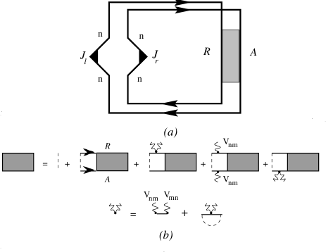
FIG. 2.: (a) The diagram for the WL correction to the conductance. (b) The diagram equation for the Cooperon.

The first order correction in $1/(g_{l}+g_{r})$ to Eq. (16) is given by the diagram in Fig. 2(a). It represents the WL correction to the conductance, and has the analytic expression

$$\Delta g_{wl}=-\frac{f_{l}g_{r}^{2}+f_{r}g^{2}_{l}}{(g_{l}+g_{r})^{2}}\int\limits_{0}^{2\pi/\omega}\!\frac{\omega dT}{2\pi}\int\limits_{0}^{\infty}\!2d\tau{\cal C}(T,\tau,-\tau),$$ (17)

where formfactors $f_{l,r}$ are given by

$$\begin{array}[]{lr}\displaystyle f_{l}=\sum_{\alpha=1}^{N_{l}}\frac{16(t_{\alpha}t^{*}_{\alpha})^{2}}{(1+t_{\alpha}t^{*}_{\alpha})^{4}},&\displaystyle f_{r}=\sum_{\alpha=N_{l}+1}^{N_{ch}}\frac{16(t_{\alpha}t^{*}_{\alpha})^{2}}{(1+t_{\alpha}t^{*}_{\alpha})^{4}}.\end{array}$$ (18)

The Cooperon ${\cal C}$ is defined by Fig. 2(b):

$$\left(\frac{\partial}{\partial\tau}+{\cal K}(T,\tau)\right){\cal C}(T,\tau,\tau^{\prime})=\delta(\tau-\tau^{\prime}),$$ (19)

where time is measured in units of inverse level spacing $2\pi/\delta_{1}$ and the “Hamiltonian” for the Cooperon is

$${\cal K}(T,\tau)=g_{*}+\pi^{2}C_{0}\left[\varphi(T+\tau/2)-\varphi(T-\tau/2)\right]^{2},$$ (20)

with $g_{*}$ characterizes the total dephasing due to the escape and the magnetic field, $g_{*}=g_{l}+g_{r}+g_{h}$, and we chose $\varphi(t)=\cos\omega t$ to describe the time dependence of the perturbation.

The only unknown parameter, $C_{0}$, in Eq. (20) depends on the strength of the perturbation. In terms of the original Hamiltonian (3), it is defined as

$${C}_{0}=\frac{2}{\pi^{2}M\lambda}\sum_{nm}V^{2}_{nm},$$ (21)

where we used the fact that the matrix $\hat{V}$ is symmetric. This parameter is also related to the typical value of the level velocities, which characterizes the evolution of energy levels $\epsilon_{\nu}(X)$ under the action of the external perturbation $X\hat{V}$, see [13]:

$$\delta_{1}^{2}C_{0}={\Big{\langle}}\left(\frac{\partial\epsilon_{\nu}}{\partial X}\right)^{2}{\Big{\rangle}}-{\Big{\langle}}\frac{\partial\epsilon_{\nu}}{\partial X}{\Big{\rangle}}^{2}.$$ (22)

Since all other responses (e.g. parametric dependence of the conductance of the dot) are expressed in terms of universal functions of the same parameter $C_{0}$ [13], it can be found from independent measurements. For not very realistic case of homogeneous electric field $E$ introduced into the dot of linear size $L$, one can estimate $C_{0}\simeq(eEL)^{2}/(E_{T}\delta_{1})$. It is important to emphasize that the homogeneous shift of all levels does not affect the magnetoresistance and that is why the average level velocity $\langle\partial\epsilon_{\nu}/\partial X\rangle$ is not relevant.

In the absence of the time dependent perturbation $\varphi\equiv 0$, one obtains [10, 14] from Eqs. (17)–(20):

$$\Delta g_{wl}^{(0)}=-\frac{f_{l}g_{r}^{2}+f_{r}g^{2}_{l}}{(g_{l}+g_{r})^{2}g_{*}}.$$ (23)

The solution to Eq. (19) gives the weak localization correction to the conductance $\Delta g_{wl}$ in the presence of the time dependent field. It can be expressed in terms of the unperturbed correction (23) as

$$\frac{\Delta g_{wl}}{\Delta g^{(0)}_{wl}}=F\left(y,z\right),\quad y=\frac{\pi\omega}{g_{*}\delta_{1}},\ z=\frac{\pi^{2}C_{0}}{g_{*}},$$ (24)

where dimensionless function $F(y,z)$ is given by

$$F(y,z)=\!\int_{0}^{\infty}\!dxe^{-x-z\phi}{\mathrm{I}}_{0}\left[z\phi\right],\quad\phi=x-\frac{\sin xy}{y}.$$ (25)

Here ${\mathrm{I}}_{0}(\xi)$ is the modified Bessel function. Some curves for this function are plotted in Fig. 3.

Equations (24) – (25) are the main results of our paper. They give the universal description of the effect of the external field on the weak localization correction. Below we will discuss different asymptotic regimes and compare them with the results for bulk systems [3].

For weak external field $z\ll{\mathrm{m}ax}(1,y^{-2})$ we find

$$\frac{\Delta g_{wl}}{\Delta g^{(0)}_{wl}}=1-\frac{\pi^{2}C_{0}}{g_{*}}\frac{\pi^{2}\omega^{2}}{\pi^{2}\omega^{2}+\delta_{1}^{2}g_{*}^{2}}.$$ (26)

In this regime the correction is quadratic in the frequency for slowly oscillating field, similarly to the bulk system result at $\omega$ smaller than the dephasing rate $1/\tau_{\phi}$. However, the frequency dependence saturates at large frequency. It is different from the result for bulk systems, where a characteristic spatial scale shrinks as $1/\sqrt{\omega}$, whereas in our case it is determined by the size of the dot.

FIG. 3.: Representative curves of $F(y,z)$ as a function of $z$ for two values of $y$. It decreases linearly with $z$ at small values of $z$. The inset shows the $y-$dependence of the function $F(y,z)$ for two values of $z$. It decreases quadratically in $y$ at small values of $y$ and saturates at larger $y$.

In the opposite limit of strong external field $z\gg{\mathrm{m}ax}(1,y^{-2})$ we have to consider separately the cases of fast, $y\gg 1$, and slow, $y\ll 1$ field oscillations. In the first case we find

$$\frac{\Delta g_{wl}}{\Delta g^{(0)}_{wl}}=\sqrt{\frac{g_{*}}{2\pi^{2}C_{0}}}.$$ (27)

The linear dependence of the quantum correction on $1/\sqrt{C_{0}}$ is similar to that for the bulk system. Contrary to the bulk systems, the result does not depend on the frequency $\omega$ for reasons we have already discussed.

In the case of slow field $y\ll 1$, but still $zy^{2}\gg 1$ (strong field) we obtain

$$\frac{\Delta g_{wl}}{\Delta g^{(0)}_{wl}}=\frac{\Gamma(1/6)}{\pi\Gamma(5/6)}\left(\frac{2\delta_{1}^{2}g_{*}^{3}}{9C_{0}\omega^{2}}\right)^{1/3},$$ (28)

i.e., the dependences both on the amplitude and frequency are different from the bulk case.

In conclusion, we proposed a random matrix theory describing influence of time dependent external field on the average magnetoresistance of open quantum dots. This dependence can be recast in the form of the universal function Eq.(25) of one fitting parameter Eq.(22) which can be fixed by an independent experiment. The results can not be described by a simple replacement $g_{\ast}\to g_{\ast}+\gamma_{\phi}$. Finally, we mention that thermal fluctuations of the gate potentials may induce the dephasing by virtue of the mechanism considered here. However, the spectral density of such fluctuations is model dependent which makes quantitative predictions hardly possible.

We acknowledge discussions with B.L. Altshuler, V. Ambegaokar, and C.M. Marcus. Work was supported by Cornell Center for Materials Research, funded under NSF grant DMR-9632275 (MGV), and A.P. Sloan and Packard foundations (ILA).

REFERENCES

- [1] B.L. Altshuler et. al., Phys. Rev. B 22, 5142 (1980); S. Hikami, A.I. Larkin, and Y. Nagaoka, Progr. Theor. Phys. 63, 707 (1980).
- [2] B.L. Altshuler and A.G. Aronov, in Electron-Electron Interactions in Disordered Ststems, eds. A.L. Efros, M. Pollak (North-Holland, Amserdam, 1985).
- [3] B.L. Altshuler, et. al., in Quantum Theory of Solids, (Mir, Moscow, 1982).
- [4] See L.P. Kouwenhoven et. al. Proceedings of the Advanced Study Institute on Mesoscopic Electron Transport, Eds. L. Sohn, L.P. Kouwenhoven and G. Schoen (Kluwer, Series E, 1997) for the review.
- [5] H.U. Baranger and P.A. Mello, Phys. Rev. Lett., 73, 142, (1994); R.A. Jalabert, J.L. Pichard, C.W.J. Beenakker, Europhys. Lett, 27, 255, (1994) see Ref. [10].
- [6] H.U. Baranger, P.A. Mello, Phys. Rev. B, 51, 4703, (1995); P.W. Brouwer and C.W.J. Beenakker, ibid., 51, 7739, (1995); ibid., 55, 4695, (1997); I.L. Aleiner and A.I. Larkin. ibid., 54, 14423 (1996); E. McCann and I.V. Lerner, ibid., 57, 7219 (1998).
- [7] A.G. Huibers et. al., Phys. Rev. Lett., 81, 200 (1998); cond-mat/9904274.
- [8] B.L. Altshuler, A.G. Aronov, and D.E. Khmelnitskii, Solid State Commun., 39, 619, (1981).
- [9] S.A. Vitkalov et. al., JETP Lett., 43, 185, (1986); Sov. Phys. JETP, 67, 1080, (1988).
- [10] C.W.J. Beenakker, Rev. Mod. Phys, 69, 731, (1997).
- [11] P.W. Brouwer and I.L. Aleiner, Phys. Rev. Lett., 82, 390 (1999).
- [12] A.A. Abrikosov, L.P. Gorkov, I.E. Dzyaloshinskii, Methods of Quantum Field Theory in Statistical Physics, (Prentice–Hall, Englewood Cliffs, NJ, 1963).
- [13] B.D. Simons and B.L. Altshuler, Phys. Rev. Lett., 70, 4063, (1993); B.L. Altshuler and B.D. Simons, in Mesoscopic Quantum Physics, eds. E. Akkermans et. al, (Elsevier, 1995).
- [14] P.W. Brouwer and C.W.J. Beenakker, J. Math. Phys., 37, 4904 (1996).