Spin-Gap Phases in Tomonaga-Luttinger Liquids

Abstract

We give the details of the analysis for critical properties of spin-gap phases in one-dimensional lattice electron models. In the Tomonaga-Luttinger (TL) liquid theory, the spin-gap instability occurs when the backward scattering changes from repulsive to attractive. This transition point is shown to be equivalent to that of the level-crossing of the singlet and the triplet excitation spectra, using the $c=1$ conformal field theory and the renormalization group. Based on this notion, the transition point between the TL liquid and the spin-gap phases can be determined with high-accuracy from the numerical data of finite-size clusters. We also discuss the boundary conditions and discrete symmetries to extract these excitation spectra. This technique is applied to the extended Hubbard model, the $t$-$J$ model, and the $t$-$J$-$J^{\prime}$ model, and their phase diagrams are obtained. We also discuss the relation between our results and analytical solutions in weak-coupling and low-density limits.

]

I Introduction

Spin-gap phases of one-dimensional (1D) electron systems have been studied for long times. This research has been motivated by the phase transitions in 1D organic conductors. In the past decade, the discovery of high-$T_{\rm c}$ superconductivity strongly stimulated this study.

The spin-gap transition in 1D lattice models had been mainly analyzed by two approaches: The one is the weak coupling theory based on the bosonization theory and renormalization group. The other is numerical calculation in finite-size systems which is free from approximation. In the former scheme, the existence of the gap is argued by investigating the backward scattering effect on the fixed point, but the validity of the result is ensured only in the weak coupling limit. On the other hand, in numerical calculation, the analysis is done by a direct evaluation of the gap and the finite-size scaling method. In this approach, a singular behavior of the gap near the critical point makes it difficult to make out the instability.

In order to illustrate the difficulty in the determination of the phase boundary, let us consider the Hubbard model,

$${\cal H}_{\rm HM}=-t\sum_{is}(c^{{\dagger}}_{is}c_{i+1,s}+\mbox{H.c})+U\sum_{i}n_{i\uparrow}n_{i\downarrow}.$$ (1)

This model has a spin gap for $U<0$. According to the Bethe-ansatz result for the charge gap at half-filling[4] combining a canonical transformation [5], we can obtain the asymptotic behavior of the spin gap near the critical point $U=0$ as

$$\Delta E\sim\sqrt{2t|U|}{\rm e}^{-\pi t/|U|}.$$ (2)

Since the gap opens slowly near the critical point, it is very difficult to find the critical point using conventional finite-size scaling method.

In this paper, we give a remedy for this problem[6, 7]. The many-body problem is often simplified by using the notion of universality. Generally, 1D electron systems belong to the universality class of Tomonaga-Luttinger (TL) liquids[8, 9, 10, 11, 12] which are characterized by gapless charge and spin excitations and power-law decay of correlation functions. This behavior can be described by the bosonization theory or the $c=1$ conformal field theory (CFT). In this scheme, the phase transition to the spin-gap phase is understood as an instability caused by the backward scattering process using the renormalization group technique[13], and a spin gap opens when the backward scattering turns from repulsive to attractive. This transition point is equivalent to the level-crossing of the singlet-triplet excitation spectra[14, 15, 16], by taking account of the logarithmic corrections originated from the backward scattering.

In this paper, we will analyze the following models based on this notion. The first example is the extended Hubbard model which is given by

$${\cal H}_{\rm EHM}={\cal H}_{\rm HM}+V\sum_{i}n_{i}n_{i+1}.$$ (3)

For the study of spin-gap transitions, this model has been analyzed by the g-ology for weak coupling region[10, 11]. The numerical calculation was performed by the exact diagonalization with finite-size scaling method[17, 18, 19]. However, the spin-gap phase boundary has not been clarified.

The next example is the $t$-$J$ model described by

$${\cal H}_{t\mbox{-}J} = -t\sum_{is}(\tilde{c}^{{\dagger}}_{is}\tilde{c}_{i+1,s}+\mbox{H.c.})$$ (5)

$$+J\sum_{i}(\mbox{\boldmath$S$}_{i}\cdot\mbox{\boldmath$S$}_{i+1}-n_{i}n_{i+1}/4),$$

where $\tilde{c}_{is}=c_{is}(1-n_{i,-s})$. This model is obtained by doping holes in the Heisenberg spin chain. For this model, the weak coupling treatment is difficult due to this strong coupling constraint, however, the universality class of this model is known as TL liquids, from the analysis for the exactly solvable cases at $J/t=0$ (spinless fermion) and $J/t=2$ (super-symmetric point)[20, 21]. The remaining region was analyzed using the exact diagonalization by Ogata et al.[22]. Their phase diagram shows the enhancement of the superconducting correlation ($K_{\rho}>1$) and the phase separation ($K_{\rho}\rightarrow\infty$) for the large $J/t$ region. According to their result, the spin-gap phase does not exist except for the low density region. Variational approaches also played roles in the analysis for this model[23, 24, 25], but could not establish clear solution for the spin-gap phase.

Extensions of the $t$-$J$ model are also considered by many researchers [26, 27, 28, 29, 30, 31]. In spin systems, a spin gap opens by the effect of frustration or dimerization. Metallic spin-gap phases can be generated by doping holes in these spin systems. In this paper, we concentrate our attention on the $t$-$J$-$J^{\prime}$ model which includes the effect of frustration[26, 27]:

$${\cal H}_{t\mbox{-}J\mbox{-}J^{\prime}} = {\cal H}_{t\mbox{-}J}+J^{\prime}\sum_{i}(\mbox{\boldmath$S$}_{i}\cdot\mbox{\boldmath$S$}_{i+2}-n_{i}n_{i+2}/4).$$ (6)

We introduce a parameter $\alpha$ for the strength of the frustration given by $\alpha\equiv J^{\prime}/J$. At half-filling ($n=1$), this model becomes an $S=1/2$ frustrated spin chain. In this case, the ground state at $\alpha=1/2$ is the two-fold degenerate dimer state with a spin gap, and the ground state energy density is $-3/4J$[32, 33, 34]. The fluid-dimer transition occurs at $\alpha_{\rm c}=0.2411$[16]. Upon doping of holes, the system may become metallic, and the spin gap is reduced[26] but persists for the finite doping. The phase diagram of this model for $n\neq 1$ at $\alpha=1/2$, using the exact diagonalization, was obtained by Ogata, Luchini, and Rice[27], but the phase boundary of the spin-gap phase was also remained to be ambiguous.

This paper is organized as follows. In Sec.II, we discuss, based on the continuum field theory, that the level crossing of singlet and triplet excitation spectra gives the critical point of the spin-gap transition. In Sec.III, we consider boundary conditions for the unique ground state, and discrete symmetries of wave functions to identify the energy spectra observed in our analysis. In Sec.IV, we analyze representative models introduced above, and clarify the spin-gap region in the phase diagrams, and check the consistency of our argument. Finally, in Sec.V, we present our conclusions.

The paper also contains three Appendices. The first shows the relation among the different notations for the quantum numbers. The second is derivation for the logarithmic corrections. The third explains the calculation in two-electron systems.

II Continuum Field Theory

A Effective Hamiltonian

Let us start our argument from the Abelian bosonization theory of electrons[9, 10, 11, 12, 35]. The low-energy excitations are described by continuous fermion fields which are defined by

$$c_{j,s}\rightarrow\psi_{{\rm L},s}(x)+\psi_{{\rm R},s}(x)$$ (7)

The boson representation of the fermion operator is

$$\psi_{r,s}(x)=\frac{1}{\sqrt{2\pi\alpha}}{\rm e}^{{\rm i}rk_{\rm F}x}{\rm e}^{{\rm i}/\sqrt{2}\cdot[r(\phi_{\rho}+s\phi_{\sigma})-\theta_{\rho}-s\theta_{\sigma}]},$$ (8)

where $\alpha$ is a short-distance cutoff. $r={\rm R},{\rm L}$ and $s=\uparrow,\downarrow$ refer to $+,-$ in that order. The phase fields are defined as

$$\phi_{\nu}(x) = -\frac{{\rm i}\pi}{L}\sum_{p\neq 0}A_{p}(x)\left[\nu_{\rm R}(p)+\nu_{\rm L}(p)\right]-\frac{\sqrt{2}\pi x}{L}\hat{n}_{\nu},$$ (10)

$$\theta_{\nu}(x) = +\frac{{\rm i}\pi}{L}\sum_{p\neq 0}A_{p}(x)\left[\nu_{\rm R}(p)-\nu_{\rm L}(p)\right]+\frac{\sqrt{2}\pi x}{L}\hat{m}_{\nu},$$ (11)

where $A_{p}(x)\equiv\frac{1}{p}{\rm e}^{-{\rm i}\alpha|p|/2-{\rm i}px}$, and $\nu_{r}$ is the charge ($\nu=\rho$) or the spin ($\nu=\sigma$) density operator. These phase fields satisfy the relation $\left[\phi_{\nu}(x),\theta_{\nu}(x^{\prime})\right]=-{\rm i}\pi{\rm\,sign}(x-x^{\prime})/2$.

Using above relations, effective Hamiltonian of a 1D electron system is described by the U(1) Gaussian model (charge part) and the SU(2) sine-Gordon model (spin part),

$${\cal H}={\cal H}_{\rho}+{\cal H}_{\sigma}+\frac{2g_{1\perp}}{(2\pi\alpha)^{2}}\int_{0}^{L}{\rm d}x\cos(\sqrt{8}\phi_{\sigma}).$$ (12)

Here $g_{1\perp}$ is the backward scattering amplitude and for $\nu=\rho,\sigma$

$${\cal H}_{\nu}=\frac{v_{\nu}}{2\pi}\int_{0}^{L}{\rm d}x\left[K_{\nu}(\partial_{x}\theta_{\nu})^{2}+K_{\nu}^{-1}(\partial_{x}\phi_{\nu})^{2}\right],$$ (13)

where $v_{\nu}$ and $K_{\nu}$ are the velocity and the Gaussian coupling, respectively, for the charge ($\nu=\rho$) and the spin ($\nu=\sigma$) sectors. In the TL phase ($g_{1\perp}>0$), the parameters $K_{\sigma}$ and $g_{1\perp}$ are renormalized as $K^{*}_{\sigma}=1$ and $g_{1\perp}^{*}=0$, reflecting the SU(2) symmetry.

The phase fields defined in eqs.(8) satisfy the following boundary conditions,

$$\phi_{\nu}(x+L) = \phi_{\nu}(x)-\sqrt{2}\pi n_{\nu},$$ (15)

$$\theta_{\nu}(x+L) = \theta_{\nu}(x)+\sqrt{2}\pi m_{\nu}.$$ (16)

The quantum numbers $m_{\nu}$ and $n_{\nu}$ are defined by the eigen values of the total number operators $\hat{N}_{r,s}$ (measured with respect to the ground state) for right and left going particles ($r={\rm R},{\rm L}$) of spin $s$

$$n_{\nu} = [(N_{{\rm R}\uparrow}+N_{{\rm L}\uparrow})\pm(N_{{\rm R}\downarrow}+N_{{\rm L}\downarrow})]/2,$$ (18)

$$m_{\nu} = [(N_{{\rm R}\uparrow}-N_{{\rm L}\uparrow})\pm(N_{{\rm R}\downarrow}-N_{{\rm L}\downarrow})]/2.$$ (19)

Here the upper and lower sign refer to charge ($\nu=\rho$) and spin ($\nu=\sigma$) degrees of freedoms, respectively. Thus $n_{\nu}$ denotes excitations involving the variation of particles numbers and $m_{\nu}$ indicate current excitations. If we require $N_{r,s}$ to be an integer, the possible value of the quantum numbers are restricted as

$$(-1)^{m_{\rho}\pm m_{\sigma}}=(-1)^{n_{\rho}\pm n_{\sigma}}.$$ (20)

This is the selection rule for the quantum numbers[9, 38].

B Excitation Spectra and Boundary Conditions

First, we consider the excitation spectra for $g_{1\perp}=0$ case. If the system is periodic, and has unique ground state, the ground state energy of the system with length $L$ is given by[36]

$$E_{0}(L)=L\epsilon_{0}-\frac{\pi(v_{\rho}+v_{\sigma})}{6L}c,$$ (21)

where the central charge $c$ characterizes the universality class of the model. The finite-size corrections for the excitation energy and momentum of the system are described by[37, 9]

$$E-E_{0} = \frac{2\pi v_{\rho}}{L}x_{\rho}+\frac{2\pi v_{\sigma}}{L}x_{\sigma},$$ (22)

$$P-P_{0} = \frac{2\pi}{L}(s_{\rho}+s_{\sigma})+2m_{\rho}k_{\rm F},$$ (23)

where $k_{\rm F}=\pi N/2L$ is the Fermi wave number. $x_{\nu}=\Delta_{\nu}^{+}+\Delta_{\nu}^{-},s_{\nu}=\Delta_{\nu}^{+}-\Delta_{\nu}^{-}$ are the scaling dimension and the conformal spin, respectively, where the conformal weights for each sector are given by

$$\Delta_{\nu}^{\pm}=\frac{1}{2}\left(\sqrt{\frac{K_{\nu}}{2}}m_{\nu}\pm\frac{n_{\nu}}{\sqrt{2K_{\nu}}}\right)^{2}+n_{\nu}^{\pm}.$$ (24)

Here the integer $n_{\nu}^{\pm}$ denote descendant fields which describe particle-hole excitations near the Fermi points. The scaling dimensions are related to the critical exponents for the correlation functions as

$$\langle{\cal O}_{i}(r){\cal O}_{i}(r^{\prime})\rangle\sim|r-r^{\prime}|^{-2(x_{\rho i}+x_{\sigma i})}.$$ (25)

Therefore, there is one to one correspondence between the excitation spectra and the operators. The operators correspond to the excited states are given by

$${\cal O}_{m_{\rho},m_{\sigma},n_{\rho},n_{\sigma}}\propto{\rm e}^{{\rm i}\sqrt{2}(m_{\rho}\phi_{\rho}+m_{\sigma}\phi_{\sigma}+n_{\rho}\theta_{\rho}+n_{\sigma}\theta_{\sigma})},$$ (26)

or their linear combinations. From eqs.(8) and (II A), the Fermi operator takes the following boundary conditions depending on the excited states:

$$\psi_{r,s}(x+L)=\psi_{r,s}(x){\rm e}^{{\rm i}\pi(m_{\rho}+m_{\sigma}+n_{\rho}+n_{\sigma})}.$$ (27)

This means that the excited states given by arbitrary combination of quantum numbers are realized by changing the boundary conditions, while, for fixed boundary conditions, the possible excited states are restricted by the selection rule (20).

The excitation spectra on which we will turn our attention can be obtained based on the operators for the charge-density-wave (CDW) and the spin-density-wave (SDW):

$${\cal O}_{\rm CDW} = \psi^{{\dagger}}_{{\rm L}\uparrow}\psi_{{\rm R}\uparrow}+\psi^{{\dagger}}_{{\rm L}\downarrow}\psi_{{\rm R}\downarrow}$$ (29)

$$= \frac{1}{\pi\alpha}\exp({\rm i}2k_{\rm F}x+{\rm i}\sqrt{2}\phi_{\rho})\cos(\sqrt{2}\phi_{\sigma}),$$ (30)

$${\cal O}_{{\rm SDW},z} = \psi^{{\dagger}}_{{\rm L}\uparrow}\psi_{{\rm R}\uparrow}-\psi^{{\dagger}}_{{\rm L}\downarrow}\psi_{{\rm R}\downarrow}$$ (31)

$$= \frac{{\rm i}}{\pi\alpha}\exp({\rm i}2k_{\rm F}x+{\rm i}\sqrt{2}\phi_{\rho})\sin(\sqrt{2}\phi_{\sigma}),$$ (32)

$${\cal O}_{{\rm SDW},+} = \psi^{{\dagger}}_{{\rm L}\uparrow}\psi_{{\rm R}\downarrow}$$ (33)

$$= \frac{1}{2\pi\alpha}\exp({\rm i}2k_{\rm F}x+{\rm i}\sqrt{2}\phi_{\rho})\exp(+{\rm i}\sqrt{2}\theta_{\sigma}).$$ (34)

These excitation spectra consist of the charge part which carries the momentum $2k_{\rm F}$, and the spin part which forms singlet ($\sqrt{2}\cos\sqrt{2}\phi_{\sigma}$) and triplet ($\sqrt{2}\sin\sqrt{2}\phi_{\sigma},\exp(\pm{\rm i}\sqrt{2}\theta_{\sigma})$) states. Note that the spin part of the singlet and the triplet superconducting operators (SS, TS) are obtained with $k_{\rm F}=0$ and replacing $\phi_{\rho}\rightarrow\theta_{\rho}$.

If charge-spin separation occurs, the spin excitations in eqs.(II B) ($m_{\sigma}=1$ or $n_{\sigma}=1$, otherwise $=0$) can be extracted by using anti-periodic boundary conditions following eq.(27). In the continuum field theory based on the TL model, the dispersion relation is approximated by linearized one, so that the deviation from the approximated dispersion become smaller if the excitation energies become lower by eliminating the charge excitations. Therefore, the precision of the analysis is enhanced by twisting the boundary conditions.

The twisted boundary conditions are also important in identification of excitation spectra. Under anti-periodic boundary conditions, the momenta of these states are reduced to zero. Then we can define the parity transformation to classify these spectra. Although the space-inversion operator and translation operator do not commute, we can classify these spectra simultaneously by wave numbers and parities, if the wave number $k$ takes $0$ or $\pi$. From eq.(8), the phase fields $\phi_{\nu}$ change under the parity (${\cal P}$: R$\leftrightarrow$L), and the spin-reversal transformations (${\cal T}$: $\uparrow\leftrightarrow\downarrow$) as[39]

$${\cal P}: \phi_{\sigma}\rightarrow-\phi_{\sigma},\ \ \ \phi_{\rho}\rightarrow-\phi_{\rho}$$ (36)

$${\cal T}: \phi_{\sigma}\rightarrow-\phi_{\sigma}$$ (37)

Thus operators have discrete symmetries as ${\cal P}={\cal T}=1$ for the singlet ($\sqrt{2}\cos\sqrt{2}\phi_{\sigma}$), and ${\cal P}={\cal T}=-1$ for the triplet with $S^{z}=0$ ($\sqrt{2}\sin\sqrt{2}\phi_{\sigma}$). The discrete symmetries of the wave functions of these excited states are determined by combinations of those of the ground state and the operators. Further discussion for the discrete symmetries will be given in the next section.

C Renormalization Group

Next, we consider the renormalization ($g_{1\perp}\neq 0$). By the change of the cut off $\alpha\rightarrow{\rm e}^{{\rm d}l}\alpha$, the coupling constant $g_{1\perp}$ and $K_{\sigma}$ are renormalized as[40]

$$\frac{{\rm d}y_{0}(l)}{{\rm d}l} = -y_{1}^{\ 2}(l),$$ (39)

$$\frac{{\rm d}y_{1}(l)}{{\rm d}l} = -y_{0}(l)y_{1}(l),$$ (40)

where $y_{0}(l)\equiv 2(K_{\sigma}-1),y_{1}(l)\equiv g_{1\perp}/\pi v_{\sigma}$. For the SU(2) symmetric case $y_{0}(l)=y_{1}(l)$ (the level-$1$ SU(2) Wess-Zumino-Novikov-Witten (WZNW) model[41, 42, 14]) and $y_{0}(l)>0$, the scaling dimensions of the operators for singlet and triplet excitations split logarithmically by the marginally irrelevant coupling as[43, 14] (see Appendix B)

$$x_{\sigma}^{\rm singlet} = \frac{1}{2}+\frac{3}{4}\frac{y_{0}}{y_{0}\ln L+1},$$ (42)

$$x_{\sigma}^{\rm triplet} = \frac{1}{2}-\frac{1}{4}\frac{y_{0}}{y_{0}\ln L+1},$$ (43)

where $y_{0}\equiv y_{0}(0)$ and we have set $l=\ln L$. When $y_{0}<0$, $y_{0}(l)$ is renormalized to $y_{0}(l)\rightarrow-\infty$, then a spin gap appears. At the critical point ($y_{0}=0$), there are no logarithmic corrections in the excitation gaps (the logarithmic correction from higher order also vanish). Therefore, the critical point is obtained from the intersection of the singlet and the triplet excitation spectra[14, 15, 16]. In this case, we can determine the critical point with high precision[16], since the remaining correction is only $x_{\nu}=4$ irrelevant fields[44, 45]. This irrelevant field, which does not exist in the pure sine-Gordon model, comes from the nonlinear term neglected when linearizing the dispersion relation near the Fermi level in the course of the bosonization.

The physical meaning of this transition point ($y_{0}=0$) is the one where the backward scattering coupling changes from repulsive to attractive. Moreover, at the critical point, the SU(2) symmetry is enhanced to the chiral SU(2)$\times$SU(2) symmetry[14], since the spin degrees of freedom of the right and the left Fermi points become independent.

Eq.(II C) also explains the fact that the SDW (CDW) correlation is dominant for $K_{\rho}<1$ region with(out) spin gap, while for $K_{\rho}>1$, the TS (SS) correlation is dominant with(out) spin gap[43].

Finally, let us consider the massive region. The behavior of the gap is explained from the two-loop renormalization group equation of the level-1 SU(2) WZNW model[46, 47, 48]

$$\frac{{\rm d}y_{0}(l)}{{\rm d}l}=-y_{0}^{\ 2}(l)-\frac{1}{2}y_{0}^{\ 3}(l).$$ (44)

If we define the correlation length $\xi$ as $y_{0}(\ln\xi)\equiv-1$ and the energy gap as $\Delta E=v_{\sigma}/\xi$, then one can derive the asymptotic form of the spin gap by solving the differential equation for $|y_{0}(l)|\ll 1$ as

$$\Delta E\propto\sqrt{|y_{0}|}\exp(-\mbox{Const.}/|y_{0}|).$$ (45)

Note that eq.(45) is the same asymptotic behavior as the spin gap of the negative-$U$ Hubbard model at half-filling given by eq.(2).

III Uniqueness of Ground State and Discrete Symmetries

In the previous section, the ground state is assumed to be a singlet, so that we should consider the way to make the singlet ground state in the finite-size systems. Furthermore, we also discuss the discrete symmetries of wave functions to identify the energy spectra[49]. The symmetries depend on the choice of representations for wave functions, so that we consider in the representative two cases: one is the standard electron systems such as the (extended) Hubbard model. The other is doped spin chains like the $t$-$J$ model. In the following argument, the electron hopping is restricted to the nearest neighbor, and the number of electrons is assumed to be even. The results are summarized in Table I.

A Hubbard-type Models

It is convenient to use the following representation of the basis to describe the Hubbard-type models which permits double occupancy:

$$|\Psi_{\rm A}\rangle \equiv \sum_{n_{1}<\cdots<n_{M};n_{M+1}<\cdots<n_{N}}f_{\rm A}(n_{1},\cdots,n_{M};n_{M+1},\cdots,n_{N})$$ (47)

$$\times\prod_{i=1}^{M}c^{{\dagger}}_{n_{i}\downarrow}\prod_{j=M+1}^{N}c^{{\dagger}}_{n_{j}\uparrow}|{\rm vac}\rangle,$$

where $1\leq n_{i}\leq L$ and the periodicity $n_{i}+L\rightarrow n_{i}$ is assumed. $N$ is number of electrons, and $M$ is number of electrons with down spins. We call this representation as “basis A”. In the case of the (extended) Hubbard model, all off-diagonal matrix elements of the Hamiltonian arise from the hopping term. Then the sign of these elements are negative as far as no electron hops across the boundary. When an electron moves across the boundary, the sign of the hopping amplitude changes depending on $M$ reflecting anti-commutation relations of the Fermi operators. If the periodic boundary conditions are assumed, the hopping amplitude at the boundary become $+t$ for $M=$ even case, and $-t$ for $M=$ odd case.

According to the Lieb-Schultz-Mattis theorem[50] (the Perron-Frobenius theorem), if all off-diagonal elements of a real symmetric irreducible matrix are non-positive, then the all vector elements for the lowest eigen value have the same sign. Therefore if the lowest eigen state is degenerate, these states can not be orthogonal. Thus the ground state is proved to be a singlet. In order to realize this situation in the (extended) Hubbard model with basis A, we choose anti-periodic boundary conditions for $M=$ even case, and periodic boundary conditions for $M=$ odd case. Then all off-diagonal matrix elements become non-positive and the ground state is proved to be a singlet. This selection of the boundary conditions are equivalent to those derived from the Bethe-ansatz result of the Hubbard model in the strong-coupling limit[51].

The $t$-$J$ model (5) can also be described by using the basis A. This Hamiltonian has off-diagonal matrix elements originated from the exchange interaction, in addition to the hopping term. The exchange process gives $-J/2$, where the negative sign arises from the anti-commutation relations of fermions. Thus the all off-diagonal matrix elements are non-positive if the boundary conditions are chosen as discussed above. This situation does not change if the three-site term is added. Therefore the ground state of the $t$-$J$ model is also proved to be a singlet.

Now we define an operation for the parity transformation (space inversion) as

$${\cal P}f_{\rm A}(n_{1},\cdots,n_{M};n_{M+1},\cdots,n_{N})=$$ (49)

$$f_{\rm A}(\bar{n}_{M},\cdots,\bar{n}_{1};\bar{n}_{N},\cdots,\bar{n}_{M+1}),$$

where $\bar{n}_{j}\equiv L+1-n_{j}$. The spin-reversal transformation can be defined only for $M=N/2$ cases as

$${\cal T}f_{\rm A}(n_{1},\cdots,n_{M};n_{M+1},\cdots,n_{N})=$$ (51)

$$f_{\rm A}(n_{M+1},\cdots,n_{N};n_{1},\cdots,n_{M}).$$

The eigen values of the operator ${\cal P}$ and ${\cal T}$ can take $\pm 1$. Since the all vector elements of the ground-state wave function have the same sign, the ground state discussed above satisfies ${\cal P}={\cal T}=1$ and $k=0$.

The discrete symmetries of wave functions for the excited states are determined by combinations of those of the ground state and the operators given by the bosonization argument. Thus ${\cal P}={\cal T}=1$ for the singlet ($\sqrt{2}\cos\sqrt{2}\phi_{\sigma}$), and ${\cal P}={\cal T}=-1$ for the triplet with $S^{z}=0$ ($\sqrt{2}\sin\sqrt{2}\phi_{\sigma}$). On the contrary, for the triplet state with $S^{z}=\pm 1$ ($\exp(\pm{\rm i}\sqrt{2}\theta_{\sigma})$), the symmetries are the same as those of the ground state (${\cal P}=1$, $k=0$), because the all off-diagonal matrix elements are non-positive. In this case, the SU(2) symmetry seems to be broken, this discrepancy of the parity in the triplet states is due to the definition of eq.(49) which does not imply the change of the sign stems from the permutation of fermions in the ${\cal P},{\cal T}$ transformations. If we take account of the anti-commutation relation of the Fermi operator in these transformations, then we get ${\cal P}^{\prime}=(-1)^{M}{\cal P}$ and ${\cal T}^{\prime}=(-1)^{N/2}{\cal T}$. Thus the SU(2) symmetry is recovered.

B Doped Spin Chains

On the other hand, the models with a constraint to eliminate doubly occupied sites, such as the $t$-$J$(-$J^{\prime}$) model, are obtained by doping holes into $S=1/2$ spin chains. These models are described by the “basis B” which is defined by

$$|\Psi_{\rm B}\rangle\equiv\sum_{n_{1}<\cdots<n_{N}}f_{\rm B}(n_{1},s_{1};\cdots;n_{N},s_{N})\prod_{i=1}^{N}c^{{\dagger}}_{n_{i}s_{i}}|{\rm vac}\rangle.$$ (52)

Hereafter, we argue based on the $t$-$J$ model. In order to make the off-diagonal matrix elements stem from the exchange process non-positive, we introduce a new basis $f^{\prime}$ with a sign factor as

$$f_{\rm B}(\cdots)\equiv(-1)^{\sum_{j=1}^{N}j(s_{j}+1/2)}f_{\rm B}^{\prime}(\cdots),$$ (53)

where $s_{j}=\pm 1/2$. Note that $j$ denotes the coordinate of the squeezed spin system[51]. If an electron moves across the boundary, this sign factor changes as

$$(-1)^{\sum_{j=1}^{N}j(s_{j}+1/2)}\rightarrow(-1)^{\sum_{j=1}^{N}j(s_{j}+1/2)}(-1)^{M}.$$ (54)

Therefore, an additional negative sign appears if $M=$ odd. In addition to this, a negative sign is also added, reflecting anti-commutation relations of Fermi operators, so that the all off-diagonal matrix elements become non-positive if we chose anti-periodic boundary conditions for $M={\rm even}$, and periodic boundary conditions for $M={\rm odd}$. Then all $f_{\rm B}^{\prime}$ have the same sign so that the ground state is proved to be a singlet. In this condition, the sign of $f_{\rm B}$ does not change by the shift operation ($n_{j}\rightarrow n_{j}+1$), so that the wave number of the ground state is $k=0$ for any $M$.

Next, we define parity and spin-reversal transformations as follows:

$${\cal P}f_{\rm B}(n_{1},s_{1};\cdots;n_{N},s_{N}) = f_{\rm B}(\bar{n}_{N},\bar{s}_{1};\cdots;\bar{n}_{1},\bar{s}_{N}),$$ (55)

$${\cal T}f_{\rm B}(n_{1},s_{1};\cdots;n_{N},s_{N}) = f_{\rm B}(n_{1},-s_{1};\cdots;n_{N},-s_{N}),$$ (56)

where $\bar{n}_{j}\equiv L+1-n_{j}$, $\bar{s}_{j}\equiv s_{N+1-j}$. As we have proved , all $f_{\rm B}^{\prime}$ have the same sign in the ground state, so that we only consider the variation of the sign factor of eq.(53) in these transformations. One can easily show that the parity and the spin-reversal transformations bring additional negative sign only for $M={\rm odd}$ case. Therefore, the symmetries of the ground-state wave function are ${\cal P}={\cal T}=1$ for $N/2={\rm even}$, ${\cal P}={\cal T}=-1$ for $N/2={\rm odd}$.

The symmetries of the excited states can also be discussed in the same way as in the case of the basis A. In the basis B, ${\cal P}={\cal T}=\pm 1$ for the singlet ($\sqrt{2}\cos\sqrt{2}\phi_{\sigma}$) and ${\cal P}={\cal T}=\mp 1$ for the triplet with $S^{z}=0$ ($\sqrt{2}\sin\sqrt{2}\phi_{\sigma}$), where the upper (lower) sign denotes $N/2=$ even (odd) case. The triplet states with $S^{z}=\pm 1$ are ${\cal P}=\mp 1$ ($\exp(\pm{\rm i}\sqrt{2}\theta_{\sigma})$). Note that SU(2) symmetry is conserved in the parity of triplet excitations due to the $M$ dependence of the parity.

For half-filling ($N=L$), the 1D $t$-$J$ model should be equivalent to the $S=1/2$ Heisenberg spin chain. The discrete symmetries known for the Heisenberg chain are ${\cal P}={\cal T}=1$, $k=0$ for $L/2=$ even and ${\cal P}={\cal T}=-1$, $k=\pi$ for $L/2=$ odd. In this case, the negative sign in eq.(54) for $M=$ odd case can be canceled by wave number $k=\pi$, instead of changing the boundary conditions. Therefore the symmetries in these two cases are consistent.

Unfortunately, the above proof can not be applied to the $t$-$J$-$J^{\prime}$ model which includes the anti-ferromagnetic next-nearest-neighbor interactions. However, boundary conditions and discrete symmetries of this model are expected to be the same as those of the $t$-$J$ model, as far as no instability takes place.

IV Phase Diagrams of The Lattice Models

Now we start our analysis for the models introduced in Sec.I. Besides the spin-gap instability, the charge degrees of freedom is described by the single parameter $K_{\rho}$. For $K_{\rho}>1$, the superconducting correlations dominant, while for $K_{\rho}\rightarrow\infty$, a phase separation takes place. In order to determine $K_{\rho}$, we need two independent physical quantities. In our case, we calculate the compressibility and the Drude weight. In finite-size systems, the compressibility is given by[22]

$$\kappa=\frac{L}{N^{2}}\left(\frac{E_{0}(L,N+2)+E_{0}(L,N-2)-2E_{0}(L,N)}{4}\right)^{-1}.$$ (57)

where $E_{0}(L,N)$ is the ground state energy of a system with size $L$ and $N$ electrons ($n\equiv N/L$). On the other hand, the Drude weight is given by the relation[52]

$$D=\frac{L}{2}\left.\frac{\partial^{2}E_{0}(\Phi)}{\partial\Phi^{2}}\right|_{\Phi=0},$$ (58)

where $\Phi$ is the flux which penetrates the ring. In the continuum field theory, these two physical quantities are described by the parameters of TL liquids[35, 53, 54]. The compressibility is given as excitation $n_{\rho}=\pm 1$ in eqs.(23),(24):

$$\frac{1}{n^{2}\kappa}=\frac{\pi}{2}\frac{v_{\rho}}{K_{\rho}},$$ (59)

and the Drude weight is given by the excitation $m_{\rho}=\Phi/\pi$ as

$$D=\frac{K_{\rho}v_{\rho}}{\pi}.$$ (60)

Therefore, $K_{\rho}$ is obtained as $K_{\rho}=\pi\sqrt{Dn^{2}\kappa/2}$.

In order to obtain scaling dimensions of the spin degrees of freedom, the spin-wave velocity is calculated by the following relation,

$$v_{\sigma}=\lim_{L\rightarrow\infty}\frac{E(L,N,S=1,q=2\pi/L)-E_{0}(L,N)}{2\pi/L}.$$ (61)

The extrapolation is done by the function $v_{\sigma}(L)=v_{\sigma}(\infty)+A/L^{2}+B/L^{4}$. These corrections are explained by the irrelevant fields with $x_{\nu}=4$.

In the following, we analyze some models. Since there are too many instabilities in the extended Hubbard model, we consider the $t$-$J$ model first to turn our attention on the spin-gap instability.

A The $t$-$J$ Model

Here we analyze the spin-gap phase of the 1D $t$-$J$ model (5) by the above explained method. We diagonalize $L=8$-$30$ systems by the use of the Lanczos and the Householder algorism.

In order to investigate the structure of excitation spectra in detail, we show in Fig.1 the spectral flow (flux dependence of energy) of $N/L=4/8$ system at $J/t=2$. In this case, the boundary conditions are fixed to the ground state, so that the singlet and the triplet excitation spectra appear at $\Phi=\pi$ which is equivalent to the twisted boundary conditions. However, the wave number is not $k=0$ but $k=2k_{\rm F}$. This momentum shift is explained by the relation $k(\Phi)=k(0)+N\Phi/L$[55]. The singlet and the triplet excitation spectra are connected adiabatically from those of the CDW and the SDW, respectively. If the linearized dispersion relation is exact, these two spectra move parallelly versus $\Phi$ in this diagram. As shown in eqs.(II B), the charge degrees of freedoms contribute the same amount in the CDW and the SDW spectra, so that the critical point can be obtained by the level crossing of these spectra. However, in this case, the precision become lower due to the irrelevant fields, and the identification by the parity become impossible due to the incommensurate wave number.

Figure 2 shows the singlet and the triplet excitation spectra ($L=16,n=1/2$) versus $J/t$. The level crossing takes place at $J/t\sim 2.7$. The size dependence of the critical point is shown in Fig.3. Since the critical point is almost independent of the system size, the phase diagram can be constructed without extrapolation. Then we obtain Fig.6(a).

In contrast to the former results[22, 23, 24], the spin-gap phase spreads extensively toward the high-density region. The spin-gap and phase-separation boundaries flow together into the point $J/t\sim 3.5$ as $n\rightarrow 1$. We are not able to answer whether the spin gap survives in the $n\rightarrow 1$ limit or not, because the numerical results become unstable in the high density region where the phase boundary is close to the phase-separated state.

In the low-density region, the phase boundary can be determined analytically by solving a two-electron problem (see Appendix C). Then the asymptotic behavior of the phase boundary is obtained as

$$2t/J_{\rm c}=\cos(\pi n/2).$$ (62)

Note that the $J_{\rm c}$ given by eq.(62) in $L\rightarrow\infty$ limit is equivalent to the critical point where the singlet pair forms a bound state in the ground state[56]. This explains the fact that the spin-gap phase boundary overlaps the $K_{\rho}=1$ line where the TL liquid behaves as free electrons, in the low-density limit.

In order to check the consistency of our argument, we calculate the scaling dimensions for the singlet and the triplet excitations from eqs.(22) and (61). Then the average of the renormalized scaling dimension (II C) is taken so as to eliminate the logarithmic corrections as

$$\bar{x}_{\sigma}\equiv\frac{x_{\sigma}^{\rm singlet}+3x_{\sigma}^{\rm triplet}}{4}.$$ (63)

$\bar{x}_{\sigma}$ and its finite-size effect are shown in Fig.4 and Fig.5, respectively. The extrapolated data become $1/2$ with error less than 0.2 %.

In the spin-gap region ($J>J_{\rm c}$), the asymptotic behavior of the spin gap is obtained using the relation $y_{0}\propto J-J_{\rm c}$ and eq.(45).

B The $t$-$J$-$J^{\prime}$ Model

Next, we analyze the 1D $t$-$J$-$J^{\prime}$ model (6). According to Ref.C, the critical point for the $J,J^{\prime}\rightarrow 0$ limit is obtained by mapping the spin part onto the case of $n=1$, using the factorized wave function,

$$J_{\rm eff} = J\langle n_{i}n_{i+1}\rangle_{\rm SF}+J^{\prime}\langle n_{i}(1-n_{i+1})n_{i+2}\rangle_{\rm SF},$$ (65)

$$J^{\prime}_{\rm eff} = J^{\prime}\langle n_{i}n_{i+1}n_{i+2}\rangle_{\rm SF},$$ (66)

where $\langle\cdots\rangle_{\rm SF}$ indicates the expectation value of the non-interacting spinless fermion. The effective ratio of the frustration $\alpha_{\rm eff}$ is then obtained as

$$\alpha_{\rm eff}(n,\alpha)=\left[\frac{(1+1/\alpha)n^{\,2}-s_{2}^{\,2}-s_{1}^{\,2}/\alpha}{n^{3}-(2s_{1}^{\,2}+s_{2}^{\,2})n+2s_{1}^{\,2}s_{2}}-1\right]^{-1},$$ (67)

where $s_{l}\equiv\sin(l\pi n)/l\pi$. We can obtain the critical density $n_{\rm c}$ where the spin gap vanishes, by comparing eq.(67) with the result of the frustrated spin chain: $\alpha_{\rm c}=0.2411$[16]. For $\alpha=1/2$, we get $n_{\rm c}=0.7433$.

On the other hand, in the low-density limit, the critical value for the spin-gap phase $J_{\rm c}/t$, can be analytically obtained by solving the two-electron problem as (see Appendix C)

$$4t/J_{\rm c}=1+2\alpha+\sqrt{1+4\alpha^{2}}.$$ (68)

The meaning of this point is same as that of the $t$-$J$ model.

We show the phase diagram of $\alpha=\alpha_{\rm c}$ case in Fig.6(b). The spin-gap phase boundary overlaps with the contour line of $K_{\rho}=1$ at almost all densities. This situation is quite resemble to that of the super-symmetric $t$-$J$ model with long-range hopping and interactions[57]. In this model, there are no logarithmic corrections and the exact ground state is given by the Gutzwiller wave function. This means that the charge degrees of freedom is free electrons ($K_{\rho}=1$), and the singlet and the triplet excitation spectra are degenerate for all densities.

Figure 6(c) is the phase diagram at $\alpha=1/2$. The phase boundary starts from the critical value of the low-density limit (68), and bends at $n\sim 2/3$. It then flows into the critical point $(J/t,n)=(0,n_{\rm c})$. Thus the spin-gap phase with different origin (the Majumder-Ghosh-like dimer phase in the low-doping region, and the spin-gap phase in the large $J/t$ region) have a single domain in the phase diagram. In contrast to the case of the $t$-$J$ model ($\alpha=0$), the spin-gap phase boundary lies in the $K_{\rho}<1$ region so that there is no TS region in this case.

Spin-gap phase may also exists for $\alpha>1/2$ cases. For example, in $\alpha=\infty$ case, $J^{\prime}_{\rm c}/t=1$ in the dilute limit, and $n_{\rm c}=0.5752$ in the $J^{\prime}\rightarrow 0$ limit.

In spite of the deformation of the phase diagram, the critical value at the quarter-filling ($n=1/2$) is almost independent of the strength of the frustration $\alpha$, and is kept at $J_{\rm c}/t\sim 2.7$. Let us consider the reason for this using an argument based on the g-ology model[10, 11]. In order to apply the g-ology model, we add the on-site Coulomb term ${\cal H}_{U}$ to eq.(6) and relax the constraint. The original Hamiltonian is restored when we set $U=\infty$. Since the g-ology model is appropriate for the weak coupling case, we consider $J^{\prime}$ terms as corrections to the $t$-$J$ model which belongs to the universality class of the TL model. Then their contributions to the $g$-parameters, which are related to the spin-gap generation, are identified as

$$\delta g_{1\perp}=\delta g_{\sigma}=-J^{\prime}(1+\cos 4k_{\rm F}).$$ (69)

For the quarter-filling, eq.(69) vanishes, so that the $J^{\prime}$ terms do not affect the renormalization flow of the spin part. Thus the frustration does not change the critical point at the quarter-filling within the scheme of the g-ology model.

C The Extended Hubbard Model

The instability of the extended Hubbard model can be argued based on the g-ology model for weak coupling cases ($U,V\rightarrow 0$)[10, 11]. The $g$ parameters which are used to determine the phase diagrams are identified as follows:

$$g_{1\perp}=g_{\sigma} = U+2V\cos 2k_{\rm F},$$ (71)

$$g_{\rho} = U+2V(2-\cos 2k_{\rm F}).$$ (72)

We have defined $g_{\nu}\equiv g_{1\parallel}-g_{2\parallel}\mp g_{2\perp}$ where the upper (lower) sign corresponds to $\nu=\rho$ ($\nu=\sigma$). Then, from the discussion given in Sec.II, the spin-gap phase boundary is determined by $g_{1\perp}=g_{\sigma}=0$. On the other hand, the contour line for $K_{\rho}=1$ is determined by the condition $g_{\rho}=0$, due to the following relations

$$K_{\nu}=\sqrt{\frac{2\pi v_{\rm F}+g_{4\parallel}\pm g_{4\perp}+g_{\nu}}{2\pi v_{\rm F}+g_{4\parallel}\pm g_{4\perp}-g_{\nu}}},$$ (73)

where $g_{4\perp}=U+2V$, $g_{4\parallel}=2V$.

Figure 7 shows the phase diagrams of the 1D extended Hubbard model (3) for various electron fillings. They are obtained by analyzing the data of $L=12$ systems. In the all cases, the slopes of the spin-gap phase boundaries and the $K_{\rho}=1$ contour lines near the origin of the $U$-$V$ plain, are consistent with those predicted by the g-ology. For $V<0$ region, there is phase-separated state and its boundaries flow into $(U,V)=(\infty,-2t)$ due to the equivalence of the XXZ spin chain in the large-$U$ limit[35]. The spin-gap phase boundaries flow into these phase-separation boundaries.

In $n=1/3$ case, the spin-gap phase boundary and the $K_{\rho}=1$ contour line almost overlap near the solution of the two electron problem (see Appendix C),

$$V_{\rm c}=-\frac{2U_{\rm c}}{U_{\rm c}/t+4}.$$ (74)

This phenomenon is same as that of the low-density region of the $t$-$J$(-$J^{\prime}$) model.

At $n=1/2$, the spin-gap phase boundary is close to $U=0$, because the effect of $V$ is canceled in eq.(71). In this phase diagram, there are two regions with $K_{\rho}>1$. Besides of the spin-gap phase, a charge-gap phase exists for $U,V>0$ region due to the Umklapp scattering. The analysis for this instability will be reported elsewhere[58].

For $n=2/3$, a spin-gap phase appears in $U/t,V/t>0$ region[18]. This is because the strong nearest-neighbor repulsion stabilizes the on-cite singlet pairs. The one of the striking feature in this phase diagram is that there are two phase separated states in the $V/t\gg 1$ region, and the spin-gap phase boundary flows between these two phase-separated states. In this region, the spin-gap phase boundary shifts to the large $U$ side due to the strong finite-size effect. The phase-separated state in the $U/t>0$ side is considered as a mixture of $4k_{\rm F}$- and $2k_{\rm F}$-CDW phases. The stability of this phase is already argued in Ref.C by using the second-order perturbation theory. On the other hand, in the $U/t<0$ side, the system is separated into a $2k_{\rm F}$-CDW phase and a vacuum. These phase-separated states are illustrated in Fig.8.

The consistency of the argument can also be checked as in the case of the $t$-$J$ model. Fig.9 shows the averaged scaling dimension (63) at $n=1/2$ for $V/t=2$ and $8$ cases, calculated by the data of $L=8,12,16$ systems. Although the finite-size effect is large for the $V\gg 1$ region, the extrapolated value become $1/2$.

V Conclusion

To conclude, we have studied critical properties of spin-gap phases in 1D electron systems, considering the effect of the backward scattering in TL liquids by the renormalization group analysis. The phase boundary between TL liquids and spin-gap phases is shown to be determined by the singlet-triplet level crossing point. These excitation spectra are extracted by twisting boundary conditions, and identified by the discrete symmetries of wave functions. For this purpose, we have discussed symmetries of wave functions under parity and spin-reversal transformations. We have applied the analysis to the extended Hubbard model and the $t$-$J$-($J^{\prime}$) model, and clarified the spin-gap regions in the phase diagrams. The consistency of the our result has been checked by investigating the ratio of logarithmic corrections. Our results are also consistent with those of the g-ology model in the weak coupling limit, and of the two-electron problem in the dilute limit.

VI Acknowledgments

M. N. thanks E. Dagotto, K. Itoh, K. Kusakabe, M. Ogata, K. Okamoto, M. Oshikawa, H. Shiba, M. Takahashi, and H. Yokoyama for valuable comments. A. K. is supported by JSPS Research Fellowships for Young Scientists. The computation in this work was partly done using the facilities of the Supercomputer Center, Institute for Solid State Physics, University of Tokyo.

A Quantum numbers in two notations

In the analysis of 1D electron systems by Bethe-ansatz results with CFT, a different notation from ours is often used to describe the quantum numbers[20, 21, 38, 53, 54]. In these notation the spin degrees of freedom is imposed only on down spins. In their definition, $\Delta N_{\rm c}$ is the change of the total number of electrons, and $\Delta N_{\rm s}$ is the change of the number of down spins. $D_{\rm c}$ ($D_{\rm s}$) denotes the number of particles moved from the left charge (spin) Fermi point to the right one. They are given by the eigen value of the number operator $\hat{N}_{r,s}$ as

$$\Delta N_{\rm c} = N_{{\rm R}\uparrow}+N_{{\rm L}\uparrow}+N_{{\rm R}\downarrow}+N_{{\rm L}\downarrow},$$ (A2)

$$\Delta N_{\rm s} = N_{{\rm R}\downarrow}+N_{{\rm L}\downarrow},$$ (A3)

$$2D_{\rm c} = N_{{\rm R}\uparrow}-N_{{\rm L}\uparrow},$$ (A4)

$$2D_{\rm c}+2D_{\rm s} = N_{{\rm R}\downarrow}-N_{{\rm L}\downarrow}.$$ (A5)

From eqs.(II A) and (A), the quantum numbers can be read as $n_{\rho}=\Delta N_{\rm c}/2,n_{\sigma}=\Delta N_{\rm c}/2-\Delta N_{\rm s},m_{\rho}=2D_{\rm c}+D_{\rm s},m_{\sigma}=-D_{\rm s}$. One can also easily show the equivalence of the selection rule given by eq.(20) and the one written by this notation[38]:

$$D_{\rm c} = \frac{\Delta N_{\rm c}+\Delta N_{\rm s}}{2}\ (\mbox{mod}\ 1),$$ (A7)

$$D_{\rm s} = \frac{\Delta N_{\rm c}}{2}\hskip 36.98866pt(\mbox{mod}\ 1).$$ (A8)

This relation is derived from the $U\rightarrow\infty$ limit of the Hubbard model.

B Derivation of logarithmic corrections

Here we derive the logarithmic corrections given in eq.(II C). Hereafter, we omit the spin index $\sigma$. We consider perturbation terms which break the scale invariance as

$${\cal H}={\cal H}^{*}-\sum_{i}\int_{0}^{L}\frac{{\rm d}r}{2\pi}\lambda_{i}{\cal O}_{i}(r).$$ (B1)

Then the correction to the finite-size scaling is calculated within the first-order perturbation as [44]

$$E_{i}-E_{0} = \frac{2\pi v}{L}x_{i}-\sum_{j}\int_{0}^{L}\frac{{\rm d}r}{2\pi}\lambda_{j}\langle\phi_{i}|{\cal O}_{j}(r)|\phi_{i}\rangle$$ (B2)

$$= \frac{2\pi v}{L}\left[x_{i}-\sum_{j}\lambda_{j}C_{iij}\left(\frac{2\pi}{L}\right)^{x_{j}-2}\right],$$ (B3)

where $|\phi_{i}\rangle$ is the eigen state of $E_{i}$, and $C_{ijk}$ is a universal constant (OPE (operator product expansion) coefficient) fixed by a three-point function:

$$\langle{\cal O}_{i}(r_{1}){\cal O}_{j}(r_{2}){\cal O}_{k}(r_{3})\rangle=\frac{C_{ijk}}{r_{12}^{\ x_{i}+x_{j}-x_{k}}r_{23}^{\ x_{j}+x_{k}-x_{i}}r_{31}^{\ x_{k}+x_{i}-x_{j}}}.$$ (B4)

This coefficient can be derived from the following two ways.

1 Abelian Bosonization

The Lagrangian density of the spin part of eq.(12) (the sine-Gordon model) is written as

$${\cal L}={\cal L}_{0}+{\cal L}_{I}$$ (B5)

with

$${\cal L}_{0} = \frac{1}{2\pi}\left[(v^{-1}\partial_{\tau}\phi)^{2}+(\partial_{x}\phi)^{2}\right],$$ (B7)

$${\cal L}_{I} = \frac{\lambda_{0}}{2\pi\alpha^{2}}{\cal O}_{0}+\frac{\lambda_{1}}{2\pi\alpha^{2}}{\cal O}_{1},$$ (B8)

where the perturbation term ${\cal L}_{I}$ consists of the following two parts: one is a part of Gaussian model which denotes the deviation from the free case ($K=1$). The other is the cosine term which stems from the backward scattering. They denote the effect of interaction between the left and the right Fermi points, and are written in the Euclidean space as

$${\cal O}_{0} \equiv -\alpha^{2}K^{-1}\left[(v^{-1}\partial_{\tau}\phi)^{2}+(\partial_{x}\phi)^{2}\right],$$ (B10)

$${\cal O}_{1} \equiv \sqrt{2}\cos\sqrt{8}\phi.$$ (B11)

Their coupling constants are given by

$$2\lambda_{0}\equiv y_{0}(l),\ \ \ \sqrt{2}\lambda_{1}\equiv y_{1}(l).$$ (B12)

For the SU(2) symmetric case $y_{0}(l)=y_{1}(l)$, and $y_{0}(l)>0$, the marginally irrelevant coupling is calculated from eq.(II C) as

$$y_{0}(l)=\frac{y_{0}}{y_{0}\ln L+1},$$ (B13)

where the the bare coupling is defined as $y_{0}\equiv y_{0}(0)$, and we have set $l=\ln L$.

Now we consider the operators for the singlet and the triplet states as

$${\cal O}_{2} \equiv \sqrt{2}\cos\sqrt{2}\phi,$$ (B15)

$${\cal O}_{3} \equiv \sqrt{2}\sin\sqrt{2}\phi,$$ (B16)

$${\cal O}_{4} \equiv \exp(+{\rm i}\sqrt{2}\theta),$$ (B17)

then the coefficients of their OPE with the marginal operators (B 1) are obtained as

$$C_{220} = C_{330}=-\frac{K}{2},\ \ \ C_{440}=\frac{1}{2K},$$ (B18)

$$C_{221} = -C_{331}=\frac{1}{\sqrt{2}},\ \ \ C_{441}=0.$$ (B19)

Thus the scaling dimensions of the operators for singlet and triplet excitations are obtained from eqs.(B3), (B13), and (B19). These are consistent with the results obtained by Gimarchi and Schulz [43].

2 Non-Abelian Bosonization

In the standard bosonization theory, systems are described in U(1) symmetric form, so that the explicit SU(2) symmetry in spin degrees of freedom is lost. In order to describe systems with higher symmetry, it is desirable to perform the calculation defining current fields that conserve the SU(2) symmetry.

In SU(2) symmetric case, the system is described by chiral SU(2) currents that are defined as

$$\mbox{\boldmath$J$}_{r}\equiv:\psi_{r,\alpha}^{{\dagger}}\frac{\mbox{\boldmath$\sigma$}_{\alpha\beta}}{2}\psi_{r,\beta}:,$$ (B20)

where $\mbox{\boldmath$\sigma$}=[\sigma^{1},\sigma^{2},\sigma^{3}]$ are the Pauli matrices and $r=({\rm R},{\rm L})$. The chiral SU(2) current $\mbox{\boldmath$J$}_{\rm R}$ has a conformal dimension $(\Delta^{+},\Delta^{-})=(1,0)$ and $\mbox{\boldmath$J$}_{\rm L}$ has $(\Delta^{+},\Delta^{-})=(0,1)$. The three components of $\mbox{\boldmath$J$}_{r}$ obey commutation relations known as the Kac-Moody algebra with central charge $k$:

$$J_{r}^{i}(z)J_{r}^{j}(w)=\frac{k/2}{(z-w)^{2}}\delta_{ij}+\frac{{\rm i}\varepsilon_{ijl}\partial J_{r}^{l}(w)}{z-w}+\mbox{reg.},$$ (B21)

where $\varepsilon_{ijl}$ is the anti-symmetric structure factor. For spin-$s$ systems, there is a relation $k=s/2$. If a system is described by this current algebra, the system belongs to the universality class of the Wess-Zumino-Novikov-Witten non-linear $\sigma$ model with topological coupling $k$ [41, 42].

In this case, the scaling dimension is

$$x=\frac{2s_{r}(s_{r}+1)}{2+k},$$ (B22)

where $s_{r}=0,1/2,\cdots,k/2$. Therefore, the lowest energy spectra for the singlet and the triplet excitations are

$$x^{\rm singlet}=x^{\rm triplet}=\frac{1}{2}.$$ (B23)

Now let us consider the correction in the presence of a marginal operator ($x=2$)[14] which is given by

$${\cal O}=\mbox{\boldmath$J$}_{\rm L}\cdot\mbox{\boldmath$J$}_{\rm R},$$ (B24)

The marginal operator ${\cal O}$ is proportional to $\mbox{\boldmath$S$}_{\rm L}\cdot\mbox{\boldmath$S$}_{\rm R}$ where $\mbox{\boldmath$S$}_{r}$ is the SU(2) charge, and $\mbox{\boldmath$S$}=\mbox{\boldmath$S$}_{\rm L}+\mbox{\boldmath$S$}_{\rm R}$ is the spin of the state $\phi_{i}$. Letting the degrees of $S$ and $\mbox{\boldmath$S$}_{r}$ are $s$ and $s_{r}$, respectively, the expectation value becomes

$$\langle\phi_{i}|\mbox{\boldmath$S$}_{\rm L}\cdot\mbox{\boldmath$S$}_{\rm R}|\phi_{i}\rangle=\frac{1}{2}(s(s+1)-s_{\rm L}(s_{\rm L}+1)-s_{\rm R}(s_{\rm R}+1)).$$ (B25)

Here, $s_{\rm L}=s_{\rm R}=1/2$ and $s=0$ for the singlet and $s=1$ for the triplet. Thus the ratio of the logarithmic corrections is calculated as $3:-1$.

C Dilute Limit

In the low-density limit, a many-body problem may be reduced to a two-body problem. Here we consider a critical point where a bound electron pair become stable in the ground state, and a singlet-triplet level-crossing takes place. We perform the calculation following the approach of H. Q. Lin, which was used for the 2D case[56].

In order to take the constraint of the $t$-$J$(-$J^{\prime}$) model into account, we relax the restriction, and add the on-site Coulomb term as

$$\tilde{{\cal H}}={\cal H}+U\sum_{i}n_{i\uparrow}n_{i\downarrow}.$$ (C1)

The result of the original Hamiltonian can be obtained when we set $U=\infty$ in the end of the calculation.

It is well known for a two-body problem that the ground state is a singlet as far as the bottom of the energy band has no degeneracy [59, 60]. This is consistent with the argument in Sec.III. The wave function in this system can be written using the basis A as

$$|\Psi\rangle=\sum_{ij}f(i,j)c_{i\uparrow}^{{\dagger}}c_{j\downarrow}^{{\dagger}}|{\rm vac}\rangle$$ (C2)

where $f(i,j)=f(j,i)$ for the singlet (${\cal T}=1$) as shown in Sec.III. The Schrödinger equation for the singlet wave function is

$$Ef(i,j)=\sum_{l}[t_{il}f(l,j)+t_{jl}f(i,l)]+[U\delta_{ij}-J_{ij}]f(i,j),$$ (C3)

with $t_{ij}=-t\delta_{|i-j|,1}$ and $J_{ij}=J\delta_{|i-j|,1}+\alpha J\delta_{|i-j|,2}$ where $\alpha$ denotes the strength of the frustration $\alpha\equiv J^{\prime}/J$. The Fourier transformation of eq.(C3) is given by

$$Ef(k_{1},k_{2}) = [t(k_{1})+t(k_{2})]f(k_{1},k_{2})$$ (C5)

$$+\frac{1}{L}\sum_{k}[U-J(k)]f(k_{1}+k,k_{2}-k),$$

where

$$f(k_{1},k_{2}) = \frac{1}{L}\sum_{ij}f(i,j){\rm e}^{-{\rm i}k_{1}r_{i}-{\rm i}k_{2}r_{j}},$$ (C6)

$$t(k) = -2t\cos k,$$ (C7)

$$J(k) = 2J(\cos k+\alpha\cos 2k).$$ (C8)

Next, we introduce center of mass and relative momenta by $Q=k_{1}+k_{2},q=(k_{1}-k_{2})/2$, and redefine the functions as

$$f_{Q}(k) \equiv f(k_{1},k_{2}),$$ (C9)

$$\epsilon_{Q}(q) \equiv t(Q/2+q)+t(Q/2-q).$$ (C10)

Then we get

$$f_{Q}(q)=\frac{\frac{U}{L}\sum_{k}f_{Q}(k)-\frac{1}{L}\sum_{k}J(q-k)f_{Q}(k)}{E-\epsilon_{Q}(q)},$$ (C11)

where

$$J(q-k)=2J(\cos q\cos k+\alpha\cos 2q\cos 2k).$$ (C12)

Note that the terms that contain $\sin$ are omitted in eq.(C12), because they give no contribution due to their symmetry. Now we define the following variables, and iterate them as

$$C_{0} \equiv \frac{U}{L}\sum_{q}f_{Q}(q)$$ (C14)

$$= UI_{0,0}C_{0}-2JUI_{1,0}C_{1}-2\alpha JUI_{0,1}C_{2},$$ (C15)

$$C_{1} \equiv \frac{U}{L}\sum_{q}f_{Q}(q)\cos q$$ (C16)

$$= I_{1,0}C_{0}-2JI_{2,0}C_{1}-2\alpha JI_{1,1}C_{2},$$ (C17)

$$C_{2} \equiv \frac{U}{L}\sum_{q}f_{Q}(q)\cos 2q$$ (C18)

$$= I_{0,1}C_{0}-2JI_{1,1}C_{1}-2\alpha JI_{0,2}C_{2},$$ (C19)

where

$$I_{m,n}\equiv\frac{1}{L}\sum_{q}\frac{\cos^{m}q\cos^{n}2q}{E-\epsilon_{Q}(q)}.$$ (C20)

The criterion that eq.(C12) have a solution is

$$\det\left[\begin{array}[]{ccc}1-UI_{0,0}&2JUI_{1,0}&2\alpha JUI_{0,1}\\ -I_{1,0}&2JI_{2,0}+1&2\alpha JI_{1,1}\\ -I_{0,1}&2JI_{1,1}&2\alpha JI_{0,2}+1\end{array}\right]=0,$$ (C21)

where all $I_{m,n}$ can be related to $I_{0,0}$ as follows,

$$I_{1,0} = (1-EI_{0,0})/4t,$$ (C22)

$$I_{2,0} = -EI_{1,0}/4t,$$ (C23)

$$I_{3,0} = (1-2EI_{2,0})/8t,$$ (C24)

$$I_{4,0} = -EI_{3,0}/4t,$$ (C25)

$$I_{1,1} = 2I_{3,0}-I_{1,0},$$ (C26)

$$I_{0,1} = 2I_{2,0}-I_{0,0},$$ (C27)

$$I_{0,2} = I_{0,0}-4I_{2,0}+4I_{4,0},$$ (C28)

and $I_{0,0}$ diverges. Then setting $U=\infty$, we get the relation between the singlet-state energy and the parameters of the model as

$$4t/J = -z(4\alpha z^{2}-2\alpha+1)$$ (C30)

$$+\sqrt{z^{2}(4\alpha z^{2}-2\alpha+1)^{2}-4\alpha(2z^{2}-1)},$$

where $z\equiv E/4t$. For the singlet pair with $Q=0$, the energy is given by $E=-4t+B$ where $B$ is the binding energy. At the critical point where the singlet pair becomes stable, the binding energy becomes $B=0$. Then we get the solution (68) without size dependence. In $\alpha=0$ case, we obtain $J_{\rm c}=2t$.

In the case of the extended Hubbard model, the solution can be obtained by setting $(J,\alpha)=(-V,0)$ in eq.(C21), and leaving $U$ finite. The result is

$$V=\frac{2U}{z(U/t-4z)}.$$ (C31)

For $U\rightarrow 0$ limit, it coincides with the spin-gap phase boundary and the $K_{\rho}=1$ contour line predicted by the g-ology: $V=-U/2$.

Finally, we consider the singlet-triplet level-crossing point in the dilute limit. In the system with anti-periodic boundary conditions, the bottom of the energy band is degenerate, so that a level crossing may take place. For the triplet state, the last term of eq.(C5) vanishes due to the symmetry of the wave function: $f(i,j)=-f(j,i)$ (${\cal T}=-1$). Therefore, the triplet state is always non-interacting. This means that the level-crossing point can be obtained as a solution (C30) for $E=\epsilon_{Q=0}(\pi/L)$. In this case, the density dependence of the critical point of the $t$-$J$-$J^{\prime}$ model can be expanded as

$$J_{\rm c}(n)=J_{\rm c}(0)+A(\alpha)n^{2}+{\cal O}(n^{4}),$$ (C32)

where $J_{\rm c}(0)$ is same as the solution for the ground state. Therefore, the spin-gap phase boundary in the low-density limit coincides with the critical point for the bound electron pair in the ground state, and its curve is the square-root type in the $J/t$-$n$ plane. For $\alpha=0$ case, we obtain eq.(62). These solutions reflect the shape of the band structure.

FIG. 1.: Spectral flow of the 1D $t$-$J$ model at $J/t=2$ with length $L=8$ and electron number $N=4$. These energy spectra are the lowest two levels for each wave number $k=2\pi I/L$. The marked spectra correspond to the physical states written in this figure.

FIG. 2.: Singlet and triplet excitation energies of the 1D $t$-$J$ model for $L=16$ system at $n=1/2$. These excitation spectra can be identified by symmetries of their wave functions.

FIG. 3.: Size dependence of $J_{\rm c}/t$ determined by the intersections of the excitation spectra for $L=8,12,16,20$ systems at $n=1/2$. These points are fitted by the form $A+B/L^{2}+C/L^{4}$.

FIG. 4.: Extrapolated value of $(x_{\sigma}^{\rm singlet}+3x_{\sigma}^{\rm triplet})/4$ and the scaling dimensions for the singlet and the triplet excitations for $L=16$ system at $n=1/2$.

FIG. 5.: Size dependence of the averaged scaling dimension $(x_{\sigma}^{\rm singlet}+3x_{\sigma}^{\rm triplet})/4$ at $n=1/2$.

FIG. 6.: Phase diagrams of the 1D $t$-$J$-$J^{\prime}$ model at (a) $\alpha=0$, (b) $\alpha=\alpha_{\rm c}$, (c) $\alpha=1/2$ (TL: TL phase, SG: spin-gap phase, PS: phase-separated state). In the spin-gap phase where the backward scattering is attractive, the singlet excitation becomes lower than the triplet (see FIG.2,4). The contour lines of $K_{\rho}$ are calculated by the data of $L=16$ system.

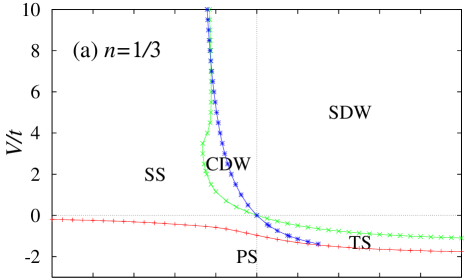
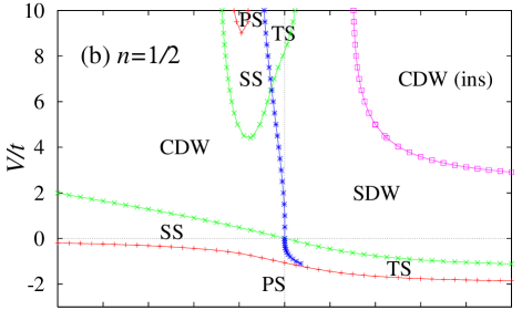
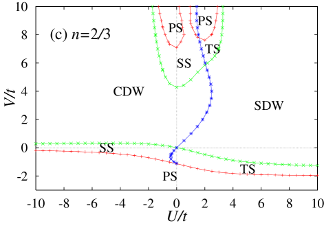
FIG. 7.: Phase diagrams of the 1D extended Hubbard model determined by the data of $L=12$ systems at (a) $n=1/3$, (b) $n=1/2$, (c) $n=2/3$ (SDW (TS): TL liquid phase with $K_{\rho}<1$ ($K_{\rho}>1$), CDW (SS): spin-gap phase with $K_{\rho}<1$ ($K_{\rho}>1$), PS: phase-separated state).

FIG. 8.: Two phase-separated states which appear in the $V/t\gg 1$ region of Fig.7(c). (a) is located in $U/t>0$ side. (b) lies in $U/t<0$ side. Spin-gap phase boundary exists between these two phase-separated states in the phase diagram.

FIG. 9.: Extrapolated value of $(x_{\sigma}^{\rm singlet}+3x_{\sigma}^{\rm triplet})/4$ and the scaling dimensions for the singlet and the triplet excitations for $L=16$ system at $n=1/2$. (a) is the case of $V/t=2$, and (b) is the case of $V/t=8$.

	basis A		basis B
	${\cal P}$	${\cal T}$	${\cal P}$	${\cal T}$	$k$	BC
Ground state	$1$	$1$	$\pm 1$	$\pm 1$	$0$	$\mp 1$
Singlet	$1$	$1$	$\pm 1$	$\pm 1$	$0$	$\pm 1$
Triplet ($S^{z}=0$)	$-1$	$-1$	$\mp 1$	$\mp 1$	$0$	$\pm 1$
Triplet ($S^{z}=1$)	$1$	$*$	$\mp 1$	$*$	$0$	$\pm 1$

TABLE I.: Discrete symmetries of wave functions for different two bases (${\cal P}$: space inversion, ${\cal T}$: spin reversal, $k$:wave number BC: boundary conditions). The upper (lower) sign denotes the case of $N/2=$even (odd). These correspondences are explained by the Perron-Frobenius theorem and the bosonization theory.

REFERENCES

- [1] E-mail address: masaaki@ginnan.issp.u-tokyo.ac.jp
- [2] E-mail address: kitazawa@stat.phys.kyushu-u.ac.jp
- [3] E-mail address: knomura@stat.phys.kyushu-u.ac.jp
- [4] A. A. Ovchinnikov, Zh. Eksp. Teor. Fiz. 57, 2137 (1969) [Sov. Phys. JETP 30, 1160 (1970)].
- [5] H. Shiba, Prog. Theor. Phys. 48, 2171 (1972).
- [6] M. Nakamura, K. Nomura, and A. Kitazawa, Phys. Rev. Lett. 79, 3214 (1997).
- [7] M. Nakamura, J. Phys. Soc. Jpn. 67, 717 (1998).
- [8] S. Tomonaga, Prog. Theor. Phys. 5, 544 (1950); J. M. Luttinger, J. Math. Phys. 4, 1154 (1963); D. C. Mattis and E. H. Lieb, J. Math. Phys. 6, 304 (1965).
- [9] F. D. M. Haldane, J. Phys. C 14, 2585 (1981).
- [10] V. J. Emery, in Highly Conducting One-Dimensional Solids, edited by J. T. Devreese et al. (Plenum, New York, 1979), p.327.
- [11] J. Sólyom, Adv. Phys. 28, 201 (1979).
- [12] J. Voit, Rep. Prog. Phys. 57, 977 (1995).
- [13] N. Manyhárd and J. Sólyom, J. Low Temp. Phys. 12, 529 (1973); J. Sólyom, ibid 547 (1973).
- [14] I. Affleck, D. Gepner, H. J. Schulz, and T. Ziman, J. Phys. A 22, 511 (1989).
- [15] T. Ziman and H. J. Schulz, Phys. Rev. Lett. 59, 140 (1987).
- [16] R. Julien and F. D. M. Haldane, Bull. Am. Phys. Soc. 28, 344 (1983); K. Okamoto and K. Nomura, Phys. Lett. A 169, 433 (1992); S. Eggert, Phys. Rev. B 54, 9612 (1996).
- [17] K. Penc and F. Mila, Phys. Rev. B 49, 9670 (1994).
- [18] K. Sano and Y. Ōno, J. Phys. Soc. Jpn. 63, 1250 (1994).
- [19] H. Q. Lin, et al., The Hubbard Model, Edited by D. Baeriswyl et al., (Plenum Press, New York, 1995) p.315.
- [20] P. -A. Bares and G. Blatter, Phys. Rev. Lett. 64, 2567 (1990); P. -A. Bares, G. Blatter, and M. Ogata, Phys. Rev. B 44, 130 (1991).
- [21] N. Kawakami and S. K. Yang, Phys. Rev. Lett. 65, 2309 (1990); J. Phys. Condens. Matter 3, 5983 (1991).
- [22] M. Ogata, M. U. Luchini, S. Sorella, and F. F. Asaad, Phys. Rev. Lett. 66, 2388 (1991).
- [23] C. S. Hellberg and E. J. Mele, Phys. Rev. B 48, 646 (1993).
- [24] Y. C. Chen and T. K. Lee, Phys. Rev. B 47, 11548 (1993).
- [25] H. Yokoyama and M. Ogata, Phys. Rev. Lett. 67, 3610 (1991); Phys. Rev. B 53, 5758 (1996).
- [26] K. Sano and K. Takano, J. Phys. Soc. Jpn. 62, 3809 (1993); K. Takano and K. Sano, Phys. Rev. B 48, 9831 (1993).
- [27] M. Ogata, M. U. Luchini and T. M. Rice, Phys. Rev. B 44, 12083 (1991).
- [28] M. Imada, J. Phys. Soc. Jpn. 60, 1877 (1991); Phys. Rev. B 48, 550 (1993).
- [29] E. Dagotto and J. Riera, Phys. Rev. B 46, 12084 (1992).
- [30] M. Troyer, H. Tsunetsugu, T. M. Rice, J. Riera, and E. Dagotto, Phys. Rev. B 48, 4002 (1993).
- [31] B. Ammon, M. Troyer, and H. Tsunetsugu, Phys. Rev. B 52, 629 (1995).
- [32] C. K. Majumder, J. Phys. C 3, 911 (1970); C. K. Majumder and D. K. Ghosh, J. Math. Phys. 10, 1399 (1969).
- [33] B. S. Shastry and B. Sutherland, Phys. Rev. Lett. 47, 964 (1981).
- [34] P. M. van den Broek, Phys. Lett. A 77, 261 (1980).
- [35] H. J. Schulz, Phys. Rev. Lett. 64, 2831 (1990); Int. J. Mod. Phys. B 5, 57 (1991).
- [36] H. W. J. Blöte, J. L. Cardy, and M. P. Nightingale, Phys. Rev. Lett. 56, 742 (1986); I. Affleck, Phys. Rev. Lett. 56, 746 (1986).
- [37] J. L. Cardy, J. Phys. A 17, L385 (1984).
- [38] F. Woynarovich, J. Phys. A 22, 4243 (1989).
- [39] In these transformation, we fix the number of electrons and of spins ( Const.). Therefore, we do not consider the variation of fields.
- [40] J. M. Kosterlitz, J. Phys. C 7, 1046 (1974).
- [41] V. Knizhnik and A. B. Zamolodchikov, Nucl. Phys. B 247, 83 (1984).
- [42] D. Gepner and E. Witten, Nucl. Phys. B 278, 493 (1986).
- [43] T. Giamarchi and H. J. Schulz, Phys. Rev. B 39, 4620 (1989).
- [44] J. L. Cardy, Nucl. Phys. B 270, 186 (1986).
- [45] P. Reinicke, J. Phys. A 20, 5325 (1987).
- [46] D. J. Amit, Y. Y. Goldschmidt, and G. Grinstein, J. Phys. A 13, 585 (1980).
- [47] C. Destri, Phys. Lett. B 210, 173 (1988); ibid 213, 565E (1988).
- [48] K. Nomura, Phys. Rev. B 48 16814, (1993).
- [49] For example, in the Lanczos algorism, energy spectra can be classified according to symmetries by choosing the initial vector.
- [50] E. Lieb, T. Schultz, and D. Mattis, Ann. Phys. 16 407 (1961); E. Lieb and D. Mattis, J. Math. Phys. 3 749 (1962).
- [51] M. Ogata and H. Shiba, Phys. Rev. B 41, 2326 (1989).
- [52] W. Kohn, Phys. Rev. 133, A171 (1964); B. S. Shastry and B. Sutherland, Phys. Rev. Lett. 65, 243 (1990).
- [53] N. Kawakami and S. K. Yang, Phys. Lett. A 148, 359 (1990).
- [54] H. Frahm and V. E. Korepin, Phys. Rev. B 42, 10553 (1990).
- [55] A system with twisted boundary conditions is transformed into a system with flux by the unitary operator . In this transformation, the wave number in the former system shifts to .
- [56] H. Q. Lin, Phys. Rev. B 44, 4676 (1991).
- [57] Y. Kuramoto and H. Yokoyama, Phys. Rev. Lett. 67, 1338 (1991).
- [58] M. Nakamura, in preparation.
- [59] J. C. Slater, H. Statz and G. F. Koster, Phys. Rev. 91, 1323 (1953).
- [60] For example, see K. Yosida, Theory of Magnetism, (Springer-Verlag, Berlin, Heidelberg 1996).