Simulation of a cusped bubble rising in a viscoelastic fluid with a new numerical method

Abstract

We developed a new lattice Boltzmann method that allows the simulation of two-phase flow of viscoelastic liquid mixtures. We used this new method to simulate a bubble rising in a viscoelastic fluid and were able to reproduce the experimentally observed cusp at the trailing end of the bubble.

I Introduction

The study of viscoelastic fluids is of great scientific interest and industrial relevance. Viscoelastic fluids are fluids that show not only a viscous flow response to an imposed stress, as do Newtonian fluids, but also an elastic response. Viscoelastic effects are almost universally observed in polymeric liquids[1], where they often dominate the flow behavior. They can also be observed in simple fluids, especially in high frequency testing[2] or in under-cooled liquids[3]. Because most research into viscoelastic liquids, especially that with an eye toward engineering applications, is directed toward polymeric liquids, the viscoelastic behavior of simple liquids is not as well known among researchers. The fact that the manifestation of viscoelasticity does not require the presence of polymer molecules is at the heart of our approach, as will become clear in the description of the viscoelastic model.

Although in most practical problems involving polymeric materials the viscosities of the materials involved are so large that the creeping flow approximation is valid, the non-linearity introduced by the viscoelastic response of the liquid makes it difficult to treat any but the most simple cases analytically. In engineering applications the situation is often further complicated by the fact that the system is comprised of several immiscible or partially miscible components with different viscoelastic properties. Examples of this include polymer blending, where two immiscible polymers are melted and mixed in an extruder, and the recovery of an oil-and-water mixture from porous bed rock. Simulation of these systems is very important, but due to the complexities only few numerical approaches exist to date. Boundary element methods have been used to simulate such systems with varying degrees of success, but the allowable complexity of the interface morphology is very limited in such approaches. Lattice Boltzmann simulations have been shown to be very successful for Newtonian two-component systems with complex interfaces[4], but for viscoelastic fluids the lattice Boltzmann models, derived by Giraud et al.[5, 6], are limited to one-component systems.

(a)

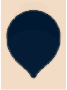
(b)

FIG. 1.: (a) An air bubble rising in $\mbox{Ivory}^{\bigcirc\!\!\!\!\!\mbox{\rm R}}$ soap and (b) the simulation results for a low viscosity drop rising in a Oldroyd B fluid on a 256x1024 lattice for a drop of radius $R_{0}=35$. The simulated bubble has a cusp that is rounded at the tip due to the finite thickness of the interface ($\sim 3$ lattice spacings).

In this article we report the successful combination of both two-component and viscoelastic features into a two-dimensional lattice Boltzmann model. We used this model to simulate a bubble rising in a viscoelastic liquid (see Figure 1) and in this letter report the first successful simulation of the experimentally observed cusp.

II Lattice Boltzmann

We use a two-dimensional lattice Boltzmann model on a square lattice with a velocity set of $\{{\bf v}_{i}\}=\{(0,0)$, $(0,1)$, $(1,0)$, $(0,-1)$, $(-1,0),$ $(1,1),$ $(-1,1)$, $(-1,-1)$, $(1,-1)\}$ and a corresponding set of densities $\{f_{i}\}$, but following Giraud et al.[6] we introduce two densities for each non-zero velocity. We use a BGK lattice Boltzmann equation that contains the full collision matrix $\Lambda_{ij}$

$$f_{i}(x+v_{i}\Delta t,t+\Delta t) = f_{i}(x,t)$$ (2)

$$+\Delta t\Lambda_{ij}(f_{j}^{0}(x,t)-f_{j}(x,t))$$

where the summation rule for repeated indices is implied and the required properties of the equilibrium distributions $f_{i}^{0}$ are discussed below. The local density is given by $\rho=\sum_{i}f_{i}$ and the momentum by $\rho{\bf u}=\sum_{i}f_{i}{\bf v}_{i}$.

In order to simulate a two-component mixture we define a second set of nine densities, $\{g_{i}\}$, with an appropriate equilibrium distribution, $\{g_{i}^{0}\}$. These densities represent the density difference of the two components A and B as $\phi=\sum g_{i}=\rho_{A}-\rho_{B}$, where the total density introduced earlier is $\rho=\rho_{A}+\rho_{B}$. For the $g_{i}$s we choose a single relaxation time lattice Boltzmann equation

$$g_{i}(x+v_{i}\Delta t,t+\Delta t) = g_{i}(x,t)$$ (4)

$$+\frac{\Delta t}{\tau}(g_{i}^{0}(x,t)-g_{i}(x,t)),$$

where $\tau$ is the relaxation time and $g_{i}^{0}$ is the equilibrium distribution.

To use the lattice Boltzmann method in order to simulate fluid flow, mass and momentum conservation have to be imposed. Mass and momentum conservation are equivalent to constraints on the equilibrium distributions:

$$\sum_{i}f_{i}^{0}=\rho,\;\;\;\sum_{i}g_{i}^{0}=\phi,\;\;\;\sum_{i}f_{i}^{0}{\bf v}_{i}=\rho{\bf u}.$$ (5)

There will be further constraints on the permissible equilibrium distributions in order for the corresponding macroscopic equations to be isotropic and to simulate the systems in which we are interested. In the next two subsections we will summarize the physics that we want to incorporate and then we will discuss how it imposes constraints on the equilibrium distributions and eigenvalues.

A Binary mixtures

To simulate a binary mixture we follow the approach of Orlandini et al. [7] and begin with a free energy functional $\Psi$ that consists of the free energy for two ideal gases and an interaction term as well as a non-local interface term:

$$\Psi[\rho_{A},\rho_{B}] = \int_{\bf x}\left[T\rho_{A}\ln(\rho_{A})+T\rho_{B}\ln(\rho_{B})\right.$$ (7)

$$\left.+\lambda\rho_{A}\rho_{B}+\kappa|\partial_{\bf x}(\rho_{A}-\rho_{B})|^{2}\right]d{\bf x},$$

where the densities $\rho_{A}$ and $\rho_{B}$ are functions of ${\bf x}$. The repulsion of the two components is introduced in the $\lambda$ term and $\kappa$ is a measure of the energetic penalty for an interface. When we write this free energy functional in terms of the total density, $\rho$, and the density difference, $\phi$, we can derive the chemical potential, $\mu$, and the pressure tensor, $P_{\alpha\beta}$, as[8]:

$$\mu = \frac{\delta\Psi}{\delta\phi}=\partial_{\phi}\Psi-\kappa\partial_{\gamma}\partial_{\gamma}\phi,$$ (8)

$$P_{\alpha\beta} = (\rho\partial_{\rho}\Psi+\phi\partial_{\phi}\Psi)\delta_{\alpha\beta}$$ (10)

$$+\kappa(\partial_{\alpha}\phi\partial_{\beta}\phi-\frac{1}{2}\partial_{\gamma}\phi\partial_{\gamma}\phi\delta_{\alpha\beta}-\phi\partial_{\gamma}\partial_{\gamma}\phi\delta_{\alpha\beta}),$$

where $\delta$ indicates a functional derivative and $\delta_{\alpha\beta}$ is the Kronecker delta. For a two-component model we fix the further moments of the equilibrium distributions[8]:

$$\sum_{i}g_{i}^{0}{\bf v}_{i} = \phi{\bf u},$$ (11)

$$\sum_{i}f_{i}^{0}v_{i\alpha}v_{i\beta} = P_{\alpha\beta}+\rho u_{\alpha}u_{\beta},$$ (12)

$$\sum_{i}g_{i}^{0}v_{i\alpha}v_{i\beta} = \mu\delta_{\alpha\beta}+\phi u_{\alpha}u_{\beta}.$$ (13)

Thus far, the model allows us to simulate a binary mixture that phase separates below a critical temperature of $T_{c}=\lambda/2$. The surface tension, $\sigma$, can be calculated analytically for a flat equilibrium interface $\phi(y)$ orthogonal to the y direction as $\sigma=\kappa\int_{-\infty}^{\infty}(\partial_{y}\phi(y))^{2}dy$ where the equilibrium density profile of $\phi$ also depends on $\kappa$.

III Viscoelasticity and the Boltzmann equation

Viscoelasticity was first proposed by Maxwell in his dynamic theory of gases[9]. He used the simple argument that in the limit where there are no intermolecular collisions the fluid in a container should behave like a solid: “…Then it can easily be shown that the pressures on the sides of the vessel due to the impacts of the molecules are perfectly independent of each other, so that the mass of moving molecules will behave, not like a fluid, but like a solid.” He goes on to deduce that the observed viscous behavior of fluids is due to binary collisions that randomize the directions of stress in the fluid. Since the collisions are fast, but not instantaneous, the elastic properties of the fluid are not completely lost, leading to the Maxwell model of viscoelasticity.

Subsequently, derivations of hydrodynamics from the dynamic theory of gases have made the approximation of a purely viscous behavior because of the difficulties of deriving a continuum approach at the length scales of a mean free path of a molecule. In gases where lengths less than the mean free path are important kinetic theory for rarefied gases is used.

There has recently been much activity in the research of the experimentally observed viscoelastic behavior of simple liquids that are undercooled. In this case, however, viscoelasticity is not obtained because the relevant length scales were of the order of a mean free path, but rather because of the correlations of subsequent collisions as described in the mode coupling theory[3].

The arguments of Maxwell, however, are still valid for describing the behavior of the Boltzmann equation, and viscoelastic properties can be derived from the Boltzmann equation if the decay of viscous stresses is slow.

The approach by Giraud et al. aims not at deriving a convected Maxwell fluid, but a convected Jeffreys fluid which is a mixture of a Maxwell fluid with a Newtonian fluid. A double set of densities is introduced allowing two stresses, one of which is chosen to relax quickly and is, therefore, a viscous stress, and the other, which is chosen to decay very slowly, represents a viscoelastic stress. The resulting model is a convected Jeffreys model that is often used to describe a polymeric fluid in a solvent. Care has to be taken for the choice of the collision matrix and the equilibrium distribution to ensure an isotropic model. The details of this one-component model are described in the publication by Giraud et al.[6]

A Chapman-Enskog expansion of the lattice Boltzmann equations (2) and (4) gives the macroscopic equations that our system simulates. Mass conservation gives the continuity equation:

$$\partial_{t}\rho+\partial_{\alpha}(\rho u_{\alpha})=0.$$ (14)

Momentum conservation gives a Navier Stokes equation:

$$\rho\partial_{t}u_{\alpha}+\rho u_{\beta}\partial_{\beta}u_{\alpha}=-\partial_{\beta}\left(P_{\alpha\beta}+\sigma^{v}_{\alpha\beta}+\sigma_{\alpha\beta}\right)$$ (15)

where the viscous stress is given by

$$\sigma^{v}_{\alpha\beta}=\nu_{\infty}\partial_{\beta}(\rho u_{\alpha})+\xi_{\infty}\partial_{\gamma}(\rho u_{\gamma})\delta_{\alpha\beta}.$$ (16)

The viscoelastic stress has the constitutive relation

$$\sigma_{\alpha\beta}+\theta\sigma_{(1)\alpha\beta}=-(\nu_{0}-\nu_{\infty})\left(\partial_{\alpha}(\rho u_{\beta})+\partial_{\beta}(\rho u_{\alpha})\right)$$ (17)

where $\sigma_{(1)}$ represents the upper convected derivative of $\sigma$. These equations are equivalent to the Navier-Stokes and Jeffreys equations only in the incompressible limit where $\partial_{\alpha}(\rho u_{\beta})=\rho\partial_{\alpha}u_{\beta}$. The fully compressible equations can only be simulated when a larger set of velocities is used[10]. The conservation of the density difference leads to the convection diffusion equation

$$\partial_{t}\phi+\partial_{\alpha}(\phi u_{\alpha})=D\partial_{\alpha}\partial_{\alpha}\mu+\partial_{\beta}\left(\frac{\phi}{\rho}\partial_{\alpha}(P_{\alpha\beta}-\sigma_{\alpha\beta})\right)$$ (18)

where $D$ is a diffusion constant given by $D=(\tau-1/2)$.

IV Simulation of a bubble in a viscoelastic liquid

We applied our method to a system similar to the experimentally well-studied system of an air bubble rising in a viscoelastic fluid. In our simulation we represent the bubble using a phase-separated Newtonian drop of low viscosity in matrix which is viscoelastic by letting the relaxation time $\theta$ in equation (17) depend smoothly on the density difference $\phi$ between $\theta=0.05$ in the drop and $\theta=66$ in the surrounding fluid. We choose $\xi_{\infty}=0.06$, $\nu_{\infty}=0.01$, and $\nu_{0}=0.01$ in the drop and $\nu_{0}=0.175$ outside. For the thermodynamic parameters we select $T=0.5$, $\lambda=1.1$, and $\kappa=0.007$, which corresponds to a surface tension of $\sigma=0.02$. All units are in terms of the lattice spacings and the time steps $\Delta t=\Delta x=1$. We introduce a forcing dependent on $\phi$ so that the bubble is forced upward while the surrounding fluid is forced downward. We choose the total change in the momentum due to the forcing to be zero so that no walls are required in the simulations.

We start the simulations without forcing and then periodically increase the forcing after $10,000$ to $40,000$ iterations. We observe the change in the velocity $u$ and store the distribution of $\phi$ so that we have a way of judging the deformation of the bubble.

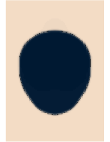
(a)

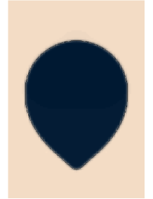
(b)

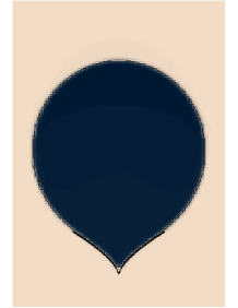
(c)

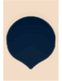
(d)

FIG. 2.: Shape for the simulated bubbles for different forcings in (lattice spacings)/$\mbox{(time step)}^{2}$: (a) $1.6\cdot 10^{-5}$, (b) $3.6\cdot 10^{-5}$, (c) $9.6\cdot 10^{-5}$, and (d) $1.96\cdot 10^{-4}$. In (c) a fit to the predicted form of the cusp ($|x|^{2/3}$ is also shown. All simulations are after a 20,000 iterations at this forcing.

Figure 2 shows the form of the drop for different forcings. At low forcings the drop is elongated in the flow direction. This is in direct contrast to a bubble in a Newtonian fluid, which is flattened in the flow direction. At a larger forcing the bubble forms a cusp at the lower tip of the drop. For even larger forcings the drop starts to flatten in the flow direction. This sequence is in agreement with the experimental findings[11]. The elongation of a rising bubble has been simulated before[12], but this is the first time that the formation of a cusp has been simulated. In Figure 2(c) it is shown that the cusp can be fitted to the functional form $|x|{2/3}$ predicted by Joseph et al.[13] for a two-dimensional cusp created by the flow induced by two couter-rotating cylinders.

Experimentally the formation of a cusp has been observed to coincide with a jump of nearly an order of magnitude in the terminal velocity of the bubble[1, 11], although the mechanism remains disputed. On the one hand Bird et al. argue that surface-active impurities tend to immobilize bubble surfaces and hence retard the motion of gas bubbles. This discontinuous change in bubble shape may be responsible for the removal of the impurities, and thus lead to a jump in the final velocity. Liu[11] et al. alternatively suggest that the change in the shape of the bubble will make it more streamlined, and therefore increase the terminal velocity.

FIG. 3.: Velocity, u, of the bubble in two different sets of simulations for a bubble of radius 35 in a 256x512 lattice. On the x-axis the iterations were multiplied by a scale factor so that corresponding forcings appear at the same point in the graph. No jump in the final velocity is observed at $\sim 0.5\;10^{6}$ iterations where the formation of a cusp is observed (indicated by arrow). The scale factors were 0.25 and 1. Velocity is measured in lattice units per time step.

We examined the velocity for the rising drop as described above and found no jump of about half an order of magnitude as observed by Liu et al. in their experiment (see Figure 1). Our simulations suggest that the jump in velocity they observe is not connected to a more streamline form of the bubble due to the cusp, but more likely to the presence of surfactants that are absent in our simulations.

V Conclusion

We introduced a lattice Boltzmann model that can simulate viscoelastic two-component flows. We gave an intuitive explanation of the origin of viscoelasticity in our model and the model by Giraud et al. in terms of the original theory of Maxwell[9]. Simulations using this method have succeeded in reproducing the cusp at the end of a bubble rising in a viscoelastic medium that have eluded earlier numerical attempts with a more traditional boundary integral approach.

The model has been successful in the qualitative simulation of the bubble problem in two dimensions. We intend to extend the model to three dimensions in the future. This will also enable us to compare the results quantitatively with experiment.

REFERENCES

- [1] R.B. Bird, R.C. Armstrong, O. Hassager, Dynamics of Polymeric Liquids, second edition (1987), John Wiley & sons, New York.
- [2] J.P. Boon and S. Yip, Molecular hydrodynamics, first edition (1980), McGraw-Hill.
- [3] W. Götze and L. Sjögren, Transp. Th. and Stat. Phys. 24, 801 (1995).
- [4] A.J. Wagner and J.M. Yeomans, Phys. Rev. Lett. 80, 1429 (1998).
- [5] L. Giraud, D. d’Humières, and P. Lallemand, Euro. Phys. Lett. 42, 625 (1998).
- [6] L. Giraud and D. d’Humières, Non-linear viscoelastic models using the Lattice Boltzmann Method, in preparation.
- [7] E. Orlandini, M.R. Swift and J.M. Yeomans, Euro. Phys. Lett. 32, 463 (1995).
- [8] A.J. Wagner and J.M. Yeomans, Phase separation under shear in two-dimensional binary fluids, accepted for publication in Phys. Rev. E.
- [9] J.C. Maxwell, Phil. Trans. Roy. soc. A157, 49 (1867).
- [10] A. J. Wagner, D. Phil. thesis, Oxford University , (1998).
- [11] Y.J. Liu, T.Y. Liao and D.D. Joseph, J. Fluid Mech. 304, 321 (1995).
- [12] D.S. Noh, I.S. Kang and L.G. Leal, Phys. Fluids A 5, 1315 (1993).
- [13] D.D. Joseph, J. Nelson, M. Renardy and Y. Renardy, J. Fluid Mech. 223, 383 (1991).
-
[14]
More information on the parallel programming language ZPL can be found
at:
http://www.cs.washington.edu/research/zpl/