*

Abstract

We briefly introduce hysteresis in spatially extended systems and the dynamic phase transition observed as the frequency of the oscillating field increases beyond a critical value. Hysteresis and the decay of metastable phases are closely related phenomena, and a dynamic phase transition can occur only for field amplitudes, temperatures, and system sizes at which the metastable phase decays through nucleation and growth of many droplets. We present preliminary results from extensive Monte Carlo simulations of a two-dimensional kinetic Ising model in a square-wave oscillating field and estimate critical exponents by finite-size scaling techniques adapted from equilibrium critical phenomena. The estimates are consistent with the universality class of the two-dimensional equilibrium Ising model and inconsistent with two-dimensional random percolation. However, we are not aware of any theoretical arguments indicating why this should be so. Thus, the question of the universality class of this nonequilibrium critical phenomenon remains open.

1 Introduction

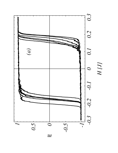
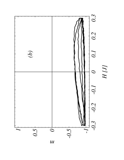
Figure 1: Series of hysteresis loops obtained from a Monte Carlo (MC) simulation of a two-dimensional kinetic Ising ferromagnet at $T\!=\!0.8\ T_{\mathrm{c}}$ in a sinusoidally varying field. The dimensionless magnetization $m$ is shown vs. the field $H$ in units of the nearest-neighbor interaction energy $J$. (a): A series of regular symmetric hysteresis loops, typical of a system driven at a moderately low frequency. (b): A series of asymmetric hysteresis loops, typical of a system driven at a high frequency

Hysteresis often occurs when a bistable or multistable system is driven by an oscillating force which varies too fast for the system to respond without a phase lag. In fact, the word was coined by Ewing from the Greek husterein ($\stackrel{{\scriptstyle\scriptscriptstyle c}}{{\upsilon}}\!\!\sigma\tau\epsilon\rho\acute{\epsilon}\omega$) which means “to be behind” [1]. Examples include ferromagnets and ferroelectrics in AC fields, electrochemical cyclic-voltammetry experiments, and nonlinear elastic media under oscillating stress, just to mention a few. The most familiar representation of hysteresis is probably the (usually) closed curve obtained by plotting the system response versus the applied force. Examples of such hysteresis loops are shown in Fig. 1(a). This figure shows data from a Monte Carlo (MC) simulation of a two-dimensional kinetic Ising ferromagnet below its critical temperature, which is driven by a sinusoidally oscillating field. However, the shape of the loops shown is quite general. For simplicity and concreteness, in this paper we use magnetic language, designating the oscillating force the “field” and the system response the “magnetization”. These quantities can easily be re-interpreted when one discusses other types of systems, such as those mentioned above.

Hysteresis was first systematically investigated in the late 19th century by engineers and physicists primarily concerned with the development of electric motors and transformers [1, 2, 3, 4, 5]. The area of the hysteresis loop is proportional to the magnetic energy loss during one field period, as was first pointed out by Warburg [2]. Its dependences on the frequency and amplitude of the applied field have therefore been studied intensively ever since, but open questions still remain. In particular, the question of whether the low-frequency behavior for ultrathin films of highly anisotropic materials is asymptotically a power law or logarithmic is still under investigation, both experimentally [6, 7, 8, 9, 10] and theoretically [11, 12, 13, 14, 15, 16, 17].

A different aspect of hysteresis in bistable systems, which is the main topic of the present paper, occurs at higher driving frequencies. When the frequency becomes sufficiently high, the symmetry of the hysteresis loop, which is apparent in Fig. 1(a), is broken. Instead of oscillating between its two stable values with a phase lag relative to the field, the magnetization oscillates around one or the other of its zero-field stable values. A series of such asymmetric loops is shown in Fig. 1(b). This symmetry breaking has become a topic of vigorous research during the last two decades. It was first reported by Tomé and de Oliveira [18], who observed it during numerical solutions of a mean-field equation of motion for a ferromagnet in an oscillating field.

Subsequently, symmetry breaking has been observed in numerous MC simulations of kinetic Ising systems, [17, 19, 20, 21, 22, 23, 24], as well as in further mean-field studies [20, 22, 23, 25]. It may also have been experimentally observed in ultrathin films of Co on Cu(001) [7, 8]. Reviews of the field as it stood in 1994 and as it stands today can be found in [26] and [27], respectively. There now appears to be a consensus that the symmetry breaking corresponds to a genuine second-order, nonequilibrium phase transition. Associated with the transition is a divergent time scale (critical slowing-down [22] and, for spatially extended systems, a divergent correlation length [17, 24]. Although estimates of the critical exponents have recently become available from finite-size scaling analyses of MC data for a two-dimensional Ising system in a sinusoidally oscillating field [17, 24], their accuracy is not yet sufficient to decide whether the dynamic phase transition in this system belongs to a previously known universality class or represents a new one. Neither are we aware of theoretical arguments that can resolve the issue or help to identify the correct “critical clusters”.

The main purpose of this paper is to present preliminary results for two-dimensional kinetic Ising systems in square-wave oscillating fields. These may help point the way towards answering some of the remaining questions concerning this intriguing nonequilibrium critical phenomenon. The use of a square-wave field both tests the universality of the dynamic phase transition and significantly increases the computational speed. The structure of the remainder of the paper is as follows. The kinetic model system and the relevant quantities, including the dynamic order parameter, are defined in Sect. 2. A brief primer on metastable decay in spatially extended systems is given in Sect. 3. Numerical results are presented in Sect. 4, and a discussion and some suggestions for further research are given in Sect. 1.

2 Model and Relevant Quantities

Most numerical simulations of the dynamic phase transition (hereafter abbreviated DPT) in spatially extended systems have been performed on nearest-neighbor kinetic Ising ferromagnets on hypercubic lattices with periodic boundary conditions. These models are defined by the Hamiltonian

$${\cal H}=-J\sum_{{\langle ij\rangle}}{s_{i}s_{j}}-H(t)\sum_{i}{s_{i}}\;,$$ (1)

where $s_{i}\!=\!\pm 1$ is the state of the $i$th spin, $\sum_{{\langle ij\rangle}}$ runs over all nearest-neighbor pairs, $J>0$ is the ferromagnetic interaction, $\sum_{i}$ runs over all $L^{d}$ lattice sites, and $H(t)$ is an oscillating, spatially uniform applied field. The magnetization per site is

$${m(t)}={L^{-d}}\sum_{i=1}^{L^{d}}{s_{i}(t)}\;.$$ (2)

The temperature $T$ is fixed below its zero-field critical value $T_{\mathrm{c}}$, so that the magnetization for $H\!=\!0$ has two degenerate spontaneous equilibrium values, $\pm m_{\mathrm{sp}}(T)$. For nonzero fields the equilibrium magnetization has the same sign as $H$, while for not too strong $H$ (see Sect. 3 for quantitative statements) the opposite magnetization direction becomes metastable and decays slowly towards equilibrium with time.

The dynamic used here, as well as in [17] and [24], is the Glauber single-spin-flip MC algorithm with updates at randomly chosen sites [28]. The time unit is one MC step per spin (MCSS). Each attempted spin flip from ${s_{i}}$ to ${-s_{i}}$ is accepted with probability

$$W(s_{i}\rightarrow-s_{i})=\frac{\exp(-\beta\Delta E_{i})}{1+\exp(-\beta\Delta E_{i})}\;.$$ (3)

Here $\Delta E_{i}$ is the energy change that would result from accepting the spin flip, and $\beta\!=\!1/k_{\rm B}T$ where $k_{\rm B}$ is Boltzmann’s constant. For the largest system ($L\!=\!512$ square lattice) we employed a massively parallel implementation of this algorithm [29, 30, 31, 32]. Other dynamics that have been used in MC studies of the DPT are Glauber or Metropolis [28] with updates at sequentially selected sites [20, 21, 22, 23, 26, 27]. Although the choice of update scheme can lead to subtle differences in the dynamics [33] and we prefer random site selection as the more physical scheme, we do not believe it affects universal aspects of the DPT.

The dynamic order parameter is the period-averaged magnetization [18],

$$Q=\frac{1}{2t_{1/2}}\oint m(t)\ {\mathrm{d}}t\;,$$ (4)

where $t_{1/2}$ is the half-period of the oscillating field, and the beginning of the period is chosen at a time when $H(t)$ changes sign. Analogously we also define the local order parameter

$$Q_{i}=\frac{1}{2t_{1/2}}\oint s_{i}(t)\ {\mathrm{d}}t\;,$$ (5)

which is the period-averaged spin at site $i$. For slowly varying fields the probability distribution of $Q$ is sharply peaked at zero [17]. We shall refer to this as the dynamically disordered phase. For rapidly oscillating fields the $Q$ distribution becomes bimodal with two sharp peaks near $\pm m_{\mathrm{sp}}(T)$, corresponding to the broken symmetry of the hysteresis loops [17]. We shall refer to this as the dynamically ordered phase. Near the DPT we use finite-size scaling analysis of MC data to estimate the critical exponents that characterize the transition.

Previous studies of the DPT have used an applied field which varies sinusoidally in time. While sinusoidal or linear saw-tooth fields are the most common in experiments and are necessary to obtain a vanishing loop area in the low-frequency limit [16, 17], the wave form of the field should not affect universal aspects of the DPT. This should be so because the transition essentially depends on the competition between two time scales: the half-period $t_{1/2}$ of the applied field, and the average time it takes the system to leave the metastable region near one of its two degenerate zero-field equilibria when a field of magnitude $H_{0}$ and sign opposite to the magnetization is applied. This metastable lifetime, $\langle\tau(H_{0},T)\rangle$, is usually estimated as the average first-passage time to zero magnetization. In the present paper we use a square-wave field of amplitude $H_{0}$. This has significant computational advantages over the sinusoidal field variation since we can use two look-up tables to determine the acceptance probabilities: one for $H\!=\!+H_{0}$ and one for $H\!=\!-H_{0}$.

In terms of the dimensionless half-period,

$$\Theta=t_{1/2}\left/\langle\tau(H_{0},T)\rangle\right.\;,$$ (6)

the DPT should occur at a critical value $\Theta_{\mathrm{c}}$ of order unity. Although $\Theta$ can be changed by varying either $t_{1/2}$, $H_{0}$, or $T$, in a first approximation we expect $\Theta_{\mathrm{c}}$ to be independent of $H_{0}$ and $T$. This expectation is confirmed by simulations carried out at several $H_{0}$ and $T$ for different system sizes. In particular, Fig. 2(a) shows the average norm of the order parameter $\langle|Q|\rangle$ vs. $\Theta$ for various field amplitudes and the corresponding metastable lifetimes. For weaker fields (longer lifetimes) the transition is apparent at some $\Theta_{\mathrm{c}}\sim 1$, while it clearly disappears (no dynamically ordered phase exists) for sufficiently strong fields (small lifetimes). Figure 2(b) shows $\Theta_{\mathrm{c}}$ vs. $\langle\tau(H_{0},T)\rangle$ where $\Theta_{\mathrm{c}}$ was determined approximately as the location of the peak in the fluctuations of $Q$ in a $L\!=\!64$ system. Note that $\Theta_{\mathrm{c}}$ for an infinite system is slightly different from this estimate due to finite-size effects. Also, these effects are expected to be smaller for strong fields (small lifetimes) where the spins become uncorrelated. The deviations from unity for very small $\langle\tau(H_{0},T)\rangle$ and the complete disappearance of the DPT are discussed further in Sect. 3.

In many studies of the DPT the transition has been approached by changing $H_{0}$ or $T$ [19, 20, 21, 23]. While the above discussion indicates that this is correct in principle, we show in Sect. 3 that $\langle\tau(H_{0},T)\rangle$ depends strongly and nonlinearly on its arguments. We therefore prefer changing $t_{1/2}$ at constant $H_{0}$ and $T$ [17, 24], as this in practice gives more precise control over the distance from the transition.

3 Decay of Metastable Phases

In mean-field studies of the DPT $H_{0}$ must be larger than the temperature-dependent spinodal field beyond which the metastable free-energy minimum disappears [11]. For weaker fields the hysteresis loops remain asymmetric, even for the lowest frequencies. It is much less appreciated that bounds on the fields and temperatures for which a DPT can occur also exist for spatially extended systems. These bounds are readily obtained from classical nucleation theory [34] and the Kolmogorov-Johnson-Mehl-Avrami (KJMA) theory of metastable decay [17, 24, 33, 35, 36, 37] by comparing four characteristic lengths. These are the lattice constant (here defined as unity), the size $R_{\rm c}(|H|,T)$ of a randomly nucleated critical droplet of stable phase, the typical distance $R_{0}(|H|,T)$ between individual droplets, and the system size $L$.

The critical radius is determined by the competition between the surface free energy of the droplet, $\propto\sigma(T)R^{d-1}$ where $\sigma(T)$ is the surface tension between the two phases, and the bulk free energy, $\propto-|H|R^{d}$. As a result, $R_{\rm c}\propto\sigma(T)/|H|$. The nucleation rate per unit volume is $I(H,T)\propto\exp\left[-\Xi(T)/|H|^{d-1}\right]$, where $\Xi(T)$ is the field-independent part of the free energy of a critical droplet divided by $k_{\rm B}T$, and preexponential powers of $|H|$ have been suppressed.

The classical KJMA theory describes the metastable decay as homogeneous nucleation of droplets at random times and positions with nucleation rate $I$, followed by deterministic growth of these droplets with constant radial velocity $v\propto|H|$. Assuming that the droplets overlap freely when they meet, the time dependent magnetization is given by the well-known “Avrami’s Law”,

$$m(t) \approx m_{\rm sp}\left\{2\exp\left[-\int_{0}^{t}I\Omega_{d}(vt^{\prime})^{d}{\rm d}t^{\prime}\right]-1\right\}$$ (7)

$$= m_{\rm sp}\left\{2\exp\left[-\frac{\Omega_{d}v^{d}I}{d+1}t^{d+1}\right]-1\right\}\;,$$ (8)

where $\Omega_{d}$ is a proportionality constant such that the volume of a droplet of radius $R$ equals $\Omega_{d}R^{d}$. The argument of the exponential is the “extended volume” [36], i.e., the total volume fraction of stable-phase droplets, uncorrected for overlaps. Solving (8) for the time at which $m\!=\!0$ gives the lifetime,

$$\langle\tau(|H|,T)\rangle=\left[\frac{\Omega_{d}v^{d}I}{(d+1)\ln 2}\right]^{-{1}/({d+1})},$$ (9)

which depends on $|H|$ and $T$ through $v$ and $I$, but is independent of $L$. The characteristic length $R_{0}$ is obtained from $v(|H|,T)$ and $\langle\tau(|H|,T)\rangle$ as

$$R_{0}(|H|,T)=v(|H|,T)\ \langle\tau(|H|,T)\rangle\propto\exp\left[\frac{\Xi(T)}{(d+1)|H|^{d+1}}\right]\;,$$ (10)

where a preexponential power of $|H|$ again has been suppressed [33, 35].

The regime in which a DPT can occur is that in which a large number of droplets contribute to the decay of the metastable phase:

$$1\ll R_{\rm c}\ll R_{0}\ll L\;.$$ (11)

This is known as the multidroplet (MD) regime [33, 35]. It is limited on the weak-field/small-system side by the dynamic spinodal (DSP) field ,

$$H_{\rm DSP}(T,L)\sim\left(\frac{1}{d+1}\frac{\Xi(T)}{\ln L}\right)^{{1}/({d-1})}\;,$$ (12)

which corresponds to $R_{0}\!\approx\!L$. For $|H|<H_{\rm DSP}$ almost always only a single droplet contributes to the magnetization switching. A DPT does not occur in this regime, but stochastic resonance is observed at low frequencies [38]. On the strong-field side the MD regime is limited by an $L$-independent cross-over field approximately given by $2R_{\rm c}\!\approx\!1$. By a somewhat confusing term this crossover is often referred to as the “mean-field spinodal” $H_{\rm MFSP}(T)$ [33, 35]. In the strong-field (SF) regime beyond this limit the spins become increasingly uncorrelated as $|H|$ increases. This is the region of small $\langle\tau(H_{0},T)\rangle$ (large $H_{0}$) where $\Theta_{\rm c}$ rapidly approaches zero and the transition disappears (Fig. 2). In computational studies of the DPT it is essential to ensure that $H_{\rm DSP}(T,L)<H_{0}<H_{\rm MFSP}(T)$ for all values of $L$ and $T$ used.

4 Results

We performed extensive simulations on square lattices with $L$ between 64 and 512 at $T\!=\!0.8T_{\rm c}$ and $H_{0}\!=\!0.3J$. Typical run lengths near the transition range from $2$$\times$$10^{4}$ to $10^{5}$ full periods, corresponding to $2.8$$\times$$10^{6}-1.4$$\times$$10^{7}$ MCSS. The system was initialized with all spins up and and the square-wave external field started with the half-period in which $H\!=\!-H_{0}$. After some relaxation the system magnetization reaches a limit cycle (except for thermal fluctuations), i.e., $Q$ is stationary. We discarded the first 500 periods of the time series to exclude transients from the stationary-state averages.

For small half-periods ($\Theta\ll\Theta_{\rm c}$) the magnetization does not have time to switch, resulting in $|Q|\!\approx\!m_{\rm sp}$, while for large half-periods ($\Theta\gg\Theta_{\rm c}$) it switches every half-period and $Q\!\approx\!0$ as can be seen from the time series in Fig. 3. The transition between the high- and low-frequency regimes is singular, characterized by large fluctuations in $Q$. To illustrate the spatial aspects of the transition we also show configurations of the local order parameter $Q_{i}$ in Fig. 4. Below $\Theta_{\rm c}$ [Fig. 4(a)] the majority of spins spend most of their time in the $+1$ state, i.e., in the metastable phase during the first half-period, and in the stable equilibrium phase during the second half-period (except for equilibrium fluctuations). Thus, most of the $Q_{i}\!\approx\!+1$. Droplets of $s_{i}\!=\!-1$ that nucleate during the negative half-period and then decay back to $+1$ during the positive half-period show up as roughly circular gray spots in the figure. Since the spins near the center of such a droplet become negative first and revert to positive last, these spots appear darkest in the middle. Above $\Theta_{\rm c}$ [Figs. 4(c,d)] the system follows the field in every half-period (with some phase lag) and $Q_{i}\!\approx\!0$ at all sites $i$. Near $\Theta_{\rm c}$ [Fig. 4(b)] there are large clusters of both $Q_{i}\!\approx\!+1$ and $Q_{i}\!\approx\!-1$ separated by wide “interfaces” where $Q_{i}\!\approx\!0$. Also, for not too large lattices one often observes the full reversal of an ordered configuration $\{Q_{i}\}\rightarrow-\{Q_{i}\}$, typical of finite, spatially extended systems undergoing symmetry breaking.

For finite systems in the dynamically ordered phase the distribution of $Q$ becomes bimodal. Thus, to capture symmetry breaking, one has to measure the average norm of Q as the order parameter, i.e., $\langle|Q|\rangle$. Figure 5(a) clearly shows that this order parameter is of order unity for $\Theta<\Theta_{\rm c}$ and vanishes for $\Theta>\Theta_{\rm c}$, except for finite-size effects.

To characterize and quantify this transition in terms of critical exponents we employ the well-known technique of finite-size scaling [28, 39]. The quantity analogous to the susceptibility is the scaled variance of the dynamic order parameter,

$$X_{L}=L^{2}\left(\langle Q^{2}\rangle_{L}-\langle|Q|\rangle_{L}^{2}\right)\;.$$ (13)

For finite systems $X_{L}$ has a characteristic peak near $\Theta_{\rm c}$ [see Fig. 5(b)] which increases in height with increasing $L$, while no finite-size effects can be observed for $\Theta\ll\Theta_{\rm c}$ and $\Theta\gg\Theta_{\rm c}$. This implies the existence of a divergent length scale, possibly the correlation length which governs the long-distance behavior of the local order-parameter correlations $\langle Q_{i}Q_{j}\rangle$. Note that the location of the maximum in $X_{L}$ shifts with $L$. This also contains important information about the critical exponents.

To estimate the value of $\Theta_{\rm c}$ at which the transition occurs in an infinite system we use the intersection of the fourth-order cumulant ratios [28, 39],

$$U_{L}=1-\frac{\langle Q^{4}\rangle_{L}}{3\langle Q^{2}\rangle_{L}^{2}}\;,$$ (14)

for several system sizes as shown in Fig. 5(c). For the largest system ($L\!=\!512$) the error bars on $U_{L}$ were too large to use it to obtain estimates for the crossing. Our estimate for the dimensionless critical half-period is $\Theta_{\rm c}\!=\!0.913\pm 0.003$ with a fixed-point value $U^{*}\!=\!0.615\pm 0.005$ for the cumulant ratio.

For our model the quantity analogous to the reduced temperature in equilibrium systems (i.e., the distance from the critical point) is

$$\theta=\frac{|\Theta-\Theta_{\rm c}|}{\Theta_{\rm c}}\;.$$ (15)

Finite-size scaling theory provides simple relations for the order parameter and its scaled variance $X_{L}$ for finite systems in the critical regime [28, 39]:

$$\halign to=433.62pt{\@eqnsel\hskip\@centering$\displaystyle{#}$&\global\@eqcnt\@ne\hskip 2\arraycolsep\hfil${#}$\hfil&\global\@eqcnt\tw@\hskip 2\arraycolsep$\displaystyle{#}$\hfil&\llap{#}\cr 0.0pt plus 1000.0pt$\displaystyle{\langle|Q|\rangle_{L} &10.0pt\hfil${= &10.0pt$\displaystyle{L^{-\beta/\nu} {\cal F}_{\pm}(\theta L^{1/\nu}) \;, {}&\hbox to0.0pt{\hss{\rm(0.0a)}\cr\penalty 100\vskip 3.0pt\vskip 0.0pt\cr 0.0pt plus 1000.0pt$\displaystyle{X_{L} &10.0pt\hfil${= &10.0pt$\displaystyle{L^{\gamma/\nu} {\cal G}_{\pm}(\theta L^{1/\nu})\;, &\hbox to0.0pt{\hss{\rm(0.0b)}\cr}}}}}}}}}$$

where ${\cal F}_{\pm}$ and ${\cal G}_{\pm}$ are scaling functions and the $+$ ($-$) index refers to $\Theta>\Theta_{\rm c}$ ($\Theta<\Theta_{\rm c}$). Then at $\Theta_{\rm c}$ ($\theta\!=\!0$) we have the finite-size behavior of the above two observables:

$$\halign to=433.62pt{\@eqnsel\hskip\@centering$\displaystyle{#}$&\global\@eqcnt\@ne\hskip 2\arraycolsep\hfil${#}$\hfil&\global\@eqcnt\tw@\hskip 2\arraycolsep$\displaystyle{#}$\hfil&\llap{#}\cr 0.0pt plus 1000.0pt$\displaystyle{\langle|Q|\rangle_{L} &10.0pt\hfil${\propto&10.0pt$\displaystyle{L^{-\beta/\nu} \;, {}&\hbox to0.0pt{\hss{\rm(0.1a)}\cr\penalty 100\vskip 3.0pt\vskip 0.0pt\cr 0.0pt plus 1000.0pt$\displaystyle{X_{L} &10.0pt\hfil${\propto&10.0pt$\displaystyle{L^{\gamma/\nu} \;. &\hbox to0.0pt{\hss{\rm(0.1b)}\cr}}}}}}}}}$$

Using $\langle|Q|\rangle_{L}$ and $X_{L}$ for several system sizes at $\Theta_{\rm c}$ (estimated as the value of $\Theta$ where the cumulants cross) we employ (4) and (4) to find the exponent ratios $\beta/\nu$ and $\gamma/\nu$ through weighted linear least-squares fitting to the logarithmic data. Further, the shift in the location of the peak in $X_{L}$ for these finite systems, $\Theta_{\rm c}(L)$, is used to estimate $\nu$ in the same way [28, 39]:

$$|\Theta_{\rm c}(L)-\Theta_{\rm c}|\propto L^{-1/\nu}\;.$$ (2)

Our estimates for these exponents are $\beta/\nu$$=$$0.122\pm 0.005$, $\gamma/\nu$$=$$1.77\pm 0.05$, and $\nu$$=$$1.0\pm 0.15$. The largest uncertainty occurs in $\nu$ due to the large relative errors in $|\Theta_{\rm c}(L)-\Theta_{\rm c}|$. We note that these numbers are very close (within the one-standard-deviation error bars) to the critical exponents of the two-dimensional Ising universality class $\beta/\nu$$=$$1/8$$=$$0.125$, $\gamma/\nu$$=$$7/4$$=$$1.75$, and $\nu$$=$$1$. However, as discussed in Sect. 1, we do not consider this conclusive proof of the universality class for this nonequilibrium phase transition.

To obtain a more general picture of how well the scaling relations in (4) and (4) are obeyed, we plot $\langle|Q|\rangle_{L}L^{\beta/\nu}$ [Fig. 6(a)] and $X_{L}L^{-\gamma/\nu}$ [Fig. 6(b)] vs. $\theta L^{1/\nu}$ [40]. In these figures we used the exponents of the two-dimensional Ising universality class since they are within one standard deviation of our estimates and analogous data-collapse plots using our numerical exponent estimates do not look perceptibly different. The plots show excellent agreement with the scaling assumption and graphically define the scaling functions ${\cal F}_{\pm}$ and ${\cal G}_{\pm}$. The asymptotic behaviors of these functions have to be simple power laws so that the true critical behavior is restored when the limit $L\rightarrow\infty$ is taken in (4) and (4). Some deviation can be observed in Fig. 6(b): below $\Theta_{\rm c}$ the data points for the smaller systems systematically start to peel off earlier from the straight line representing the asymptotic behavior of ${\cal G}_{-}$ for large argument.

In the absence of theoretical arguments why this DPT should belong to the Ising universality class we also tested the data collapse with the exponents for random percolation, which are relatively close to the corresponding Ising ones [41]: $\beta/\nu$$=$$5/48$$\approx$$0.104$, $\gamma/\nu$$=$$43/24$$\approx$$1.79$, and $\nu$$=$$4/3$$\approx$$1.33$. It appears reasonable to consider this universality class in particular, since the metastable decay process described in Sect. 3 produces transient spanning clusters that belong to the random-percolation class as $m(t)$ passes through $H$- and $T$-dependent percolation thresholds for the two phases near $m\!=\!0$ [42]. Data-collapse plots using the random-percolation exponents are shown in Figs. 6(c,d). They are clearly inferior to the ones with the Ising exponents [Figs. 6(a,b)]. In particular, for $\Theta>\Theta_{c}$ (the dynamically disordered phase) the data collapse gets progressively worse for larger systems. Comparing the scaling plots in Figs. 6(a,b) with Figs. 6(c,d) we conclude that the exponent $\nu$ for the DPT is significantly different from that of the random percolation universality class and that it is closer to the Ising value. This conclusion is supported by direct comparison of the random-percolation and Ising exponents with our numerical estimates for the DPT. Our estimates for $\beta/\nu$ and $\nu$ lie more than two standard deviations away from the percolation values, but less than one standard deviation away from the Ising values, while our estimate for $\gamma/\nu$ lies midway between and less than one standard deviation away from the exact values for both classes.

The exponents previously obtained with a sinusoidally oscillating field [17, 38] lie within two standard deviations of our values. As it was difficult to determine the uncertainties in the estimates obtained in that study, we believe the results are consistent and indicate that the DPT in systems driven by sinusoidal and square-wave fields belong to the same universality class, as expected.

1 Summary and Discussion

In this paper we have presented preliminary results from a large-scale Monte Carlo study of the dynamic phase transition (DPT) in a two-dimensional kinetic Ising ferromagnet driven by a square-wave oscillating field. Our results are consistent with those of previous studies of the same model in a sinusoidally varying field [17, 24]. They indicate that for field amplitudes $H_{0}$ such that the metastable magnetized phase decays to equilibrium via the multidroplet (MD) mechanism described in Sect. 3, the system undergoes a continuous DPT when the half-period of the field, $t_{1/2}$, approximately equals the metastable lifetime, $\langle\tau(H_{0},T)\rangle$. Thus the critical value $\Theta_{\rm c}$ of the dimensionless half-period defined in (6) is near unity. As $\Theta$ is increased past $\Theta_{\rm c}$ the order parameter $\langle|Q|\rangle$, which is the expectation value of the norm of the period-averaged magnetization, vanishes in a singular fashion, as shown in Fig. 5(a).

The strong and systematic finite-size effects in the order parameter and its scaled variance indicate that there is a divergent correlation length associated with the transition. Using standard finite-size scaling techniques borrowed from the theory of equilibrium phase transitions we therefore estimated $\Theta_{\rm c}$ and the critical exponents $\beta$, $\gamma$, and $\nu$ from data for system sizes between $L\!=\!64$ and 512. The resulting estimates are $\beta/\nu$$=$$0.122\pm 0.005$, $\gamma/\nu$$=$$1.77\pm 0.05$, and $\nu$$=$$1.0\pm 0.15$, which agree to within the statistical errors with those previously obtained with a sinusoidally oscillating field [17, 38]. This is strong evidence that the shape of the wave does not effect the universal aspects of the DPT.

We also note that our estimates agree well within one standard deviation with the exact values for the two-dimensional equilibrium Ising model: $\beta/\nu$$=$$1/8$$=$$0.125$, $\gamma/\nu$$=$$7/4$$=$$1.75$, and $\nu$$=$$1$, and that they satisfy the exponent relation

$$2\left(\beta/\nu\right)+\left(\gamma/\nu\right)=2.01\pm 0.05\approx d\;.$$ (3)

The fixed-point value of the fourth-order cumulant ratio, $U^{*}\!=\!0.615\pm 0.005$, is also close to that of the Ising model, $U^{*}\!=\!0.610\ 690\ 1(5)$ [43]. As discussed in [17] we find the estimated values for the exponents and $U^{*}$ conclusive evidence that the DPT corresponds to a nontrivial fixed point, so that (3) indeed represents a hyperscaling relation.

Since we know of no convincing theoretical argument that this nonequilibrium phase transition should be in any particular equilibrium universality class, we also compare the exponent estimates with those of the universality class of random percolation. For this class the values [41] $\beta/\nu$$=$$5/48$$\approx$$0.104$ and $\nu$$=$$4/3$$\approx$$1.33$ are significantly different from our exponent estimates, while $\gamma/\nu$$=$$43/24$$\approx$$1.79$ lies within the uncertainty in our estimate. Taken together, the three estimates and the low quality of the data collapse plots shown in Figs. 6(c,d) constitute strong evidence that the DPT is not in the universality class of random percolation. However, we emphasize that we do not yet consider the question of the universality class as settled. That will require still more accurate numerical exponent estimates as well as theoretical arguments.

Outside the MD regime the phase transition disappears. For weaker fields or smaller systems the metastable phase decays stochastically through a single droplet, and no long-range correlations evolve [38]. In the other extreme, as $H_{0}$ is increased into the strong-field regime, $\Theta_{\rm c}$ goes to zero and vanishes at a sharply defined field (lifetime), as shown in Fig. 2(b).

In conclusion, the dynamic phase transition observed in spatially extended kinetic Ising systems driven by oscillating fields is a fascinating nonequilibrium critical phenomenon with all the hallmarks of a thermal phase transition corresponding to a nontrivial fixed point. Although the present study confirms that the particular wave form of the oscillating field does not change the universality class, and our numerical estimates for the critical exponents and cumulant ratio are consistent with the universality class of the two-dimensional Ising model in equilibrium, many questions remain. These include the question of universality under changes in $T$ and $H_{0}$, and the details of the disappearance of the transition as $H_{0}$ is increased. No procedure to identify critical correlated clusters from the connected clusters seen in configuration “snapshots” such as Fig. 4(b) is yet known, and theoretical ideas are largely missing. Thus, there is still much to be done!

            

Figure 2: (a) Order parameter $\langle|Q|\rangle$ vs. $\Theta$ for $L\!=\!64$ square system at $T\!=\!0.8T_{\rm c}$ for several values of the field amplitude $H_{0}$. The corresponding metastable lifetimes, $\langle\tau(H_{0},T)\rangle$ given in MCSS, are shown in the legends. (b) The approximate dimensionless critical half-period $\Theta_{\rm c}$ vs. the metastable lifetime $\langle\tau(H_{0},T)\rangle$ in MCSS

Figure 3: Time series of the order parameter $Q$ at $T\!=\!0.8T_{\rm c}$ and $H_{0}\!=\!0.3J$ for $L\!=\!128$. Horizontal trace near $Q\!=\!+1$: $\Theta\!=\!0.27<\Theta_{\rm c}$ (dynamically ordered phase). Strongly fluctuating trace: $\Theta\!=\!0.98\!\approx\!\Theta_{\rm c}$ (near the DPT). Horizontal trace near $Q\!=\!0$: $\Theta\!=\!2.7>\Theta_{\rm c}$ (dynamically disordered phase)

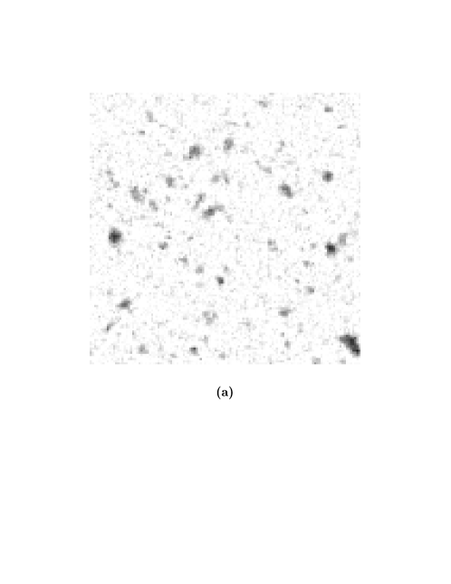
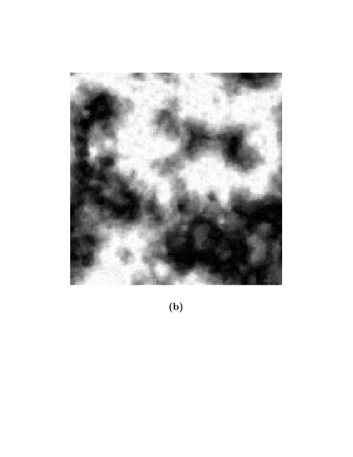
Figure 4: Configurations of the local order parameter $Q_{i}$ at $T\!=\!0.8T_{\rm c}$ and $H_{0}\!=\!0.3J$ for $L\!=\!128$. (a) $\Theta\!=\!0.27<\Theta_{\rm c}$ (dynamically ordered phase). (b) $\Theta\!=\!0.98\!\approx\!\Theta_{\rm c}$ (near the DPT). (c) $\Theta\!=\!2.7>\Theta_{\rm c}$ (dynamically disordered phase). (d) $\Theta\!=\!13.4\!\gg\!\Theta_{\rm c}$ (deeper in the disordered phase). On the gray-scale $-1$ $(+1)$ corresponds to black (white)

Figure 5: Finite-size behavior of our observables at $T\!=\!0.8T_{\rm c}$ and $H_{0}\!=\!0.3J$ for various system sizes. (a) The order parameter $\langle|Q|\rangle_{L}$. (b) The scaled variance $X_{L}$ as defined in (13). (c) The fourth-order cumulant ratio as defined in (14)

Figure 6: Finite-size scaling plots at $T\!=\!0.8T_{\rm c}$ and $H_{0}\!=\!0.3J$ using the two-dimensional Ising exponents: (a) For the order parameter $\langle|Q|\rangle_{L}$. (b) For the scaled variance $X_{L}$. Finite-size scaling plots at the same temperature and field using the random-percolation exponents: (c) For the order parameter $\langle|Q|\rangle_{L}$. (d) For the scaled variance $X_{L}$. The straight lines in all graphs represent the asymptotic large-argument behaviors of the functions ${\cal F}_{\pm}$ and ${\cal G}_{\pm}$ given in (4) and (4), respectively. The value for the (infinite-system) $\Theta_{c}$, used in all four graphs, was obtained from the cumulant crossing [(14)] Fig. 5(c)

References

- [1] Ewing J. A. (1881) Proc. R. Soc. London 33, 21
- [2] Warburg E. (1881) Annalen der Physik und Chemie (Neue Folge) 13, 141
- [3] Ewing J. A. (1882) Proc. R. Soc. London 34, 39
- [4] Steinmetz C. P. (1892) Trans. Am. Inst. Electr. Eng. 9, 3
- [5] Kline R. R. (1992) Steinmetz: Engineer and Socialist. Johns Hopkins University Press, Baltimore
- [6] He Y.-L., Wang G.-C. (1993) Phys. Rev. Lett. 70, 2336
- [7] Jiang Q., Yang H.-N., Wang G.-C. (1995) Phys. Rev. B 52, 14911
- [8] Jiang Q., Yang H.-N., Wang G.-C. (1996) J. Appl. Phys. 79, 5122
- [9] Suen J. H., Erskine J. L. (1997) Phys. Rev. Lett. 78, 3567
- [10] Suen J. H., Lee M. H., Teeter G., Erskine J. L. (1999) Phys. Rev. B 59, 4249
- [11] Jung P., Gray G., Roy R., Mandel P. (1990) Phys. Rev. Lett. 65, 1873
- [12] Rao M., Krishnamurthy H. R., Pandit R. (1990) Phys. Rev. B 42, 856
- [13] Thomas P. B., Dhar D. (1993) J. Phys. A 26, 3973
- [14] Luse C. N., Zangwill A. (1994) Phys. Rev. E 50, 224
- [15] Beale P. D. (1994) Integrated Ferroelectrics 4, 107
- [16] Sides S. W., Rikvold P. A., Novotny M. A. (1998) J. Appl. Phys. 83, 6494
- [17] Sides S. W., Rikvold P. A., Novotny M. A. (1999) Phys. Rev. E 59, 2710
- [18] Tomé T., de Oliveira M. J. (1990) Phys. Rev. A 41, 4251. These authors used the Kubo-Suzuki equation of motion corresponding to the Curie-Weiss form of the bistable free energy. However, equivalent results are obtained from a simple potential.
- [19] Lo W. S., Pelcovits R. A. (1990) Phys. Rev. A 42, 7471
- [20] Acharyya M., Chakrabarti B. (1995) Phys. Rev. B 52, 6550
- [21] Acharyya M. (1997) Phys. Rev. E 56, 1234
- [22] Acharyya M. (1997) Phys. Rev. E 56, 2407
- [23] Acharyya M. (1998) Phys. Rev. E 58, 179
- [24] Sides S. W., Rikvold P. A., Novotny M. A. (1998) Phys. Rev. Lett. 81, 834
- [25] Buendía G. M., Machado E. (1998) Phys. Rev. E 58, 1260
- [26] Acharyya M., Chakrabarti B. K. (1994) In: Stauffer, D. (Ed.) Annual Reviews of Computational Physics I. World Scientific, Singapore, 107
- [27] Chakrabarti B., Acharyya M. (1999) Rev. Mod. Phys. 71, April
- [28] Binder K., Heermann D. W. (1997) Monte Carlo Simulation in Statistical Physics. An Introduction, 3rd edn. Springer, Berlin
- [29] Lubachevsky B. D. (1987) Complex Systems 1, 1099
- [30] Lubachevsky B. D. (1988) J. Comput. Phys. 75, 103
- [31] Korniss G., Brown G., Novotny M. A., Rikvold P. A. Preprint cond-mat/9803118, to appear in Computer Simulation Studies in Condensed Matter Physics XI, edited by D. P. Landau and H.-B. Schüttler. Springer, Berlin
- [32] Korniss G., Novotny M. A., Rikvold P. A. (1998) Preprint cond-mat/9812344, submitted to J. Comput. Phys.
- [33] Rikvold P. A., Tomita H., Miyashita S., Sides S. W. (1994) Phys. Rev. E 49, 5080
- [34] Gunton J. D., San Miguel M., Sahni P. S. (1983) In: Domb C., Lebowitz J. L. (Eds.) Phase Transitions and Critical Phenomena Vol. 8. Academic, New York
- [35] Rikvold P. A., Gorman B. M. (1994) In: Stauffer, D. (Ed.) Annual Reviews of Computational Physics I. World Scientific, Singapore, 149
- [36] Avrami M. (1939) J. Chem. Phys. 7, 1103; (1940) J. Chem. Phys. 8, 212; (1941) J. Chem. Phys. 9, 177
- [37] Ramos R. A., Rikvold P. A., Novotny M. A. (1999) Phys. Rev. B 59, 9053
- [38] Sides S. W., Rikvold P. A., Novotny M. A. (1998) Phys. Rev. E 57, 6512
- [39] Binder K. (1990) In: Privman V. (Ed.) Finite-Size Scaling and Numerical Simulation of Statistical Systems. World Scientific, Singapore, 173
- [40] Landau D. P. (1976) Phys. Rev. B 13, 2997; (1990) In: Privman V. (Ed.) Finite-Size Scaling and Numerical Simulation of Statistical Systems. World Scientific, Singapore, 225
- [41] Stauffer D., Aharony A. (1992) Introduction to Percolation Theory, 2nd edn. Taylor & Francis, London
- [42] Sides S. W., Rikvold P. A., Novotny M. A. (unpublished)
- [43] Kamieniarz G., Blöte H. (1993) J. Phys. A 26, 201