A systematic approach to bicontinuous cubic phases in ternary amphiphilic systems

Abstract

The Fourier approach and theories of space groups and color symmetries are used to systematically generate and compare bicontinuous cubic structures in the framework of a Ginzburg-Landau model for ternary amphiphilic systems. Both single and double structures are investigated; they correspond to systems with one or two monolayers in a unit cell, respectively. We show how and why single structures can be made to approach triply periodic minimal surfaces very closely, and give improved nodal approximations for G, D, I-WP and P surfaces. We demonstrate that the relative stability of the single structures can be calculated from the geometrical properties of their interfaces only. The single gyroid G turns out to be the most stable bicontinuous cubic phase since it has the smallest porosity. The representations are used to calculate distributions of the Gaussian curvature and ${}^{2}H$-NMR bandshapes for C(P), C(D), S, C(Y) and F-RD surfaces.

I Introduction

Amphiphiles are molecules which have both hydrophilic and hydrophobic parts. In a ternary mixture of amphiphiles, water and oil, their ability to stabilize water-oil interfaces leads to structure formation on the nanometer scale [2, 3, 4]. Depending on concentration and temperature, many different phases are found to be stable. One intriguing aspect of amphiphilic polymorphism is the existence of ordered bicontinuous phases which can be traversed in any direction in both the water and the oil regions. Here macroscopic order has been demonstrated by the appearance of Bragg-peaks in diffraction patterns [5] and bicontinuity by measuring diffusion properties with nuclear magnetic resonance [6]. Clearly any bicontinuous ordered phase has to have a three-dimensional Bravais-lattice. In experiments, cubic symmetry is observed in most cases [7, 8, 9]. The amphiphilic monolayers of bicontinuous cubic structures, which separate regions with water from regions with oil, are often modelled by triply periodic surfaces of constant mean curvature [10, 11]. By changing experimental parameters like temperature or salt concentration, their preference to bend towards the water or the oil regions can be made to vanish. Then one can describe them by triply periodic minimal surfaces (TPMS). Similarly, the bilayers of bicontinuous cubic phases in lipid-water mixtures by symmetry have no spontaneous curvature, so that their mid-surfaces can also be modelled by TPMS [12]. Bicontinuous cubic phases have gained renewed interest recently, for example as space partitioners in biological systems [13], as amphiphilic templates for mesoporous systems [14] and for the crystallization of membrane proteins [15].

In this paper, we report on a systematic theoretical investigation of bicontinuous cubic phases in ternary amphiphilic systems with vanishing spontaneous curvature. We restrict ourselves to bicontinuous ordered phases with cubic symmetry since these are the ones which are mainly observed in experiments. It has been shown recently by Góźdź and Hołyst [16] in the framework of real-space minimization that various cubic bicontinuous phases can be generated as local minima of the Ginzburg-Landau model for ternary amphiphilic systems introduced previously by Gompper and Schick [17, 3]. The position of the interfaces between oil and water regions then follow as iso-surfaces to a scalar field $\Phi(\textbf{r})$. Our analysis is based on the Fourier ansatz in combination with the theories of space groups and color symmetries; it allows to generate the relevant structures in a very systematic way and to reduce the representations to a relatively small number of variables. This in turn allows very efficient numerics and makes it easy to document and reuse the results.

In order to analyze our results, we use an effective interface Hamiltonian, which is derived from the Ginzburg-Landau theory [18]. Due to the oil-water symmetry of the Ginzburg-Landau model, the spontaneous curvature vanishes. Since the elastic energy of interfaces is governed by their bending rigidity, the interfaces of the structures which have only one amphiphilic monolayer are very close to cubic TPMS. A similar approach, which employs a Ginzburg-Landau model for binary fluid mixtures, has been used in Refs. [19, 20]. However, since the elastic energy of interfaces is governed by their tension in this case, the numerical minimization is much less stable. In fact, our tabulation of the first few Fourier amplitudes for the four best-known structures G, D, I-WP and P provides a considerable improvement over the widely used nodal approximations for TPMS [21]. Since most of the detailed analysis of the properties of cubic TPMS has been focused on these structures so far, we want to use our representations to characterize the structures C(P), C(D), S, C(Y) and F-RD in more detail.

Our analysis in terms of interfacial properties also allows us to investigate the relative stability of the various bicontinuous cubic phases in terms of their geometrical properties. Although the identification of a certain bicontinuous cubic structure is a tedious procedure best accomplished by combining several experimental techniques like neutron or X-ray small angle scattering, transmission electron microscopy and nuclear magnetic resonance, in most cases one has found the stable phases to be either gyroid or diamond structures. Here we derive an universal geometrical criterion for their relative stability in the case of vanishing spontaneous curvature of the interfaces which explains these experimental findings and is in excellent agreement with our numerical results.

The paper is organized as follows. We begin by introducing the relevant concepts from differential geometry and crystallography and their applications to amphiphilic systems in Sec. II. In Sec. III we explain how to construct Fourier series and nodal approximations for amphiphilic structures. In Sec. IV we systematically generate, evaluate and compare various single and double structures by using the Ginzburg-Landau theory, as well as the interface Hamiltonian which follows from it. In Sec. V we use the representations obtained to comment on the experimental identification of bicontinuous cubic phases in amphiphilic and mesoporous systems.

II Geometry of bicontinuous phases

If we characterize a bicontinuous phase by its interfaces, the simplest possible case is that they form one triply periodic surface (TPS), i.e. a surface with a three-dimensional Bravais-lattice. Any TPS divides space into two unconnected but intertwined labyrinths. In ternary amphiphilic systems, the surface is covered with an amphiphilic monolayer and the two labyrinths are filled with water and oil, respectively. Therefore any structure corresponding to a TPS is bicontinuous in water and oil. The TPS is called balanced if there exists an Euclidean transformation $\alpha$ which maps one labyrinth onto the other. Oil and water have equal volume fractions in this case.

In the mathematical context, triply periodic minimal surfaces (TPMS) have been investigated extensively [22, 23]. In order to locally minimize their surface area, minimal surfaces have vanishing mean curvature $H=(1/R_{1}+1/R_{2})/2$ at every point on the surface, where $R_{1}$ and $R_{2}$ are the two principal radii of curvature. Therefore, their Gaussian curvature $K=1/R_{1}R_{2}=-1/R_{1}^{2}$ is non-positive and the surface is saddle-shaped everywhere. Up to 1970 only five TPMS had been known by the 19th-century work of Schwarz and his students, with P, D and C(P) being cubic. Then Schoen described 12 more [24], including the cubic cases G, F-RD, I-WP, O,C-TO and C(D). Their existence was proven by Karcher in 1989 [25]. More TPMS have been found by Karcher and Polthier [26], Fischer and Koch [27] and others, but all of them seem to be more complicated than the ones known to Schoen. For cubic TPMS, exact representations are known only for P, D, G and I-WP. These Weierstrass representations originate from complex analysis and are explained in Appendix A. With their help the surface areas of these TPMS can be calculated exactly in terms of elliptic functions; the resulting values are given in Tab. I.

Being balanced and being minimal are two independent possible properties of a TPS. From the cubic TPMS known to Schoen, F-RD, I-WP and O,C-TO are not balanced and divide space into two labyrinths with unequal volume fractions. On the other hand, the TPS defined by $\cos x+\cos y+\cos z=0$ is balanced with $\alpha$ being a translation along half the body diagonal of the conventional unit cell, but far from minimal. If a TPS contains straight lines, it is called spanning [28]. It was shown by Schwarz that any spanning TPMS is symmetric with respect to a reflection around such a line. Since this operation exchanges the two labyrinths, any spanning TPMS is balanced. The only known cubic TPMS, which is balanced but not spanning, is the gyroid G, where the symmetry operation exchanging the two labyrinths is the inversion.

For our purposes it is best to investigate not the local concentrations of oil and water separately, but their difference $\Phi(\textbf{r})=\rho_{O}(\textbf{r})-\rho_{W}(\textbf{r})$. Since we assume incompressibility, $\rho_{O}(\textbf{r})+\rho_{W}(\textbf{r})=1$ and the local concentrations of oil and water can be reconstructed from $\Phi(\textbf{r})$. The amphiphilic monolayers now correspond to the $\Phi=0$ iso-surfaces. The interchange of oil and water amounts to $\Phi\to-\Phi$. For balanced surfaces this is a symmetry operation when combined with the Euclidean operation $\alpha$, that is $\Phi(\alpha\textbf{r})=-\Phi(\textbf{r})$. However, it is important to note that this is not a space group symmetry — which would only allow for a rigid motion, but not for a change of sign. Additional symmetries which arise when an Euclidean operation is combined with a permutation are called color symmetries; with only water and oil present we have the simplest case of a black and white symmetry [29, 30, 31]. When water and oil are colored white and black, respectively, the $\Phi=0$ iso-surface obtains differently colored sides and thus can be considered to be oriented. We assume the uncolored structure (i.e. the unoriented surface) to have space group ${\cal G}$. Then all Euclidean operations which do not interchange the two labyrinths form a subgroup ${\cal H}$ of ${\cal G}$ of index $2$. By definition ${\cal H}$ is the space group of the colored structure (i.e. the oriented surface). The quotient group is isomorphic to the cyclic group of order $2$, that is ${\cal G}/{\cal H}\cong{\mathbb{Z}}_{2}\cong\{1,\alpha\}$. In general, any balanced TPS is characterized by a group-subgroup pair ${\cal G}-{\cal H}$ of index $2$. For example, for the balanced TPS defined by $\cos x+\cos y+\cos z=0$, we have ${\cal H}=Pm\bar{3}m$ (No. 221) and ${\cal G}=Im\bar{3}m$ (No. 229).

In order to describe a balanced TPS which does not intersect itself, certain restrictions apply for the extension from ${\cal H}$ to ${\cal G}$ (for example, if $\alpha$ is a rotation, it has to be 2-fold). This has been used by Fischer and Koch to develop a crystallographic classification of all cubic TPMS [28, 27]. In particular they showed that only 34 cubic group-subgroup pairs ${\cal G}-{\cal H}$ with index 2 can correspond to cubic balanced TPMS. Although there is no way to systematically list all balanced TPMS belonging to a possible group-subgroup pairing ${\cal G}-{\cal H}$, Fischer and Koch argued that one can completely enumerate all cubic spanning TPMS which have straight lines forming a three-dimensional network whose polygons are spanned disc-like by the surface. They find P, C(P), D, C(D), S and C(Y), with the latter two described by them for the first time. In our work we systematically generate these structures together with the only known balanced but non-spanning cubic TPMS G and the non-balanced ones I-WP and F-RD. Examples for spanning TPMS are shown in Fig. 1.

One also can consider structures with two TPS. For example, parallel surfaces can be constructed on either side of any given TPS. Both parallel surfaces are TPS, each of which has two labyrinths, which are topologically equivalent to those of the initial structure. However, with respect to the overall structure, these labyrinths are now filled with the same component and separated by a bilayer which is filled with the other component. One might call this structure tricontinuous, but we rather prefer to use the term double structures for structures of two TPS — in contrast to single structures containing one TPS.

Experimentally, little is known about the exact structure of bicontinuous cubic phases in ternary amphiphilic systems. One exception is the system DDAB-water-styrene, for which five different double structures have been found to be stable, each of which can be regarded as an oil-filled bilayer draped onto a different TPS [32]. However, with microemulsion phases being so ubiquitous for these systems, single structures can be expected also to be stable, and in fact have been reported in Ref. [33]. In contrast to the situation for (almost balanced) ternary amphiphilic systems, the structure of bicontinuous cubic phases is well-established for many binary amphiphilic systems [7, 8, 9]. Here, mostly inverse phases are found, in which the two labyrinths are filled with water and the TPS is covered with an amphiphilic bilayer. These structures can be considered to be double structures of a ternary system where the oil has been removed from the bilayer. However, if the thickness of the bilayer is small compared to the lattice constant, it seems more appropriate to model them by single structures of a ternary system, where the water regions on both sides of the bilayer are distinguished artificially by labelling them ‘water I’ and ‘water II’, respectively [34]. Thus our results for single structures can also be applied to bicontinuous cubic phases in amphiphile-water mixtures.

III Fourier ansatz

In order to construct a Fourier ansatz for a given group-subgroup pair ${\cal G}-{\cal H}$, we need a Fourier ansatz for space group ${\cal H}$, together with the implementation of a certain black and white symmetry. In ternary amphiphilic systems, this corresponds to a balanced single structure. For non-balanced single structures and double structures there is no color symmetry and one only needs the Fourier ansatz for a given space group ${\cal H}\equiv{\cal G}$.

It is well known how to choose the Fourier ansatz for a given space group ${\cal H}$ [35, 36]. In the cubic system the translational properties of ${\cal H}$ correspond to one of the three cubic Bravais lattices simple cubic (P), body centered cubic (I) or face centered cubic (F). The Fourier series then reads

$$\Phi(\textbf{r})=\sum_{\{\textbf{K}\}}\Phi_{\textbf{K}}\ e^{i\textbf{K}\cdot\textbf{r}}\$$ (1)

where $\{\textbf{K}\}$ is the reciprocal lattice and the $\Phi_{\textbf{K}}$ are the (complex) Fourier amplitudes. However, not all of them are independent. Since the density field $\Phi(\textbf{r})$ has to be real, it follows from Eq. (1) that $\overline{\Phi_{\textbf{K}}}=\Phi_{-\textbf{K}}$. With $\Phi_{\textbf{K}}=A_{\textbf{K}}-iB_{\textbf{K}}$ , Eq. (1) becomes

$$\Phi(\textbf{r})=\sum_{\{\textbf{K}\}}\left\{A_{\textbf{K}}\cos(\textbf{K}\cdot\textbf{r})+B_{\textbf{K}}\sin(\textbf{K}\cdot\textbf{r})\right\}\ .$$ (2)

Here $A_{\textbf{K}}$ and $B_{\textbf{K}}$ are real and can be obtained from $\Phi(\textbf{r})$ as

$$A_{\textbf{K}}=\frac{1}{v}\int d\textbf{r}\ \Phi(\textbf{r})\ \cos(\textbf{K}\cdot\textbf{r}),\ \ \ \ \ \ B_{\textbf{K}}=\frac{1}{v}\int d\textbf{r}\ \Phi(\textbf{r})\ \sin(\textbf{K}\cdot\textbf{r}),$$ (3)

where the integration runs over some unit cell of volume $v$. Thus, for even or odd functions, $B_{\textbf{K}}=0$ or $A_{\textbf{K}}=0$, respectively.

Further restrictions on the Fourier amplitudes $\Phi_{\textbf{K}}$ arise when we consider symmetry operations $\textbf{r}\to P\textbf{r}+\textbf{t}$, which are not pure translations. Here, $P$ denotes a rotation, inversion or roto-inversion, and t a translation which does not belong to the Bravais lattice. Thus, t is non-vanishing for screw axes and glide planes. It now follows from Eq. (1) that $\Phi_{P^{-1}\textbf{K}}=\Phi_{\textbf{K}}\ e^{i\textbf{K}\cdot\textbf{t}}$. Let $H$ be the point group of the given space group ${\cal H}$. To each operation in $H$ there corresponds a pair $(P,\textbf{t})$ in ${\cal H}$. We group all reciprocal lattice vectors, which are related by an operation of $H$, into so-called Fourier stars. All members of a given star have the same wavelength. Only few stars will have the same wavelength and in most cases there is only one star with a certain wavelength. Therefore, the stars can be ordered according to decreasing wavelength and numbered with the index $i$. For each star we arbitrarily choose one representative $\textbf{K}_{i}$. With $\Phi_{\textbf{K}_{i}}=A_{i}-iB_{i}$, Eq. (1) becomes a sum over Fourier stars,

$$\Phi(\textbf{r})=\sum_{i}\frac{n_{i}}{n}\ \{A_{i}\ {\cal A}_{\textbf{K}_{i}}(\textbf{r})+B_{i}\ {\cal B}_{\textbf{K}_{i}}(\textbf{r})\}\ ,$$ (4)

where the geometric structure factors are defined by

$${\cal A}_{\textbf{K}_{i}}(\textbf{r}) = \sum_{H}\cos[(P^{-1}\textbf{K}_{i})\cdot\textbf{r}+\textbf{K}_{i}\cdot\textbf{t}],$$ (5)

$${\cal B}_{\textbf{K}_{i}}(\textbf{r}) = \sum_{H}\sin[(P^{-1}\textbf{K}_{i})\cdot\textbf{r}+\textbf{K}_{i}\cdot\textbf{t}]\ .$$ (6)

Their precise form is obtained by explicitly enumerating all non-translational symmetry operations of space group ${\cal H}$. The results of this procedure can be taken from Ref. [35] if they are corrected by a factor $1/m_{L}$, where $m_{L}$ is the multiplicity of the Bravais lattice (1, 2 and 4 for P, I and F, respectively). In Eq. (4), $n$ denotes the order of $H$ and $n_{i}$ the multiplicity of $\textbf{K}_{i}$. If $H$ does not contain the inversion, we can extend the definition of a Fourier star by using $\overline{\Phi_{\textbf{K}}}=\Phi_{-\textbf{K}}$. This does not change Eq. (4) except that now we have to replace $H$ by the so-called Laue group, that is $H$ extended by the inversion. All structures investigated in this work have $m\bar{3}m$ with order $n=48$ either as their point group or as their Laue group, thus the members of one star are generated by all possible permutations and changes of sign of the components of $\textbf{K}_{i}$. With $A_{i}=A_{\textbf{K}_{i}}$ and $B_{i}=B_{\textbf{K}_{i}}$, every Fourier star has two variables. This reduces to one when $\Phi$ is an even or odd function of r.

We now address the question how to implement the additional black and white symmetry. Since ${\cal H}$ has index $2$ in ${\cal G}$, it follows from the theorem of Hermann [30] that ${\cal H}$ has either the same point group or the same Bravais lattice as ${\cal G}$. If ${\cal H}$ and ${\cal G}$ have the same point group, their Bravais lattices have to be different. Thus the Euclidean operation $\alpha$, which maps oil regions onto water regions, has to be a translation $\textbf{t}_{\alpha}$ which transforms one cubic Bravais-lattice into another. There are only two possibilities: for $\textbf{t}_{\alpha}=a(\textbf{x}+\textbf{y}+\textbf{z})/2$ a P-lattice becomes a I-lattice, and for $\textbf{t}_{\alpha}=a\textbf{x}/2$ a F-lattice becomes a P-lattice. The operation $\Phi(\textbf{r}+\textbf{t}_{\alpha})=-\Phi(\textbf{r})$ in combination with Eq. (1) leads to additional reflection conditions: $h+k+l=2n+1$ for $P\to I$, and $h,k,l=2n+1$ for $F\to P$. Note that these reflection conditions are complementary to the well-known ones for I and F ($h+k+l=2n$ and $h+k,h+l,k+l=2n$, respectively). Thus in the case of identical point groups, the form of the Fourier stars in Eq. (4) for space group ${\cal H}$ stays the same, but the sum now runs over a reduced set of Fourier stars.

If ${\cal H}$ and ${\cal G}$ have the same Bravais lattice, their point groups have to be different. Thus the Euclidean operation $\alpha$ has to be a point group operation $P_{\alpha}$ which extends one cubic point group into another one. There are five cubic point groups and six ways to extend one of them into another by some $P_{\alpha}$. From $\Phi(P_{\alpha}\textbf{r})=-\Phi(\textbf{r})$ and Eq. (1) we now find $\Phi_{P_{\alpha}^{-1}\textbf{K}}=-\Phi_{\textbf{K}}\exp(i\textbf{K}\cdot\textbf{t}_{\alpha})$. Thus, different Fourier stars merge to form new ones. However, in all cases considered in this work there is no need to consider new Fourier stars, since we only deal with the simple case that $P_{\alpha}$ is the inversion. Then $\textbf{t}_{\alpha}=\textbf{0}$ and one finds $A_{i}=0$ for all $i$. The same result of course follows from Eq. (2), since now $\Phi$ is an odd function of r.

Tab. II lists the group-subgroup pairs ${\cal G}-{\cal H}$ and the nature of the extension ${\cal H}\to{\cal G}$ for the nine single structures investigated in this paper [28, 27]. Out of the seven balanced cases, five have identical point groups and two have identical Bravais lattices with $P_{\alpha}$ being the inversion. In the next section, we will discuss our numerical results for Fourier series of functions $\Phi(\textbf{r})$, whose $\Phi=0$ iso-surfaces approximate triply periodic minimal surfaces. However, a very simple approximation can be obtained by only considering the space group information. The use of a single Fourier star leads to the so-called nodal approximation, which does not need any Fourier amplitude. For balanced structures, it is essential to consider the correct black-and-white symmetry. If one Fourier star is not sufficient to represent the topology correctly, one has to consider another one and adjust its Fourier amplitude by visual inspection. In the last column of Tab. II, nodal approximations are given for the nine single structures investigated. They have been derived in the context of triply periodic zero potential surfaces of ionic crystals [21] and are widely used as approximations for TPMS (e.g. in Refs. [13, 37]). However, it is well known that their properties can differ considerably from those of real TPMS [38]. In the next section we will show that the quality of the nodal approximation varies considerably for different structures.

IV Triply periodic structures in Ginzburg-Landau models

A Ginzburg-Landau model

The simplest Ginzburg-Landau model [17], which successfully describes the phase behavior and mesoscopic structure of ternary amphiphilic systems, contains a single, scalar order parameter field $\Phi(\textbf{r})$; thus, amphiphilic degrees of freedom are integrated out. The model is defined by the free-energy functional

$${\cal F}[\Phi]=\int\ d\textbf{r}\ \left\{(\Delta\Phi)^{2}+g(\Phi)(\nabla\Phi)^{2}+f(\Phi)\right\}\ .$$ (7)

For ternary amphiphilic systems at the phase inversion temperature, the free-energy functional has to be symmetrical in water and oil, i.e. invariant under the transformation $\Phi\to-\Phi$. A convenient form for the free-energy density and the structural parameter of the homogeneous phases are [39]

$$f(\Phi)=(\Phi+1)^{2}(\Phi-1)^{2}(\Phi^{2}+f_{0})\ ,\ \ \ \ \ \ g(\Phi)=g_{0}+g_{2}\Phi^{2}\ .$$ (8)

Here, the three minima at $-1$, $0$ and $1$ correspond to excess water, microemulsion and excess oil phases, respectively, and $f_{0}$ acts as a chemical potential for amphiphiles. The behavior of the correlation function $\langle\Phi({\bf r}_{1})\Phi({\bf r}_{2})\rangle$ is controlled by the parameters $g_{0}$ and $g_{2}$ in the microemulsion and excess phases, respectively; they are therefore related to the amphiphilic strength and the solubility of the amphiphile [3]. Strongly structured microemulsions are obtained for $g_{0}<0$, while unstructured excess phases require $(g_{2}+g_{0})$ to be positive and sufficiently large.

The elastic properties of amphiphilic monolayers are described by the Canham-Helfrich Hamiltonian [40, 41]

$${\cal H}=\int dA\ \left\{\sigma+2\kappa\ (H-c_{0})^{2}+\bar{\kappa}\ K\right\}\ ,$$ (9)

where the integration extends over the surface, $H$ and $K$ are mean and Gaussian curvature, respectively, and the elastic moduli are the surface tension $\sigma$, the spontaneous curvature $c_{0}$, the bending rigidity $\kappa$ and the saddle-splay modulus $\bar{\kappa}$. If the $\Phi=0$ iso-surfaces are identified with the location of the amphiphilic monolayers, the free energy of the Ginzburg-Landau model (7) can be well approximated by a sum of the curvature energy — calculated from Eq. (9) — and a direct interaction between the interfaces, which falls off exponentially with distance [18, 39]. Due to the water-oil symmetry the spontaneous curvature $c_{0}$ vanishes. The values of the other elastic moduli can be calculated numerically from the profile $\Phi_{s}(z)$, which minimizes the free energy of a planar water-oil interface [18].

With $f_{0}$, $g_{0}$ and $g_{2}$, the model has a three-dimensional parameter space. We investigate bicontinuous cubic phases in the mean-field approximation. For $f_{0}<0$ the excess phases W/O are stable, for $f_{0}>0$ the microemulsion ME. Moreover, for sufficiently negative $g_{0}$ and not too large $g_{2}$, a (singly periodic) lamellar phase $L_{\alpha}$ is found to be stable. Fig. 2 shows cuts through the parameter space for $g_{0}=-3.0$ and $g_{0}=-4.5$. At each point of parameter space, the elastic moduli can be determined numerically. In the region where $\sigma<0$, the system gains free energy by forming interfaces; the lamellar phase is stabilized by the short-ranged, repulsive part of the interaction between them. In the vicinity of the $\sigma=0$-line with $\sigma>0$, the lamellar phase still exists — stabilized by the long-ranged, attractive part of the interaction between interfaces. However, for a given $g_{0}$ there is exactly one point where the phase boundary and the $\sigma=0$-line touch each other [42]. Here the interaction between lamellae vanishes and their distance diverges. We call this point unbinding point since this divergence resembles a continuous unbinding transition [43, 44]. We will later make use of the fact that in the vicinity of the unbinding point the free energy of the Ginzburg-Landau model (7) is dominated by its interfacial contributions. To our knowledge, no other phases are stable in the Ginzburg-Landau model. The (doubly periodic) hexagonal phase as well as the (triply periodic) cubic phases investigated below are only metastable. If one raises $g_{0}$ to $g_{0}=-2$, the lamellar channel vanishes, and microemulsion and excess phases coexist for $f_{0}=0$ and large $g_{2}$. As $g_{0}$ approaches zero from below (with $g_{2}>0$), the lamellar phase disappears.

B Generating triply periodic structures

In order to generate the structures described in Sec. II as local minima of the Ginzburg-Landau functional, we construct the Fourier series for the corresponding space group pair (listed in Tab. II), as described in Sec. III, and terminate it after $N$ stars. For a given set of parameters $(f_{0},g_{0},g_{2})$, the free-energy functional (7) becomes a function of the Fourier amplitudes $A_{i}$ and $B_{i}$ $(1\leq i\leq N)$, the constant mode $A_{0}$ and the lattice constant $a$. Although the integral in Eq. (7) could be solved exactly by using the orthogonality of trigonometric functions, we use Gaussian integration which is equivalent in efficiency and accuracy, but easier to implement. For minimization we use conjugate gradients and as initial profile the nodal approximations given in Tab. II. Note that certain structures like P and C(P) need the same Fourier ansatz but different initial profiles. In order to obtain initial profiles for the double structures, we transform the nodal approximations of the corresponding single structures according to $\Phi\to 2\Phi^{2}-1$ in real space and then transform these profiles to Fourier space by using Eq. (3). In order to test for convergence of the Fourier series, we increase $N$ successively and require both the values for the free-energy density $f$ and the lattice constant $a$ to level off. With a typical workstation $N\approx 100$ is feasible, but $N\approx 30$ turns out to be sufficient in most cases. If a profile has converged, the Fourier amplitudes fall off exponentially for large $|\textbf{K}_{i}|$.

We have generated the nine single structures discussed in Sec. II and the double structures corresponding to the four most relevant single structures. In Fig. 3 we visualize single and double structures of P, D, G and I-WP by drawing their $\Phi=0$ iso-surfaces in a conventional unit cell. The two interfaces of the double structures form a bilayer wrapped onto the interfaces of the single structures. For $f_{0}=0.0$, $g_{0}=-3.0$ and $g_{2}=7.01$ our numerical results are summarized in Tab. III. This point is chosen here in order to compare our results with those of Góźdź and Hołyst [16]. For each structure, we give the free energy density $f$, the lattice constant $a$ and the volume fraction of oil $v=1/V\int d\textbf{r}(\Phi(\textbf{r})+1)/2$. The structures are ordered with respect to their free-energy density $f$; thus, for the single structures we find the hierarchy G - S - D - I-WP - P etc. The scaled surface area $A/a^{2}$ and the Euler characteristic $\chi$ are calculated for the conventional unit cell by triangulating the $\Phi=0$ iso-surface with the marching cube algorithm. By successively refining the discretization, we calculate the sum $A_{M}$ over the surface areas of the triangles as a function of their number $M$, and then extrapolate to $A=A_{\infty}$ by fitting $A_{M}$ to a linear $1/M$-dependence. The values obtained for P, D, G and I-WP turn out to be very close to the ones for the corresponding minimal surfaces as calculated from the Weierstrass representations and given in Tab. I. The Euler characteristic $\chi$ can be calculated as $\chi=C-E/4$ where C is the number of cubes and E is the number of cube edges cut by the surface. All our numerical results agree very well with those reported by Góźdź and Hołyst in Ref. [16] for G, D, P and I-WP.

In order to evaluate the curvature properties of the $\Phi=0$ iso-surfaces, we make use of the fact that — due to the Fourier ansatz — the field $\Phi(\textbf{r})$ is known analytically. The mean and Gaussian curvatures, [45, 38]

$$H=-\frac{1}{2}\ \nabla\cdot\textbf{n}\ ,\quad K=\frac{1}{2}\ \left[(\nabla\cdot\textbf{n})^{2}-\sum_{i,j=1}^{3}\ \partial_{i}n_{j}\ \partial_{i}n_{j}\right]\ ,$$ (10)

where $\textbf{n}=\nabla\Phi/|\nabla\Phi|$ is the surface normal vector, can then be calculated exactly. In Fig. 4 we plot the distribution of $H$ and $K$ over the $\Phi=0$ iso-surface as histograms for the structures P, D, G and I-WP in a conventional unit cell. Numerical inaccuracies arise here only from the calculation of the position vectors of the $\Phi=0$ iso-surface with the marching cube algorithm, and from the triangle areas $\Delta A_{i}$, which enter as weighting factors of $H$ and $K$ for each plaquette of the triangulation. The mean curvature is close to zero everywhere. For the balanced structures P, D and G it is distributed symmetrically around $H=0$. We conclude that the $\Phi=0$ iso-surfaces of our numerical solutions are very close, but not identical to the corresponding TPMS. For the Gaussian curvature, we also plot the distribution obtained from the Weierstrass representation by numerically evaluating Eq. (A3). This is done by evaluating $K(x+iy)$ on a square lattice in $x$ and $y$, which covers the fundamental domains for P, D, G and I-WP as given in Appendix A, and collect the values in a histogram with weights $dA(x+iy)$. The resulting distributions of $K$ are scaled to unit lattice constant by using the Weierstrass lattice constants given in Tab. I, and normalized to $\int dKp(K)=1$. For P, D and G, these distributions $p(K)$ are identical (apart from the scale) since they are related to each other by a Bonnet transformation. Fig. 4 shows that the numerical distributions agree very well with the exact Weierstrass results. The surface area is not very sensitive to the detailed shape of the interfaces in these cases; the values for the full solutions and the nodal approximations differ only by a few percent. Finally, we can test the procedure used here by employing the Gauss-Bonnet theorem to calculate the Euler characteristic as $\chi=1/(2\pi)\int dAK$. We find an agreement to three relevant digits.

The $K$-distributions of the single structures investigated, for which no Weierstrass representations are known, are shown in Fig. 5. These surfaces typically have a more complicated structure within the unit cell, which is reflected in both a larger number of peaks and in a larger extremal value of the Gaussian curvature, $K_{min}$.

The Fourier ansatz yields representations of TPMS which are easy to document and thus straightforward to use in further investigations. In Tab. IV, we give improved nodal approximations which consist of up to six Fourier stars. When the number of Fourier stars $N$ is increased, the free-energy density $f$ decreases monotonically, but the quality of the approximation for the corresponding TPMS does not necessarily improve in the same way. Therefore for each structure we choose an optimal value of $N$. The quality of the approximation is judged from the distribution of $H$ and $K$ over the surface, as described above. In Tab. V, we compare the nodal approximations from Tab. II, the improved nodal approximations from Tab. IV and the exact Weierstrass representations by monitoring $H_{max}$, the maximum of $|H|$ on the iso-surface, $\sqrt{\langle H^{2}\rangle}$, the square of the variance of $H$ on the iso-surface, and $K_{min}$, the minimal value of $K$ on the iso-surface. For the exact Weierstrass representation, one has $H_{max}=\sqrt{\langle H^{2}\rangle}=0$. For the improved nodal approximations, the values for $H_{max}$ and $\sqrt{\langle H^{2}\rangle}$ improve by nearly one order of magnitude when compared with the nodal approximations. Also, their distributions of $K$ are very close to the ones obtained from the Weierstrass representations (the only exception is G, whose nodal approximation is already quite good, in particularly for its $K$-distribution). Thus by adding just a few more modes, we can considerably improve on the widely used nodal approximations. Finally, we want to point out that the values of the amplitudes for P, D and I-WP given in Tab. IV are of the same magnitude as those calculated from the representations for TPMS obtained in Ref. [46]. The different values arise from the different shapes of the order parameter profile through the interface. The Ginzburg-Landau model gives interfaces with a finite width, while the calculation based on TPMS assumes sharp interfaces. In fact, the amplitudes of the Ginzburg-Landau model should approach the sharp-interface results as the unbinding point is approached. As the interface effectively sharpens, the Fourier amplitudes decay more and more slowly as a function of the wave number $|{\bf K}|$, with a $|{\bf K}|^{-2}$ behavior in the limit of step-like interfaces — in agreement with the well-known $|{\bf K}|^{-4}$ Porod-law for the scattering intensity of sharp interfaces [47]. Note that Tab. IV now provides data for G for the first time, which in fact is the cubic bicontinuous phase most relevant for amphiphilic systems [7, 8, 9].

C Hierarchy of structures

In order to investigate the relative stability of the cubic structures in the symmetric Ginzburg-Landau model, we now consider their interfacial properties. For a triply-periodic cubic structure, the free-energy density within the curvature model (9) reads

$$f_{curv}=\frac{1}{a}\left(\sigma A^{*}\right)+\frac{1}{a^{3}}\left(2\kappa\int dA\ H^{2}+2\bar{\kappa}\pi\chi\right)$$ (11)

where $A^{*}=A/a^{2}$ is the scaled area per unit cell; the surface area $A$, the integration of $H^{2}$ and the Euler characteristic $\chi$ once again refer to the conventional unit cell. Both terms in brackets are scale invariant, i.e. they do not depend on the lattice constant $a$. If the elastic moduli are calculated for the points in the phase diagram where we minimize the functional, we find $\sigma<0$, $\kappa>0$ and $\bar{\kappa}<0$. In particular, for $f_{0}=0.0$, $g_{0}=-3.0$ and $g_{2}=7.01$ we obtain $\sigma=-0.84587$, $\kappa=2.36197$ and $\bar{\kappa}=-0.97646$. This explains why the bicontinuous phases cannot be stable in our model. The negative surface tension favors modulated phases, and the bending rigidity favors minimal surfaces; however, only the lamellar phase is not disfavored by the negative saddle-splay modulus. We now also understand why the cubic structures are stable in the Ginzburg-Landau model with respect to a variation of $a$. There is a balance between the negative surface tension term, which favors small values of $a$, and the positive curvature contributions which favor large $a$. The minimization of Eq. (11) with respect to $a$ yields

$$a_{min}=\left(\frac{6\pi\bar{\kappa}\chi+6\kappa\int dAH^{2}}{|\sigma|A^{*}}\right)^{\frac{1}{2}},\quad f_{min}=-\left(\frac{4}{27}\right)^{\frac{1}{2}}\left(\frac{(|\sigma|A^{*})^{3}}{2\bar{\kappa}\pi\chi+2\kappa\int dAH^{2}}\right)^{\frac{1}{2}}\ ,$$ (12)

where $A^{*}$ is assumed to be (approximately) independent of $a$. We can now understand why the single structures are found to be so close to minimal surfaces; the minimum of $\int dAH^{2}$ (the so-called Willmore problem [48]) in this case is $H=0$, which in turn minimizes $f_{min}$. Note that this reasoning is not rigorous, since the minimization of the free-energy functional with respect to lattice constant and shape are not independent; the latter step determines $A/a^{2}$, which is taken to be constant in the first step.

We first discuss the single structures without the “complicated” phases C(P), C(D), S and C(Y) — which have larger lattice constants, a more pronounced modulation within the unit cell, and stronger interactions between the surfaces. Then we numerically find $\int dAH^{2}\approx 10^{-3}$ (compare Fig. 4), so that Eq. (12) becomes

$$a_{min}=\left(\frac{6\pi\bar{\kappa}\chi}{|\sigma|A^{*}}\right)^{\frac{1}{2}},\quad f_{min}=-\left(\frac{4}{27}\right)^{\frac{1}{2}}\ \left(\frac{|\sigma|^{3}}{|\bar{\kappa}|}\right)^{\frac{1}{2}}\ \Gamma$$ (13)

where $\Gamma=({A^{*}}^{3}/2\pi|\chi|)^{\frac{1}{2}}=(A^{3}/2\pi|\chi|a^{6})^{\frac{1}{2}}$ is the topology index. Its exact and numerical values for the single structures investigated is given in Tab. I and Tab. III, respectively. This geometrical quantity is independent both of lattice constant and choice of unit cell. It can be considered to be a measure for the porosity of the structure (the larger its value, the less porous) as well as for the specific surface area (the larger its value, the more surface area per volume). Its relevance for amphiphilic systems is well known [49, 50, 51]. In fact it follows from the isoperimetric relations in three-dimensional space that $A^{3}/|\chi|a^{6}$ is the only invariant combination of Minkowski functionals for vanishing integral mean curvature [52].

A comparison of Eq. (13) with our numerical results from Tab. III shows that these formulae systematically predict a lattice constant and a free-energy density, which are too large and too low by about $20\%$, respectively. However, the hierarchy of structures as predicted by $f_{min}$ turns out to be exactly the same as given in Tab. III by the full numerical results for $f$: G - D - I-WP - P - F-RD. We therefore conclude that the gyroid structure is the most stable structure since it has the smallest porosity (the largest topology index). This corresponds to the fact that topologically the gyroid’s labyrinths have the smallest connectivity of all structures considered — G is the only structure with only three lines meeting at one vertex (D and P have four and six, respectively). With the topology index, we have found a universal geometrical criterion for the relative stability of the various single bicontinuous cubic phases, which also resolves the debate about the degeneracy of minimal surfaces in the Canham-Helfrich approach for vanishing spontaneous curvature. In order to explain the non-degeneracy observed experimentally for binary lipid-water systems, higher order terms [53] and frustration of chain stretching [10, 54] have been considered. In our description both effects are not necessary. In fact, in a (balanced) ternary system, chain stretching does not provide a plausible mechanism for lifting the degeneracy of the free energies of different TPMS, since the presence of oil relieves the frustration in the chain conformations. In the part of the phase diagram, where ordered phases are stable, the free-energy density should contain a negative surface tension contribution (compare Refs. [57, 39]) and the topological term — which due to the Gauss-Bonnet theorem is often neglected, but in fact prevents the lattice constant from shrinking to zero [55]. The same reasoning might be applied to binary systems by identifying monolayers with bilayers and oil and water with water I and water II, respectively. Although the presence of a negative surface tension is essential in our argument, we want to emphasize that its magnitude can still be very small.

There are two main reasons why Eq. (13) yields the correct hierarchy in $f_{min}$, but does not reproduce the numerical values very well. First, by focussing on the interfacial properties, we have neglected the contributions to the free-energy density due to direct interactions between the interfaces, and second, the reasoning leading to Eq. (12) is not rigorous. In order to check whether this is indeed the origin of the numerical discrepancy, we can make use of the existence of the unbinding point in the phase diagram, Fig. 2. At this point, both $\sigma$ and the interaction vanish and the structures investigated should become exactly minimal surfaces. However, at the same point the lattice constant diverges, and both the minimization and the Fourier ansatz become unfeasible. Therefore, we study the approach to the unbinding point along the path shown in Fig. 2. Numerically we find for P, D and G that the deviation of the values for $f$ ($a$) from Eq. (12) relative to our numerical results reduces from $14\%$ ($20\%$) through $11\%$ ($16\%$) to $5\%$ ($7\%$) for the three sets of parameters considered. This demonstrates the convergence towards minimal surfaces, and verifies our reasoning above.

In contrast to the case of “simple” single structures discussed so far, the topology index $\Gamma$ does not predict the hierarchy found numerically for the more complicated single structures C(P), C(D), S and C(Y), compare Tab. III. This may be due to numerical uncertainties in the value of $\Gamma$, since no exact results are available for the surface area $A/a^{2}$. However, both the low Ginzburg-Landau free-energy density and the large topology index of the S-surface indicate that this structure should be comparable in stability with the G-surface. We believe that double structures are not favored in our model because their interfaces are not minimal surfaces, and can be better described as surfaces of constant mean curvature.

One of the intriguing aspects of the Ginzburg-Landau model is that it has a very rugged energy landscape with many local minima. In fact, we were able to find many more interesting structures, including more complicated minimal surfaces and surfaces which contain both saddle-shaped pieces and pieces with positive Gaussian curvature. The latter result is related to the observation that we essentially solve the Willmore problem, which allows for solutions which have both regions with $K>0$ and regions with $K<0$ — for example, the Clifford torus [48].

V Scattering intensities and NMR-spectra

We expect the nine single and four double structures investigated in this paper to include all physically relevant bicontinuous cubic phases in ternary systems near their phase-inversion temperature. The representations of these phases can now be used to simulate data for those experimental techniques, which mainly depend on the geometry of the structures. This includes small angle scattering (SAS), transmission electron microscopy (TEM) and nuclear magnetic resonance (NMR). In particular, our representations can be used to analyze experimental data for mesoporous systems when bicontinuous cubic phases have been used as templates [14].

Since their typical length scales are in the nanometer range, amphiphilic structures can be investigated by X-ray and neutron small angle scattering (SAXS and SANS). The scattering function $S(\textbf{k})$ is obtained from the Fourier transform $\Phi(\textbf{k})$ of the density $\Phi(\textbf{r})$ of scattering lengths as $S(\textbf{k})=|\Phi(\textbf{k})|^{2}$. For SANS, the scattering contrast can be varied by deuterating the sample. For balanced single structures, it is clear from above that with bulk contrast one measures space group ${\cal H}$, with film contrast space group ${\cal G}$. Thus, by varying the contrast in SANS-experiments, the space group pair of the investigated structure can be determined [33, 56]. With our representations of the cubic structures, it is straightforward to calculate the corresponding scattering amplitudes which are needed to analyze the experimental data.

It is quite clear from our results why the program to identify a structure from its scattering intensity alone is rather difficult. For the single structures, the Fourier amplitudes decay so rapidly with increasing wave vector that the scattering intensity is dominated by the first peak, while the higher peaks are hardly detectable. Even for double structures (or film contrast for single structures in SANS) the situation hardly improves, since the scattering intensity also does not feature more than two or three relevant peaks. Note that even if the correct space group were extracted, one still could not be certain about the type of minimal surface; G and S, for example, have the same space group $Ia\bar{3}d$ (No. 230) when measured in film contrast.

It has been pointed out by Anderson [59] that deuterium NMR is another experimental technique which yields characteristic fingerprints of bicontinuous cubic phases. Three conditions have to be met in this case; first, the amphiphile has to be deuterated and distributed uniformly over the surface, second, the sample has to be monocrystalline, and finally, the surfactant sheets have to be polymerized in order to suppress diffusion within the surface. Since deuterium has a nucleus with $I=1$ and a small magnetic moment, the quadrupolar interactions dominate and the dipolar ones can be neglected. The ${}^{2}H$-NMR experiments then essentially measure the distribution $f(x)$ of $x=(3\cos^{2}\rho-1)/2$, with $-\frac{1}{2}\leq x\leq 1$, where $\rho$ is the angle between the external magnetic field and the amphiphilic director, which corresponds to the normal vector of the interface [58]. In fact, the electrostatic field at the nucleus does not distinguish between $x$ and $-x$ and the bandshape is $g(x)=f(x)+f(-x)$, with $-1\leq x\leq 1$.

For magnetic fields parallel to the (100)-direction, $f(x)$ can be calculated exactly for P, D, G and I-WP from their Weierstrass representations. The calculation for P, D and G has been performed by Anderson [59]. We introduce spherical coordinates $(\theta,\varphi)$ with the polar axis in the direction of the magnetic field, so that $\rho=\theta$. The Weierstrass representation uses the complex $\omega$-plane (see Appendix A), which is parametrized in polar coordinates $(r,\varphi)$. At every point $\omega$, the normal vector follows by stereographic projection to the unit sphere. Eq. (A2) then gives the one-to-one correspondence

$$x=\frac{r^{4}-4r^{2}+1}{(1+r^{2})^{2}}\ .$$ (14)

With $r^{\prime}=r(x^{\prime})$ and Eq. (A3), the distribution becomes

$$f(x^{\prime}) = \int_{0}^{\infty}r\ dr\ \int_{0}^{2\pi}d\varphi\ |R(r,\varphi)|^{2}\ (1+r^{2})^{2}\ \delta(x(r)-x^{\prime})$$ (15)

$$= \int_{0}^{\infty}r\ dr\ \int_{0}^{2\pi}d\varphi\ |R(r,\varphi)|^{2}\ (1+r^{2})^{2}\ \left|\frac{\partial x}{\partial r}({r^{\prime}})\right|^{-1}\delta(r-{r^{\prime}})$$ (16)

$$= \frac{(1+{r^{\prime}}^{2})^{5}}{12\ |{r^{\prime}}^{2}-1|}\ \int_{0}^{2\pi}d\varphi\ |R({r^{\prime}},\varphi)|^{2}$$ (17)

where $R$ is the generating function given for P, D, G and I-WP in Appendix A. We denote the remaining integral by $I(r^{\prime})$. P, D and G yield the same result [59],

$$I_{PDG}(r)=\frac{32\ K(k)}{r^{4}\sqrt{(\epsilon_{1}-1)(\epsilon_{2}+1)}}\ ,$$ (18)

since they are related by a Bonnet transformation. Here, $K(k)$ is the complete elliptical integral of the first kind, and

$$\epsilon_{1}=\frac{a_{+}+a_{-}r^{8}}{r^{4}}\ ,\ \ \ \epsilon_{2}=\frac{a_{-}+a_{+}r^{8}}{r^{4}}\ ,\ \ \ a_{\pm}=\frac{7\pm\sqrt{48}}{2}\ ,\ \ \ k^{2}=\frac{2(\epsilon_{1}-\epsilon_{2})}{(\epsilon_{1}-1)(\epsilon_{2}+1)}\ .$$ (19)

For I-WP, we find from Eq. (17)

$$I_{I-WP}(r)=\frac{32\pi}{(r^{2}-r^{10})^{\frac{2}{3}}}\ P_{-\frac{1}{3}}\left(\frac{1+r^{8}}{1-r^{8}}\right)$$ (20)

where $P_{\nu}(x)$ is a Legendre function of the first kind. Two values of $r$ correspond to any given $x$ in Eq. (14), $0\leq r\leq 1$ for the southern hemisphere and $1\leq r\leq\infty$ for the northern hemisphere. However, for the direction and the structures considered both $x$ and $dA$ do not change when the northern is mapped onto the southern hemisphere by a reflection through the $xy$-plane (this can be verified by inverting the complex plane in the unit circle). It is therefore sufficient to evaluate Eq. (17) for $0\leq r\leq 1$. Then the bandshapes $g(x)=f(x)+f(-x)$ for both P, D, G and I-WP are found to have peaks at $x=\pm\frac{1}{2}$, which are already present in the Pake pattern, $f(x)=2\pi/\sqrt{6x+3}$, of isotropic samples. However, additional peaks appear at $x=0$ for P, D and G and at $x=\pm 1$ for I-WP, which correspond to the positions of the flat points ((111) for P, D and G, and (100) for I-WP).

For the same structures, but other directions, and for other structures, an exact calculation is not possible. However, we can numerically determine the distribution $f(x)$ for any direction and any structure in the same way used above to calculate the distribution of $H$ and $K$ over the surface. In fact, with the Fourier ansatz, this can be done with much better resolution than for a real-space representation [60]. In Fig. 6 we show our results for P and I-WP and the three high-symmetry directions. For the (100)-direction, we also show the exact results following from Eq. (17) with Eq. (18) and Eq. (20) for P and I-WP, respectively; the agreement with the numerical results is excellent. In Fig. 7 our results are shown for C(P) and F-RD for which no Weierstrass representations are known.

VI Summary

We have presented here a systematic investigation of bicontinuous cubic phases in ternary amphiphilic systems. In these structures the amphiphilic monolayers form triply periodic surfaces with cubic symmetry. We distinguish between single and double structures which are characterized by one or two monolayers, respectively. In order to further classify the structures within each of these groups, we used the crystallographic classification of triply periodic minimal surfaces by Fischer and Koch. Thus for single structures we distinguish between balanced and non-balanced structures; the first class is further subdivided into spanning and non-spanning structures. Finally we end up with a list of nine single structures of interest (P, C(P), D, C(D), S, C(Y), G, I-WP, F-RD). For each of these there exists a corresponding double structure from which we considered those corresponding to the simple and physically relevant single structures P, D, G and I-WP.

In the framework of a Ginzburg-Landau model for ternary amphiphilic systems, we generated the nine single and four double structures using the Fourier ansatz and the theories of space groups and color symmetries. Compared to real-space minimization, the Fourier approach has the advantage of efficient numerics and easy documentation. For P, D, G and I-WP, we gave improved nodal approximations which give much better approximations to triply periodic minimal surfaces than the widely used nodal approximations by von Schnering and Nesper. We showed that the free-energy density of the single structures can be calculated from an effective surface Hamiltonian with negative surface tension, positive bending rigidity and negative saddle-splay modulus. Due to the water-oil symmetry of the model, the spontaneous curvature vanishes and structures with zero mean curvature are favored. A comparison with the exact Weierstrass representations for P, D, G and I-WP shows that the single structures can be made to closely approach triply periodic minimal surfaces by appropriately tuning the model parameters. For vanishing mean curvature term, their relative stability is determined by the topology index $\Gamma=(A^{3}/2\pi|\chi|a^{6})^{\frac{1}{2}}$. This explains the hierarchy G - D - I-WP - P. Thus for water-oil symmetry the single gyroid is the most stable cubic bicontinuous phase since it has the smallest porosity.

The representations obtained for both single and double structures can now be used for further physical investigations. We have employed them to calculate the distribution of the Gaussian curvature for C(P), C(D), S, C(Y) and F-RD, which were not known before. Furthermore, we have determined several quantities which can be measured in SAS- and ${}^{2}H$-NMR-experiments.

In our Ginzburg-Landau model for balanced ternary systems, modulated phases are favored whose interfaces are minimal surfaces. However, only the lamellar phase is stable, since the bicontinuous phases are disfavored by the negative saddle-splay modulus. Thus, other energetic contributions have to be considered to stabilize bicontinuous phases. This can be long-ranged interactions (like the van-der-Waals or electrostatic interactions) or higher order terms in the curvature energy. Assuming that these contributions typically have a similar effect on all bicontinuous phases, we then expect the gyroid phase G to be most prominent. One of the intriguing conclusion of our calculations is the large relative stability of the S-surface, as indicated by its low free-energy density in the Ginzburg-Landau model and by its large topology index. Thus, for single cubic phases in balanced ternary amphiphilic systems, the S-surface could be a possible alternative to the G-surface, whose double version seems to be so ubiquitous in lipid-water mixtures.

We want to emphasize that bicontinuous phases can of course be induced by a positive saddle-splay modulus. However, in this case the lattice constant should be on the order of the size of the amphiphilic molecules, and the application of the curvature energy model becomes questionable. This may indeed be the case in many lipid-water systems, where the amphiphile volume fraction in the bicontinuous cubic phases is larger than $50\%$.

Acknowledgments
We thank W. Góźdź and C. Burger for many helpful discussions.

A Weierstrass representations

Exact representations are known for four cubic TPMS [22, 23, 61, 62]. Consider the composite mapping of the surface into the complex plane, which consists of two parts; first, each point of the surface is mapped to a point on unit sphere which is defined by the normal vector on the surface, then the unit sphere is mapped into the complex plane by stereographic projection. The Weierstrass representation formulae invert this mapping and therefore map certain complicated regions $\Omega\subset{\mathbb{C}}$ of the complex plane onto a fundamental piece of the TPMS,

$$\textbf{f}(x,y)=Re\int_{0}^{\omega}dz\ R(z)\ {\left(\begin{array}[]{c}1-z^{2}\\ i(1+z^{2})\\ 2z\end{array}\right)}\ .$$ (A1)

where $\omega=x+i\ y$. The replication of this surface segment with the symmetries of the space group ${\cal H}$ of the oriented surface then gives the whole TPMS. It can be shown that each meromorphic function $R(\omega)$ corresponds to a minimal surface. However, only few meromorphic functions lead to embedded TPMS. For the D-surface, one has $R(\omega)=(\omega^{8}-14\omega^{4}+1)^{-\frac{1}{2}}$, and $\Omega$ is the common area of the four circles with radii $\sqrt{2}$ around the points $(\pm 1\pm i)/\sqrt{2}$. The Bonnet transformation $R(\omega)\to e^{i\theta}R(\omega)$ with $\theta=\pi/2$ transforms the D-surface piece into one for the P-surface, and $\theta=38.015^{o}$ does the same for the G-surface. The generating function for I-WP was found only recently to be $R(\omega)=(\omega(\omega^{4}+1))^{-\frac{2}{3}}$ [63, 64]. Here $\Omega$ is the common area of the circle with radius $\sqrt{2}$ around the point $(1+i)/\sqrt{2}$ with the unit circle, the lower half plane and the lower half plane rotated anti-clockwise by $\pi/4$.

Given a generating function $R(\omega)$ for a certain TPMS, several of its properties can be readily calculated. At a given point $\omega=x+iy=r\exp(i\varphi)$, the normal are determined by stereographic projection from the complex plane to the unit sphere,

$$\cos\theta=\frac{r^{2}-1}{r^{2}+1}$$ (A2)

in spherical coordinates $(\theta,\varphi)$. Gaussian curvature and differential area element follow as

$$K(\omega)=\frac{-4}{|R(\omega)|^{2}(1+|\omega|^{2})^{4}}\ ,\quad dA(\omega)=|R(\omega)|^{2}\ (1+|\omega|^{2})^{2}\ dxdy\ .$$ (A3)

Therefore the poles of $R(\omega)$ correspond to the (isolated) flat points of the surface (that is points with $K=0$). Since $K$ and $dA$ depend only on the modulus of $R$, surfaces related by a Bonnet transformation have the same distribution of $K$ and the same surface area for one fundamental domain. Tab. I shows data which are obtained from the Weierstrass representations.

	$N_{d}$	$\chi$	$a$	$A^{*}$	$\Gamma$	$v$
P	12	-4	2.1565	2.345103	0.716346	0.5
D	48	-16	3.3715	3.837785	0.749844	0.5
G	24	-8	2.6562	3.091444	0.766668	0.5
I-WP	48	-12	7.9499	3.464102	0.742515	0.536

TABLE I.: Properties of the four cubic triply periodic minimal surfaces G, D, I-WP and P, for which (exact) Weierstrass representations are known. $N_{d}$ is the number of copies of the fundamental domain which are necessary to build up the surface in one conventional unit cell. $\chi$ is the Euler characteristic, $a$ the lattice constant, and $A^{*}=A/a^{2}$ the scaled surface area in the conventional unit cell. $\Gamma=(A^{3}/2\pi|\chi|a^{6})^{\frac{1}{2}}$ is the topology index and $v$ the volume fraction of one of the two labyrinths.

	${\cal H}$	${\cal G}$	${\cal H}\to{\cal G}$	nodal approximations
P	$Pm\bar{3}m$ (221)	$Im\bar{3}m$ (229)	$P\to I$	Eccc(100)
C(P)	$Pm\bar{3}m$ (221)	$Im\bar{3}m$ (229)	$P\to I$	Eccc(100) + Eccc(111)
D	$Fd\bar{3}m$ (227)	$Pn\bar{3}m$ (224)	$F\to P$	(Eccc + Ecss + Escs + Essc)(111)
C(D)	$Fd\bar{3}m$ (227)	$Pn\bar{3}m$ (224)	$F\to P$	(Eccc + Ecss - Escs - Essc)(311)
S	$I\bar{4}3d$ (220)	$Ia\bar{3}d$ (230)	$\bar{4}3m\to m\bar{3}m$	(Ecsc + Occs)(211)
C(Y)	$P4_{3}32$ (212)	$I4_{1}32$ (214)	$P\to I$	- (Eccc + Osss + Esss + Occc)(111)
				+ 6 (Essc + Oscc + Eccs + Ocss)(210)
G	$I4_{1}32$ (214)	$Ia\bar{3}d$ (230)	$432\to m\bar{3}m$	(Escc + Ocsc)(110)
I-WP	$Im\bar{3}m$ (229)			2 Eccc(110) - Eccc(200)
F-RD	$Fm\bar{3}m$ (225)			4 Eccc(111) - 3 Eccc(220)

TABLE II.: Group - subgroup pairs ${\cal G}-{\cal H}$, the relation ${\cal H}\to{\cal G}$ between them and nodal approximations for the cubic minimal surfaces. They are grouped into three classes: spanning with three-dimensional nets, balanced but non-spanning, and non-balanced. ${\cal G}$ and ${\cal H}$ for balanced single structures differ either in Bravais lattice or in point group (but not in both). Non-balanced single structures have ${\cal H}\equiv{\cal G}$. The Fourier ansatz has to be chosen as follows: ${\cal H}$ with color symmetry (given by ${\cal H}\to{\cal G}$) for single structure, and ${\cal G}$ for double structure. Nodal approximations only consider the space group information given by ${\cal G}-{\cal H}$. We use the definitions $Epqr=p(hx)q(ky)r(lz)+p(hy)q(kz)r(lx)+p(hz)q(kx)r(ly)$ and $Opqr=p(hx)q(kz)r(ly)+p(hy)q(kx)r(lz)+p(hz)q(ky)r(lx)$, where $p$, $q$ and $r$ can be either $c$ (cosine) or $s$ (sine).

	$f$	$a$	$v$	$A^{*}$	$\chi$	$\Gamma$
G	-0.19096	10.08	0.500	3.09140	-8	0.76665
S	-0.18962	17.72	0.500	5.41454	-40	0.79474
D	-0.18870	12.56	0.500	3.83755	-16	0.74978
I-WP	-0.18112	11.82	0.527	3.46367	-12	0.74238
P	-0.18109	7.89	0.500	2.34516	-4	0.71637
C(Y)	-0.18061	14.92	0.500	4.46108	-24	0.76730
C(D)	-0.17382	28.93	0.500	8.25578	-144	0.78862
F-RD	-0.16311	17.36	0.532	4.75564	-40	0.65417
C(P)	-0.16239	14.13	0.500	3.80938	-16	0.74154
GG	-0.18850	18.47	0.495	5.33712	-16
DD	-0.18549	11.59	0.502	3.30239	-4
PP	-0.17700	14.98	0.523	4.09739	-8
IWP2	-0.16193	21.55	0.532	6.29274	-24

TABLE III.: Properties of cubic bicontinuous phases as calculated numerically from the Ginzburg-Landau functional at the point $f_{0}=0.0$, $g_{0}=-3.0$ and $g_{2}=7.01$. The lamellar phase is stable at this point with $f=-0.20807$, the hexagonal phase metastable with $f=-0.17552$. The nine single (top) and four double (bottom) cubic structures are ordered with respect to their free-energy density $f$. $a$ is the lattice constant, $v$ the volume fraction of oil. The values for scaled surface area $A^{*}=A/a^{2}$ and Euler characteristic $\chi$ are given for the conventional unit cell. From these numbers the topology index $\Gamma$ can be calculated. Note that the symmetry between water and oil is broken not only for non-balanced, but also for double structures. At this point of the phase diagram, about 50 Fourier modes are sufficient and have been used for all structures.

	mode	function	amplitude
P	(1 0 0)	Eccc + Occc	0.2260
	(1 1 1)	Eccc + Occc	-0.0516
	(2 1 0)	Eccc + Occc	-0.0196
	(3 0 0)	Eccc + Occc	-0.0027
D	(1 1 1)	Eccc + Ecss + Escs + Essc + Occc + Ocss + Oscs + Ossc	0.1407
	(3 1 1)	Eccc + Ecss - Escs - Essc + Occc + Ocss - Oscs - Ossc	0.0209
	(3 1 3)	Eccc - Ecss + Escs - Essc + Occc - Ocss + Oscs - Ossc	-0.0138
	(1 1 5)	Eccc + Ecss + Escs + Essc + Occc + Ocss + Oscs + Ossc	-0.0028
	(3 3 3)	Eccc + Ecss + Escs + Essc + Occc + Ocss + Oscs + Ossc	-0.0021
	(3 1 5)	Eccc + Ecss - Escs - Essc + Occc + Ocss - Oscs - Ossc	0.0011
G	(1 1 0)	Escc + Ocsc	0.3435
	(0 3 1)	Ecsc - Occs	-0.0202
	(2 2 2)	Esss + Osss	-0.0106
	(2 1 3)	Ecsc + Occs	0.0298
	(3 0 3)	Eccs + Oscc	0.0016
	(1 1 4)	Escc + Ocsc	-0.0011
I-WP	(0 0 0)	1	0.0652
	(1 1 0)	Eccc	0.5739
	(2 0 0)	Eccc	-0.1712
	(2 1 1)	Eccc	-0.1314
	(2 2 0)	Eccc	0.0184

TABLE IV.: Improved nodal approximations for the four most relevant cubic structures P, D, G and I-WP. In contrast to the nodal approximations given in Tab. II, the extremal values of the functions $\Phi({\bf r})$ are close to $\pm 1$, since they are calculated from the Ginzburg-Landau model (7), (8). $Epqr$ and $Opqr$, with $p,q,r\in\{c,s\}$, are defined in Tab. II.

	Nodal			Improved nodal			Weierstrass
	$H_{max}$	$\sqrt{\langle H^{2}\rangle}$	$K_{min}$	$H_{max}$	$\sqrt{\langle H^{2}\rangle}$	$K_{min}$	$K_{min}$
P	1.282	0.579	-39.48	0.157	0.071	-16.84	-18.51
D	0.384	0.184	-39.48	0.048	0.022	-46.22	-45.24
G	0.208	0.102	-29.60	0.078	0.046	-29.42	-28.08
I-WP	3.224	1.326	-87.34	0.273	0.113	-45.47	-44.37

TABLE V.: Comparison of nodal approximations, improved nodal approximations and exact Weierstrass representations. $H_{max}$ is the maximum of $|H|$, $K_{min}$ the minimum of $K$, and $\langle H^{2}\rangle=1/A\int dAH^{2}$ the variance of $H$ over the surface. The form of nodal and improved nodal approximations is listed in Tab. II and Tab. IV, respectively.

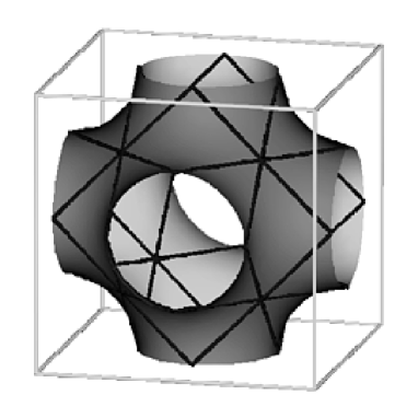
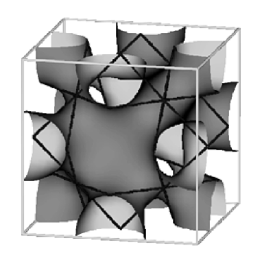
P	C(P)
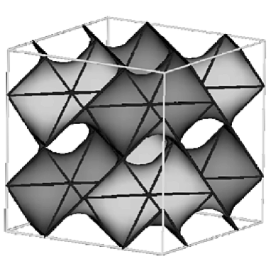
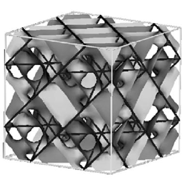
D	C(D)

FIG. 1.: Different TPMS with the same space group and the same system of straight lines. Spanning minimal surfaces are always balanced, thus they are characterized by a group-subgroup pair ${\cal G}-{\cal H}$. For P and C(P) this is $Im\bar{3}m$ (No. 229) - $Pm\bar{3}m$ (No. 221) and for D and C(D) this is $Pn\bar{3}m$ (No. 224) - $Fd\bar{3}m$ (No. 227).

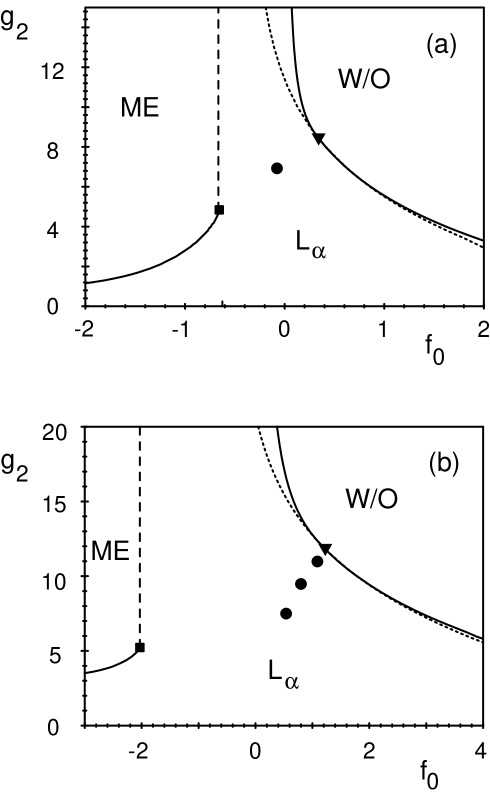
FIG. 2.: Phase diagram for the Ginzburg-Landau model (7), (8) for (a) $g_{0}=-3.0$ and (b) $g_{0}=-4.5$. Stable phases are the microemulsion ME, the lamellar phase $L_{\alpha}$ and the water and oil excess phases W and O. First and second order transitions are drawn by solid and dashed lines, respectively. Tricritical points are marked by squares and unbinding points by triangles. The dotted line in the $L_{\alpha}$ stability region is the $\sigma=0$-line. Metastable cubic phases are calculated at the points marked by full circles.

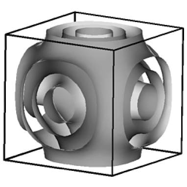
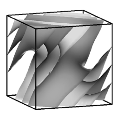
P	D
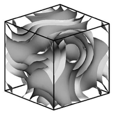
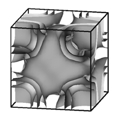
G	I-WP

FIG. 3.: Visualization of single and double structures for P, D, G and I-WP by their interfaces. The interfaces of the single structures appear as middle surfaces to the bilayers of the double structures. For the single D only one eighth of the unit cell is shown.

FIG. 4.: Distribution of mean curvature $H$ (top) and Gaussian curvature $K$ (bottom) in a conventional unit cell, plotted as histograms for the structures P, D, G and I-WP, for which Weierstrass representations are known. Radii of curvature are measured in units of the lattice constant. For $K$, we also plot as solid lines the distributions calculated from the Weierstrass representations. Due to the existence of Bonnet transformations between P, D and G, they have the same shape but different scales in these cases. The parameters in the Ginzburg-Landau model are the same as in Fig. 2a and the $K$-distributions are normalized to $\int dKp(K)=1$. For these “simple” structures, about 30 Fourier modes are sufficient.

FIG. 5.: Distribution of Gaussian curvature $K$ for single structures, for which no Weierstrass representations are known. The normalization is the same as in Fig. 4. These “complicated” structures have more pronounced modulation within the unit cell and larger lattice constants, therefore we use about 50 to 70 Fourier modes for the numerical minimization.

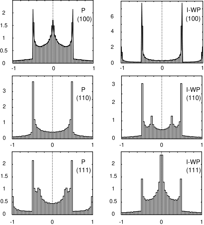
FIG. 6.: ${}^{2}H$-bandshapes for the structures P and I-WP and for the three high-symmetry directions $(100)$, $(110)$ and $(111)$. Results from the Weierstrass representations for the $(100)$-direction are drawn as solid lines.

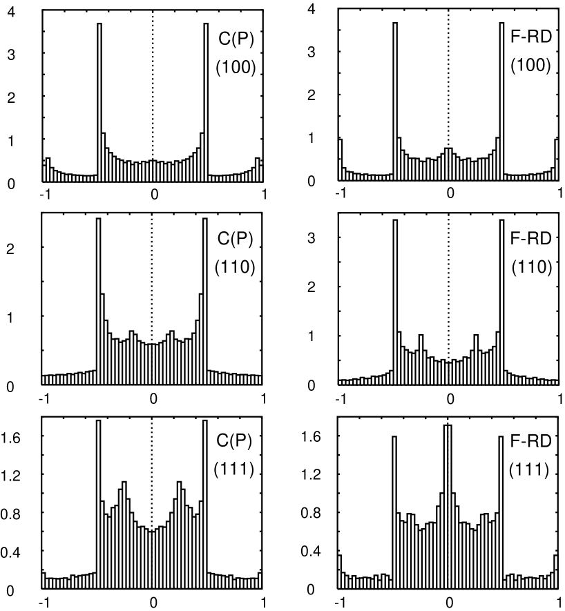
FIG. 7.: ${}^{2}H$-bandshapes for the structures C(P) and F-RD and for the three high-symmetry directions $(100)$, $(110)$ and $(111)$.

REFERENCES

- [1] Present address: Department of Materials and Interfaces, Weizmann Institute of Science, Rehovot 76100, Israel.
- [2] W. M. Gelbart, A. Ben-Shaul, and D. Roux, Micelles, Membranes, Microemulsions, and Monolayers (Springer, New York, 1994).
- [3] G. Gompper and M. Schick, in Self-assembling amphiphilic systems, Vol. 16 of Phase transitions and critical phenomena, edited by C. Domb and J. L. Lebowitz (Academic Press, London, 1994).
- [4] R. Lipowsky and E. Sackmann, Structure and Dynamics of Membranes, Vol. 1 of Handbook of biological physics (Elsevier, Amsterdam, 1995).
- [5] E. Dubois-Violette and B. Pansu, International Workshop on Geometry and Interfaces at Aussois, France, edited by E. Dubois-Violette and B. Pansu, special issue of J. Phys. (Paris) Colloq. C7 (1990).
- [6] D. M. Anderson and H. Wennerström, J. Phys. Chem. 94, 8683 (1990).
- [7] K. Fontell, Colloid Polym. Sci. 268, 264 (1990).
- [8] V. Luzzati et al., J. Mol. Biol. 229, 540 (1993).
- [9] J. M. Seddon and R. H. Templer, in Structure and dynamics of membranes - from cells to vesicles, Vol. 1A of Handbook of biological physics, edited by R. Lipowsky and E. Sackmann (Elsevier, Amsterdam, 1995), pp. 97–160.
- [10] D. M. Anderson, S. M. Gruner, and S. Leibler, Proc. Natl Acad. Sci. USA 85, 5364 (1988).
- [11] Z.-G. Wang and S. A. Safran, Europhys. Lett. 11, 425 (1990).
- [12] S. Hyde et al., The language of shape (Elsevier, Amsterdam, 1997).
- [13] T. Landh, FEBS Letters 369, 13 (1995).
- [14] G. S. Attard, J. C. Glyde, and C. G. Göltner, Nature 378, 366 (1995).
- [15] E. Pebay-Peyroula, G. Rummel, J. P. Rosenbusch, and E. M. Landau, Science 277, 1676 (1997).
- [16] W. Góźdź and R. Hołyst, Phys. Rev. E 54, 1 (1996).
- [17] G. Gompper and M. Schick, Phys. Rev. Lett. 65, 1116 (1990).
- [18] G. Gompper and S. Zschocke, Phys. Rev. A 46, 4836 (1992).
- [19] Q. Sheng, Ph.D. thesis, Cornell University, 1994.
- [20] Q. Sheng and V. Elser, Phys. Rev. B 49, 9977 (1994).
- [21] H. G. von Schnering and R. Nesper, Z. Phys. B 83, 407 (1991).
- [22] J. C. C. Nitsche, Lectures on minimal surfaces (Cambridge University Press, Cambridge, 1989).
- [23] U. Dierkes, S. Hildebrandt, A. Küster, and O. Wohlrab, Minimal Surfaces I and II, Vol. 295 of Grundlehren der mathematischen Wissenschaften (Springer, Berlin, 1992).
- [24] A. H. Schoen, Technical report, Washington, D.C. (unpublished).
- [25] H. Karcher, Manuscripta Math. 64, 291 (1989).
- [26] H. Karcher and K. Polthier, Phil. Trans. R. Soc. Lond. A 354, 2077 (1996).
- [27] W. Fischer and E. Koch, Phil. Trans. R. Soc. Lond. A 354, 2105 (1996).
- [28] W. Fischer and E. Koch, Z. Kristallogr. 179, 31 (1987).
- [29] R. L. E. Schwarzenberger, Bull. London Math. Soc. 16, 209 (1984).
- [30] M. Senechal, Crystalline symmetries - an informal mathematical introduction (Adam Hilger, Bristol, 1990).
- [31] R. Lifshitz, Rev. Mod. Phys. 69, 1181 (1997).
- [32] P. Ström and D. M. Anderson, Langmuir 8, 691 (1992).
- [33] J. O. Rädler, S. Radiman, A. de Vallera, and C. Toprakcioglu, Physica B 156, 398 (1989).
- [34] M. E. Cates et al., Europhys. Lett. 5, 733 (1988).
- [35] International tables for crystallography. Volume B: Reciprocal space, edited by U. Shmueli (Kluwer Academic Publishers, Dordrecht, 1996).
- [36] N. D. Mermin, Rev. Mod. Phys. 64, 3 (1992).
- [37] C. A. Lambert, L. H. Radzilowski, and E. L. Thomas, Phil. Trans. R. Soc. Lond. A 354, 2009 (1996).
- [38] I. S. Barnes, S. T. Hyde, and B. W. Ninham, J. Phys. (Paris) Colloq. 51, 7 (1990).
- [39] G. Gompper and M. Kraus, Phys. Rev. E 47, 4289 (1993).
- [40] P. B. Canham, J. Theor. Biol. 26, 61 (1970).
- [41] W. Helfrich, Z. Naturforsch. C 28, 693 (1973).
- [42] W. Góźdź and G. Gompper, unpublished.
- [43] R. Lipowsky and S. Leibler, Phys. Rev. Lett. 56, 2541 (1986).
- [44] S. Leibler and R. Lipowsky, Phys. Rev. Lett. 58, 1796 (1987).
- [45] M. Spivak, A comprehensive introduction to differential geometry I-IV (Publish or Perish, Houston, 1979).
- [46] D. M. Anderson, H. T. Davis, L. E. Scriven, and J. C. C. Nitsche, Adv. Chem. Phys. 77, 337 (1990).
- [47] G. Porod, Kolloid Z. u. Z. Polymere 124, 83 (1951).
- [48] L. Hsu, R. Kusner, and J. Sullivan, Exp. Math. 1, 191 (1992).
- [49] D. Anderson, H. Wennerström, and U. Olsson, J. Phys. Chem. 93, 4243 (1989).
- [50] S. T. Hyde, J. Phys. Chem. 93, 1458 (1989).
- [51] G. Gompper and M. Kraus, Phys. Rev. E 47, 4301 (1993).
- [52] R. Schneider, Convex bodies: the Brunn-Minkowski theory (Cambridge University Press, Cambridge, 1993).
- [53] R. Bruinsma, J. Phys. II France 2, 425 (1992).
- [54] P. M. Düsing, R. H. Templer, and J. M. Seddon, Langmuir 13, 351 (1997).
- [55] The opposite case of a positive saddle-splay modulus has been studied by C. N. Likos, K. R. Mecke, and H. Wagner, J. Chem. Phys. 102, 9350 (1995). In this case, a cutoff at small length scales is required to keep the lattice constant of the cubic phases finite.
- [56] S. Radiman, C. Toprakcioglu, and A. R. Faruqi, J. Phys. France 51, 1501 (1990).
- [57] L. Golubović and T. C. Lubensky, Phys. Rev. B 39, 12110 (1989).
- [58] J. Seelig, Quarterly Reviews of Biophysics 10, 353 (1977).
- [59] D. M. Anderson, J. Phys. (Paris) Colloq. 51, 1 (1990).
- [60] W. Góźdź and R. Hołyst, J. Chem. Phys. 106, 1 (1997).
- [61] A. Fodgen and S. T. Hyde, Acta Cryst. A48, 442 (1992).
- [62] A. Fodgen and S. T. Hyde, Acta Cryst. A48, 575 (1992).
- [63] S. Lidin, S. T. Hyde, and B. W. Ninham, J. Phys. France 51, 801 (1990).
- [64] D. Cvijovic and J. Klinowski, Chem. Phys. Lett. 226, 93 (1994).