System of Dirac fermions with random-varying mass is studied in detail. We reformulate the system by transfer-matrix formalism. Eigenvalues and wave functions are obtained numerically for various configurations of random telegraphic mass $m(x)$. Localized and extended states are identified. For quasi-periodic $m(x)$, low-energy wave functions are also quasi-periodic and extended, though we are not imposing the periodic boundary condition on wave function. On increasing the randomness of the varying mass, states lose periodicity and most of them tend to localize. At the band center or the low-energy limit, there exist extended states which have more than one peak spatially separate with each other comparatively large distance. Numerical calculations of the density of states and ensemble averaged Green’s functions are explicitly given. They are in good agreement with analytical calculations by using the supersymmetric methods and exact form of the zero-energy wave functions.

1 Introduction

Random disordered system is one of the most important problem in condensed matter physics. In two or lower dimensions, it is expected that almost all states are localized by the existence of random potentials, and study of these random systems obviously requires non-perturbative methods. In most of cases there exists no controllable parameter for analytical calculation. However recently, exact results have been obtained in certain interesting disordered systems in low dimensions[1, 2, 3]. There almost all states are localized as expected from the general consideration, and extended states exist only at isolated points in physical parameter region. Mathematical tools like supersymmetric (SUSY) methods etc. play an important role in averaging quenched disorders.

The random hopping tight-binding (RHTB) model in one dimension is one of the most extensively studied model[3, 4, 5]. This model is related with a random spin chain, a doped spin ladder, etc. [4, 6]. By using SUSY methods, the density of states (DOS) and single-fermion Green’s functions were obtained for white-noise random hopping[3]. Recently, the case of non-locally correlated disorders was studied by extending SUSY methods[7, 8]. This generalization is practically important because in almost all real systems random disorders have nonlocal correlations.

In this paper we shall revisit the system of random-mass Dirac fermion, which describes low-energy excitations near the band center of the RHTB model. However our approach in this paper is somewhat different from those given so far, and we hope that our study and previous works are complementary with each other. In most of studies, average over quenched disorder is taken in order to obtain physical quantities. In this paper however, we shall first study quantum mechanical states in various fixed random disorder backgrounds. To end this, we use the transfer matrix (TM) formalism. The TM formalism was used to calculate the transmission and reflection coefficients of current incident to a one-dimensional disordered system having a certain momentum[9]. In this paper, we shall extend the TM formalism and apply it to bound states and/or localized states to find their energy eigenvalues and wave functions. On controlling randomness, we can see how states tend to localize and what kind of states remain extended and contribute to long-distance correlations. To this end, results of our previous study on non-locally correlated disorder case is quite useful. After this observation, we shall take an ensemble average with respect to random variables and calculate the DOS and Green’s functions. We show that numerical calculations are in good agreement with analytical results in Refs.[7, 3] which were obtained by the SUSY methods and explicit form of zero-energy wave functions. This verifies that the SUSY methods give correct results.

This paper is organized as follows. In Sect.2, field equations of random-mass Dirac fermion is given. In Sect.3, we shall consider field equations in telegraphic configurations of random mass and reformulate the system by introducing the TM formalism. In the TM formalism, the eigenvalue problem of the Dirac field reduces to a simple matrix equation. Wave functions are also easily obtained by numerical calculation in the TM formalism. Results of numerical calculation are given in Sect.4. We identify localized and extended states from the wave functions. In order to see this, our previous studies on non-locally correlated disorder are quite useful. Especially it is shown that the DOS obtained by the numerical methods is in good agreement with the previous analytical calculation.We also obtain the ensemble averaged Green’s functions at vanishing energy or for nodeless states and compare them with analytic expression in Ref.[3]. They are in good agreement though the exact zero-energy wave functions used in the analytic calculation are not always normalizable contrary to those in the numerical calculation. Section 5 is devoted for discussion. We shall discuss relationship between the localization length and the number of states with energy below $E$. Some application of the results for spin chains is also discussed.

2 Field equations

We shall consider a Dirac fermion in one spatial dimension with coordinate-dependent mass whose Hamiltonian is given by,

$${\cal H} = \int dx\psi^{\dagger}h\psi,$$ (2.1)

$$h = -i\sigma^{z}\partial_{x}+m(x)\sigma^{y},$$ (2.2)

where $\vec{\sigma}$ are the Pauli matrices. Defining each component of $\psi$ as $\psi=(u,v)$, we can write the Dirac equation as,

$$\left(\ \frac{d}{dx}\ +\ m(x)\ \right)\ u(x) = Ev(x),$$

$$\left(\ -\frac{d}{dx}\ +\ m(x)\ \right)\ v(x) = Eu(x).$$ (2.3)

From Eqs.(2.3), we obtain Schr$\ddot{\mbox{o}}$dinger equations,

$$\left(\ -\frac{d^{2}}{dx^{2}}\ -m^{\prime}(x)+m^{2}(x)\ \right)\ u(x) = E^{2}u(x),$$

$$\left(\ -\frac{d^{2}}{dx^{2}}\ +m^{\prime}(x)+m^{2}(x)\ \right)\ v(x) = E^{2}v(x),$$ (2.4)

where prime denotes derivative with respect to the space coordinate. The exact solutions to (2.3) for $E=0$ are easily found though they are not always normalizable,

$$u,v\propto\exp\left[\ \pm\int dx\ m(x)\ \right].$$ (2.5)

However, solutions for positive eigen-values of $E$ cannot be represented in a simple form as in (2.5).

On the other hand, when $m(x)$ has a soliton-like configuration, such as

$$m(x)=\bar{m}\tanh(\lambda\bar{m}x),$$ (2.6)

the lowest-energy eigenstate for $\lambda=1$ is a “bound” state and explicitly given by

$$u(x)=\frac{1}{\cosh^{2}\bar{m}x},\;\;\;v(x)=0.$$ (2.7)

We call the configuration (2.6) for $\lambda>0$ anti-soliton and that for $\lambda<0$ soliton. It is one of our conjecture that localized states in the random potential, $V_{r}(x)=\pm m^{\prime}(x)+m^{2}(x)$, are essentially given by linear combinations of the above bound states in soliton and anti-soliton configuration of $m(x)$. To see this, we approximate the random potential to be a repetition of anti-soliton-soliton like configurations (2.6) and further, deform it to a series of the step functions by taking the limit $\lambda\to\infty$;

$$m(x)=\sum_{i}\bar{m}(\theta(x-\alpha_{i})-1)+\sum_{j}\bar{m}(\theta(-x+\beta_{j})-1)+m_{0},$$ (2.8)

where $\alpha_{i}$ and $\beta_{j}$ are positions of solitons and anti-solitons, respectively (see Fig.1). In the subsequent sections, we shall solve the Schr$\ddot{\mbox{o}}$dinger equations in the random background (2.8).

\begin{picture}(15.0,5.0)\centerline{\hbox{ \epsfbox{example.eps} }} \end{picture}

Figure 1: An example of configurations of solitons and anti-solitons, or “rectangular barriers” (Eq.(2.8)).

3 Eigenfunctions

For nonzero $E$, solutions of the Dirac equation (2.3) cannot be expressed in a general form as in (2.5). However, if we take the limit $\lambda\to\infty$, $m(x)$ takes alternatively two values $m_{0}+\bar{m}$ and $m_{0}-\bar{m}$ on intervals whose lengths are positive random variables. This drastically simplifies the problem and we can calculate the energy eigenfunctions for nonzero $E$ systematically using transfer matrices. In the first half of this section, solution in the background $m(x)$ with one step function is considered as a special case, and in the second half, it is shown that by connecting so obtained solutions, one can obtain solutions for arbitrary patterns of anti-soliton-soliton pairs.

3.1 Step-functional background

We study the Dirac equation (2.3) with a mass configuration which has a “domain wall” at $x=0$,

$$m(x)=\bar{m}(2\theta(-x)-1)+m_{0},$$ (3.1)

where $\theta(x)$ is the Heaviside function,

$$\theta(x)=\left\{\begin{array}[]{ccc}0&&(x<0)\\ 1&&(0<x)\end{array}\right.,$$ (3.2)

and it is assumed that

$$\bar{m}>m_{0}>0.$$

Substituting (3.1) into (2.4), we obtain a Schr$\ddot{\mbox{o}}$dinger equation with a potential which is a combination of the delta function and the step function,

$$V(x)=\mp m^{\prime}(x)+m^{2}(x)=\pm 2\bar{m}\delta(x)+4m_{0}\bar{m}\theta(-x)+(\bar{m}-m_{0})^{2}.$$ (3.3)

For such a field equation with a delta-function-type potential, the continuity of the wave function $u(x)$ leads automatically to the conditions on its derivative $u^{\prime}(x)$. For example, if we rewrite the Schr$\ddot{\mbox{o}}$dinger equation as

$$\left(-\frac{d^{2}}{dx^{2}}+2\bar{m}\ \delta(x)+4m_{0}\bar{m}\ \theta(-x)\right)\ u(x)=(E^{2}-(\bar{m}-m_{0})^{2})\ u(x)$$ (3.4)

and integrate Eq.(3.4) with respect to $x$ in the range $-\epsilon\leq x\leq\epsilon$, we have

$$-u^{\prime}(0+\epsilon)+u^{\prime}(0-\epsilon)+2\bar{m}\ u(0)+4m_{0}\bar{m}\int^{0}_{x}dx\ u(x)=(E^{2}-(\bar{m}-m_{0})^{2})\int^{\epsilon}_{-\epsilon}dx\ u(x).$$ (3.5)

However, the integrations in Eq.(3.5) vanish in the limit $\epsilon\to 0$ due to the continuity of $u(x)$. A similar argument applies to $v(x)$ and we have conditions,

$$u^{\prime}(0+0)-u^{\prime}(0-0) = 2\bar{m}u(0),$$

$$v^{\prime}(0+0)-v^{\prime}(0-0) = -2\bar{m}v(0).$$ (3.6)

We look for solutions under these conditions.

Let the energy eigenvalue $E$ satisfy

$$\bar{m}-m_{0}>E>0,$$ (3.7)

then $u(x)$ takes the form

$$u(x) = \left\{\begin{array}[]{ccc}A\ e^{\kappa_{1}x}+B\ e^{-\kappa_{1}x}&&(x<0),\\ C\ e^{\kappa_{2}x}+D\ e^{-\kappa_{2}x}&&(0<x),\end{array}\right.$$ (3.10)

$$\kappa_{1} = \sqrt{(\bar{m}+m_{0})^{2}-E^{2}},$$ (3.11)

$$\kappa_{2} = \sqrt{(\bar{m}-m_{0})^{2}-E^{2}}.$$ (3.12)

From the continuity of $u(x)$,

$$A+B=C+D$$ (3.13)

and Eq.(3.6) gives

$$\kappa_{2}(C-D)-\kappa_{1}(A-B)=2\bar{m}(A+B).$$ (3.14)

Hence,

$$u(x)=Ae^{\kappa_{1}x}+Be^{-\kappa_{1}x},\hskip 11.38109pt{\rm for}\hskip 11.38109ptx<0\\$$ (3.15)

and for $x>0$,

$$u(x) = \left[\ \frac{2\bar{m}-\kappa_{1}+\kappa_{2}}{2\kappa_{2}}A+\frac{2\bar{m}+\kappa_{1}+\kappa_{2}}{\kappa_{2}}B\ \right]\ e^{\kappa_{2}x}$$ (3.16)

$$+\left[\ \frac{-2\bar{m}+\kappa_{1}+\kappa_{2}}{2\kappa_{2}}A+\frac{-2\bar{m}-\kappa_{1}+\kappa_{2}}{\kappa_{2}}B\ \right]\ e^{-\kappa_{2}x}.$$

If we let $m_{0}=0$, $\kappa_{1}=\kappa_{2}$ and Eq.(3.16) simplifies to

$$u(x)=\left\{\begin{array}[]{cc}A\ e^{\kappa x}+B\ e^{-\kappa x},&\hskip 22.76219pt(x<0)\\ &\\ \displaystyle{\left[\ \frac{\bar{m}}{\kappa}A+\frac{\bar{m}+\kappa}{\kappa}B\ \right]\ e^{\kappa x}+\left[\ \frac{-\bar{m}+\kappa}{\kappa}A-\frac{\bar{m}}{\kappa}B\ \right]e^{-\kappa x}}.&\hskip 22.76219pt(0<x)\end{array}\right.$$ (3.17)

Values of $A,\ B$ and $E$ are determined by boundary conditions, e.g., $u(-L/2)=u(L/2)=0$ for a given system size $L$.

Our assumption that $u(x)$ remains continuous in the limit $\lambda\to\infty$ is justified as follows. The Schr$\ddot{\mbox{o}}$dinger equation with the potential

$$V(x) = \pm m^{\prime}(x)+m^{2}(x),$$

$$m(x) = \bar{m}\tanh(\lambda\bar{m}x)$$ (3.18)

is transformed to hyper-geometric differential equation by the change of variables,

$$z=\frac{1}{1+e^{-2\lambda\bar{m}x}},$$ (3.19)

and solved exactly. If we let $\lambda$ tend to infinity, the solution coincides with (3.16).

3.2 Transfer-matrix formalism

In this subsection we restrict $m_{0}$ to be zero. Since the wave function $u(x)$ is expressed everywhere as

$$u(x)=A\ e^{\kappa x}+B\ e^{-\kappa x},$$ (3.20)

we represent the eigenfunction in terms of coefficients $A$ and $B$ in what follows. By using matrix representation and from (3.16), the conditions (3.6) gives the following relation between the coefficients $A$ and $B$,

$$\left(\begin{array}[]{c}A(x>0)\\ B(x>0)\end{array}\right) = T\left(\begin{array}[]{c}A(x<0)\\ B(x<0)\end{array}\right),$$ (3.25)

$$T = \left(\begin{array}[]{cc}\displaystyle{1+\frac{\bar{m}}{\kappa}}&\displaystyle{\frac{\bar{m}}{\kappa}}\\ &\\ \displaystyle{-\frac{\bar{m}}{\kappa}}&\displaystyle{1-\frac{\bar{m}}{\kappa}}\end{array}\right).$$ (3.29)

For soliton instead of anti-soliton, one should replace $\bar{m}$ with $(-\bar{m})$ in Eq.(3.29) and one obtains

$$\left(\begin{array}[]{c}A(x>0)\\ B(x>0)\end{array}\right)=T^{-1}\left(\begin{array}[]{c}A(x<0)\\ B(x<0)\end{array}\right).$$ (3.30)

Let us define

$$R(\kappa,a) \equiv \left(\begin{array}[]{cc}e^{\kappa a}&0\\ 0&e^{-\kappa a}\end{array}\right),$$ (3.33)

$$\phi \equiv \frac{\bar{m}}{\kappa},$$ (3.34)

and TM for the configuration of an anti-soliton and a soliton is given as

$$R(b)T^{-1}R(a)T$$ (3.37)

$$= \left(\begin{array}[]{cc}(1-\phi^{2})e^{\kappa(a+b)}+\phi^{2}e^{\kappa(b-a)}&\phi(1-\phi)\left[e^{\kappa(a+b)}-e^{\kappa(b-a)}\right]\\ \phi(1+\phi)\left[e^{\kappa(a-b)}-e^{-\kappa(a+b)}\right]&(1-\phi^{2})e^{-\kappa(a+b)}+\phi^{2}e^{\kappa(a-b)}\end{array}\right)$$

$$= R(b)\left(\begin{array}[]{cc}e^{\kappa a}-2\phi^{2}\sinh\kappa a&2\phi(1-\phi)\sinh\kappa a\\ 2\phi(1+\phi)\sinh\kappa a&e^{-\kappa a}+2\phi^{2}\sinh\kappa a\end{array}\right)$$ (3.40)

$$\equiv T(a,b),$$ (3.41)

where $a$ is the distance between the soliton and anti-soliton. We impose boundary condition on the wave function such that the wave function vanishes as $|x|$ tends to large. This means that the solution, which is proportional to $e^{\kappa x}$ for $x\to-\infty$, does not have the factor of $e^{\kappa x}$ for $x\to\infty$. Hence $\kappa$ needs to satisfy

$$\left(\begin{array}[]{cc}1&0\end{array}\right)T(a,b)\left(\begin{array}[]{c}1\\ 0\end{array}\right)=e^{\kappa b}(e^{\kappa a}-2\phi^{2}\sinh\kappa a)=0.$$ (3.42)

Since $e^{\kappa b}\neq 0$, this means

$$\frac{\kappa^{2}}{\bar{m}^{2}}=1-e^{-2\kappa a}.$$ (3.43)

The energy eigenvalue $E$ tends to vanish in the limit $\kappa\to\bar{m}$, $a\to\infty$, as expected. If there are two pairs of anti-soliton and soliton, the boundary condition leads to

$$\left(\begin{array}[]{cc}1&0\end{array}\right)T(c,d)T(a,b)\left(\begin{array}[]{c}1\\ 0\end{array}\right)=0,$$ (3.44)

or

$$0 = e^{\kappa(a+b+c)}+2\phi^{2}[\ \sinh\kappa a\ \sinh\kappa c\ e^{-\kappa b}-e^{\kappa(b+c)}\sinh\kappa a-e^{\kappa(a+b)}\sinh\kappa c\ ]$$ (3.45)

$$+8\phi^{4}\sinh\kappa a\sinh\kappa b\sinh\kappa c.$$

The above argument can be generalized to an arbitrary numbers of anti-soliton-soliton pairs readily and we have the following eigenvalue equation,

$$\left(\begin{array}[]{cc}1&0\end{array}\right)T(e,f)\cdots T(c,d)T(a,b)\left(\begin{array}[]{c}1\\ 0\end{array}\right)=0.$$ (3.46)

It is easily seen that variables $\kappa$, $\bar{m}$ and distances between solitons $a,b,c,\cdots$ appear always in the combinations $\bar{m}/\kappa$, $\kappa a$,etc. Hence the eigenvalue equation (3.46) is invariant under a transformation

$$E\to\alpha E,\hskip 11.38109pt\bar{m}\to\alpha\bar{m},\hskip 11.38109pta\to a/\alpha$$ (3.47)

with an arbitrary positive constant $\alpha$. This property becomes important when we discuss relation between the localization length and the energy dispersion as we shall see in later sections. We are not able to solve (3.46) analytically for arbitrary configuration of pairs of solitons. However it is not so difficult to solve (3.46) numerically. We can also easily obtain eigenfunctions after having eigenvalues by using the TM. In subsequent sections, we shall give solutions to Eq.(3.46) obtained numerically for various multi-soliton configurations $m(x)$. Then we shall compare the results with the analytical calculation by the SUSY methods in our previous paper[7]. It is straightforward to extend the above formalism for nonvanishing $m_{0}$. Numerical solutions will be given also for $m_{0}\neq 0$.

4 Results of numerical calculation

4.1 Overview

We solved (3.46) numerically in various multi-soliton backgrounds, and obtained explicit form of corresponding eigenfunctions. We are interested in the relationship between randomness and localization of eigenfunctions. Then we compare wave functions of the eigenstates in quasi-periodical backgrounds and random backgrounds.

1. Quasi-Periodic Background

   First, we consider a quasi-periodic background in a system of finite size $L$, with almost equal distances between each successive soliton and anti-soliton. Eigenfunctions obtained by numerical calculations show twofold oscillations, i.e., rapid oscillations occurring at positions of soliton and anti-soliton, and slowly oscillating envelope (see the graphs at the top of Fig.2). The peaks of rapid oscillation can be considered essentially the same as the bound state (2.7) in a single soliton background, because in a background of sufficiently separated solitons, eigenfunctions can be approximated by a linear combination of bound states located at solitons and anti-solitons.

   The envelope of eigenfunctions is reminiscent of sine curves and the nodes of eigenfunctions coincide with those of corresponding sine curves. Frequencies of the envelopes are larger for higher energy eigenvalue and this supports “one-dimensional node counting theorem”[2], which states that the number of nodes of eigenfunction increases with eigenenergy.

   In quasi-periodic background, all eigenstates extend over the whole system and there are no localized eigenstates. This is reminiscent of Bloch’s theorem although we do not impose the periodic boundary condition on the wave functions.

   \begin{picture}(15.0,15.0)\centerline{\hbox{ \epsfbox{quasiperiod1.eps} }} \end{picture}

   

   Figure 2: The shapes of $u(x)$ in rectangular barriers distributed according to gaussian distribution with the average lengths $\langle l\rangle=2$ and $\bar{m}=1$. In this figure $n$ denotes the state of $n$-th energy from the lowest and $m_{0}$ is set to zero. The graphs at the top are those in a periodic potential, where the standard deviation $\sigma=0$. Here $\sigma$ increases from zero at the top to $0.6$ at the bottom by $0.2$. Eigenfunctions $v(x)$ have similar behavours to $u(x)$.

2. Randomly Distributed Barriers: $m_{0}=0$

   We now vary the distances between soliton and anti-soliton according to the gaussian distribution, i.e., lengths of rectangular barriers $l$ are subject to the gaussian distribution,

   $$P_{{\rm G}}(l)=\frac{1}{\sqrt{2\pi}\sigma}\exp\{-(l-\mu)^{2}/2\sigma^{2}\}.$$ (4.1)

   $m_{0}$ is set to zero here. In this case, the periodicity of eigenfunction is lost as randomness or $\sigma$ in Eq.(4.1) increases and the envelope has a large peak. This means all the states tend to “localize” (see Fig.2). The state of the lowest energy $E\simeq 0$ extends over the whole system as it can be expected from the formula (2.5). Low-energy states are still extended even at $\sigma=0.4$.

   \begin{picture}(15.0,10.0)\centerline{\hbox{ \epsfbox{exp1.eps} }} \end{picture}

   

   Figure 3: The shapes of $u(x)$ in rectangular barriers whose lengths $l$ are distributed according to exponential distribution with $\tilde{\lambda}=0.25$ (Eq.(4.3)). In this figure $n$ denotes the state of $n$-th energy from the lowest. $\bar{m}$ and $m_{0}$ are set as $m_{0}=0$ and $\bar{m}=1$.

   The degree of randomness is controlled by the variance of gaussian distribution $\sigma$. For larger $\sigma$, shapes of wavefunctions become sharper and the states become more localized. We took a close look at various numerical results and found that some of the states have more than one dominant peak in two or three intervals between nodes and others have only single “large” peak and are localized in an interval between adjacent nodes. Let $N(E)$ denotes the number of states from the lowest to the energy $E$ per unit length. Since the width of the interval is approximately proportional to $1/N(E)$, we are led to a conjecture that the localization length $\xi(E)$ satisfies

   $$\xi(E)=\frac{A}{N(E)}.$$ (4.2)

   The proportional coefficient $A$ seems to depend on the distribution of the length of rectangular barriers $l$, $\bar{m}$ and $L$, but not on $E$.

   In Fig.3, we show eigenfunctions in random rectangular barriers whose lengths $l$ are distributed according to the following exponential distribution instead of (4.1),

   $$P_{{\rm E}}(l)=\frac{1}{2\tilde{\lambda}}\exp\left[-\frac{l}{2\tilde{\lambda}}\right].$$ (4.3)

   From these results, we can see that the localization around one peak is enhanced in higher-energy states. We also verified that as $\tilde{\lambda}$ increases extended states are hindered, just as in the gaussian distribution.

3. For $m_{0}\neq 0$

   In the above we dealt only with the case of vanishing $m_{0}$. Here, we take $m_{0}\neq 0$. For quasi-periodic backgrounds, states are still periodic and extended. “Bloch’s theorem” is valid as in the case of $m_{0}=0$. If we vary the length of barrier $l$ randomly, states are more localized than in the case of vanishing $m_{0}$ (see Fig.4). Thus we conclude that nonzero $m_{0}$ is not necessary for localization, but at least it seems to enhance the localization.

   \begin{picture}(15.0,10.0)\centerline{\hbox{ \epsfbox{exp2.eps} }} \end{picture}

   

   Figure 4: The shapes of $u(x)$ in rectangular barriers whose lengths $l$ are distributed according to exponential distribution with $\tilde{\lambda}=0.25$ (Eq.(4.3)). In this figure $n$ denotes the state of $n$-th energy from the lowest. The parameters $\bar{m}$ and $m_{0}$ are set as $m_{0}=0.3$ and $\bar{m}=1$.

4.2 Comparison with the analytical results: Density of states

Although Dirac fermion systems with non-locally correlated mass $m(x)$ have seldom been studied, the case of exponentially distributed $m(x)$ was studied recently by Comtet et.al.[2] via stochastic method and more systematically by Ichinose and Kimura [7] via SUSY methods. Analytical expression of the DOS was obtained there. We calculate the DOS numerically by using the TM method and compare the result with analytical expression.

For locally distributed $m(x)$, the density of states with energy $E$, $\rho(E)={dN(E)\over dE}$, is given by

$$\rho(E)\propto\frac{1}{|\ln E|^{3}},$$ (4.4)

as $E$ tends to small. For non-locally correlated random mass $m(x)$[7],

$$\rho_{\tilde{\lambda}}(E) = \hskip 11.38109pt\frac{1}{2\frac{E}{4g}|\ln\frac{E}{4g}|^{3}}$$ (4.5)

$$-4g\tilde{\lambda}\frac{3}{2\frac{E}{4g}|\ln\frac{E}{4g}|^{4}}$$

$$+16g^{2}\tilde{\lambda}^{2}\left(\frac{13}{30\frac{E}{4g}|\ln\frac{E}{4g}|^{3}}-\frac{1}{2\frac{E}{4g}|\ln\frac{E}{4g}|^{4}}+\frac{1}{\frac{E}{4g}|\ln\frac{E}{4g}|^{5}}\right)$$

$$-(4g)^{3}\tilde{\lambda}^{3}\frac{1}{210\frac{E}{4g}|\ln\frac{E}{4g}|^{3}}+{\cal O}(\tilde{\lambda}^{4}),$$

where $g$ and $\tilde{\lambda}$ are defined as

$$[\ m(x)\ m(y)\ ]_{{\rm ens}}=\frac{g}{\tilde{\lambda}}\exp\ (-|x-y|/\tilde{\lambda}).$$ (4.6)

Parameter $\tilde{\lambda}$ is the correlation length of the disorder. As $\tilde{\lambda}\rightarrow 0$, $m(x)$ and $m(y)$ for $x\neq y$ become uncorrelated, the white-noise limit.

Distribution corresponding to (4.6) can be realized by rectangular barriers whose height is

$$\bar{m}=\sqrt{\frac{g}{\tilde{\lambda}}},$$ (4.7)

and width between solitons, $l$, is distributed as[2]

$$P(l)=\frac{1}{2\tilde{\lambda}}\exp\left[-\frac{l}{2\tilde{\lambda}}\right].$$ (4.8)

The result of numerical calculation of 300 pairs of a soliton and anti-soliton is shown in Fig.5. We obtained the number of states $N_{num}(E)$ by numerical calculation, and we define $\rho_{num}$ as the averaged density of states around the energy level $E$ as

$$\rho_{num}(E)=\frac{N_{num}(E+\frac{\Delta E}{2})-N_{num}(E-\frac{\Delta E}{2})}{\Delta E}.$$ (4.9)

In order to compare the numerical result of the density of states with energy $E$ with the analytical expression $\rho_{\tilde{\lambda}}(E)$ in (4.5), we see the ratio $r(E)=\frac{\rho_{\tilde{\lambda}}(E)}{\rho_{num}(E)}$. If the energy dependence of these density of states coincides, this ratio $r(E)$ should be constant. In Fig.5. $r(E)$ is shown. From this, we can conclude that the energy spectrum of the states obtained by the numerical calculation is in good agreement with the analytical result (4.5). Especially, the higher-order expression of $\rho_{\tilde{\lambda}}(E)$ in (4.5) gives the better agreement. This result also indicates that 300 pairs of a soliton and anti-soliton is large enough for the investigation of the system in the low-energy region.

\begin{picture}(15.0,10.0)\centerline{\hbox{ \epsfbox{ratio.eps} }} \end{picture}

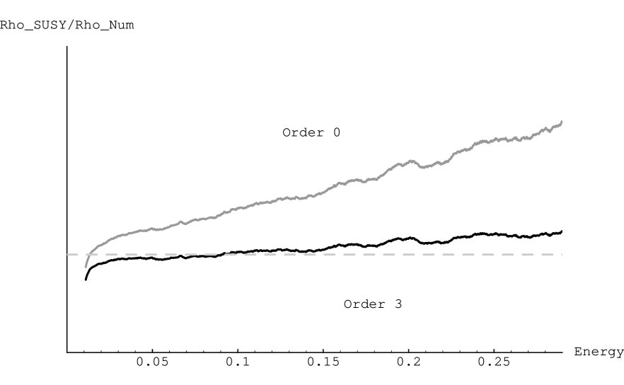
Figure 5: Energy spectrum of fermion: A comparison between the result of numerical calculation and $\rho_{\tilde{\lambda}}(E)$ of the zero-th order and up to the third order in $\tilde{\lambda}$, Eq.(4.5). Here we set $\tilde{\lambda}=1/6$, $g=1$, $\Delta E=0.02$ and numerical result is averaged over 4000 trials. The ratio $r(E)$ is shown in this figure. If the numerical calculation agrees with $\rho_{\tilde{\lambda}}(E)$ which is obtained by SUSY methods, the ratio should be constant. The dashed line is expected exact result.

4.3 Green’s functions at vanishing energy

In this section, we show numerical result of the ensemble averaged Green’s functions at vanishing energy and compare them with analytical expression in Refs.[3, 4].

The zero-energy wave functions are given by Eq.(2.5). It is not so difficult to calculate the ensemble-averaged correlation of them

$$W_{q}(x,L)=[|\psi^{\dagger}(x)\psi(0)|^{q}]_{{\rm ens}}$$ (4.10)

in the white-noise limit with the system size $L$[3, 4]. There the normalization of the wave functions plays an important role because only for specific $m(x)$ they are genuine normalizable functions. More explicitly, in solving the Dirac equation we imposed the boundary condition such that the wave function decays exponentially outside of the random potential. In the analytical calculation in [3, 4], such kind of boundary condition is not imposed on the wave function.

In general it is expected that the above correlation functions exhibit complex multi-fractal scaling as in the qunatum Hall state,

$$W_{q}(x,L)\sim L^{-d-\tau(q)}|x|^{-y(q)}.$$ (4.11)

For the present system, $W_{q}(x,L)$ is obtained as follows for $L\rightarrow\infty$,

$$W_{q}(x,L)\sim\frac{\tilde{W}(q^{2}x)}{L}$$ (4.12)

with

$$\tilde{W}(x)=\int^{\infty}_{0}dk\frac{k^{2}}{(1+k^{2})^{4}}e^{-xk^{2}}.$$ (4.13)

For large $x$

$$W_{q}(x,L)\sim 1/(x^{3/2}L)$$ (4.14)

and therefore it is expected that $\tau(q)=0$ and $y(q)=3/2$.

We numerically calculated the correlation functions $W_{q}(x,L)$ with various values of $q$. To this end, we focused on the states of nodeless wave function. The results are shown in Figs.6 and 7 for $q=0.5,\;1.0,\;1.2\;$ and $1.5$ as well as the analytical result Eqs.(4.12) and (4.13). It is obvious that the numerical calculations are in good agreement with the analytical calculations. Especially we can conclude that the critical exponent of the multi-fractal scaling is obtained as $y(q)=3/2$ independently of $q$. (It seems that $y(q)$ is smaller than $3/2$ for small $q$. But we expect that $y(q)$ with any $q$ approaches to $3/2$ for larger systems.)

We also study $L$ dependence of $W_{q}(x,L)$. The result is shown in Fig.8. According to this, it seems that $W_{q}(x,L)$ is not inversely proportional to $L$ and moreover $\tau(q)\neq 0$, contrary to the analytical calculation by Balents and Fisher[3]. We further calculated $W_{q}(x,L)$ for larger system size $L$ and smaller $g$, and obtained similar results. However it is still possible that the system size $L$ is not large enough in our numerical calculations. Therefore the above is not a definite conclusion and more systematic calculation is desired. (In the analytical calculation[3], $L$ is assumed to be large enough.)

We should again remark here that Eqs.(4.12) and (4.13) are obtained from (2.5) some of which are not normalizable. On the contrary, the wave functions in the numerical calculation are all normalizable. Then strictly speaking, one cannot expect coincidence of the analytical and numerical results.

\begin{picture}(15.0,15.0)\centerline{\hbox{ \epsfbox{fractal1.eps} }} \end{picture}

Figure 6: Multifractal behaviour of bound-state wavefunction (1) : The $x$ dependence of $W_{q}(x,L)$ based on numerical and analytical calculations is shown. Difference between two results is also shown. To calculate $W_{q}(x,L)$, we used the u-component of the doublet $\psi=(u,v)$, namely $W_{q}(x,L)_{num}=[|u(x+l)u(l)|]_{\rm ens}$. To obtain $W_{q}(x,L)_{num}$ numerically, we averaged $W_{q}$ over 2800 configurations of the random-varying mass. We also took an average with respect to $l$ in $[|u(x+l)u(l)|]_{\rm ens}$.

\begin{picture}(15.0,15.0)\centerline{\hbox{ \epsfbox{fractal2.eps} }} \end{picture}

Figure 7: Multifractal behaviour of bound-state wavefunction (2) : The method to obtain $W_{q}$ is the same as we mentioned in the caption of Fig.6. We can see that the inclination of $W_{q}$ with $q=1.2$ and $1.5$ is almost 3/2 in the region around $\log(x/L)\sim-1$. (We set $L$(the system size)$=40$, $\tilde{\lambda}=1/512$ and $g=1/2$ (almost white-noise case) in the numerical calculation, and we set $L=40$ and $g=1/2$ in the analytical calculation.)

\begin{picture}(12.0,15.0)\centerline{\hbox{ \epsfbox{fractal3.eps} }} \end{picture}

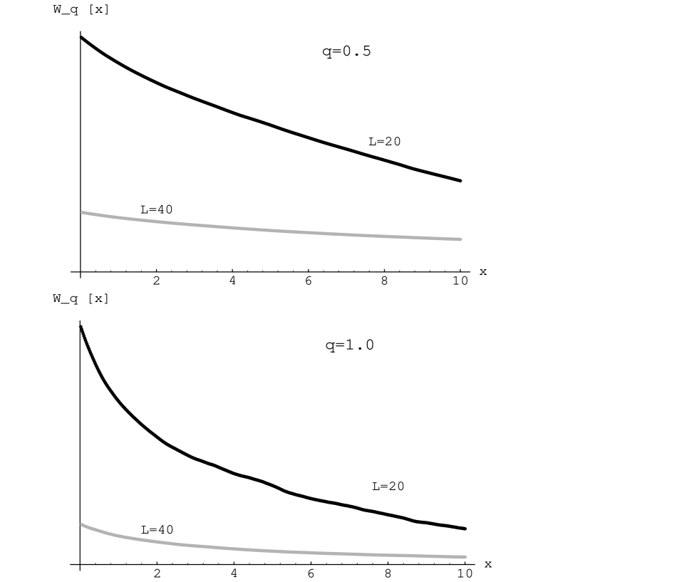
Figure 8: Multifractal behaviour of bound-state wavefunction (3) : $L$(the system size) dependence of $W_{q}(x,L)$ for $q=0.5$ and $1.0$ is shown. Here we set $\tilde{\lambda}=1/512$ and $g=1/2$, and $W_{q}$ is averaged over 1600 backgrounds of the random mass. To calculate $W_{q}\;$, we used only the u component, though we verfied that the v component behaves similarly.

5 Discussion

From the results of the DOS and the Green’s functions, we conclude that 300 pairs of a soliton and anti-soliton can be regarded as a good approximation for infinite-size system. Hence it is legitimate to discuss behaviors of the localized states based on properties of numerically obtained solutions.

Results obtained from the numerical calculations can be summarized as follows.

• For a quasi-periodic background, “Bloch’s theorem” is valid and all the states extend over the whole system, regardless of the value of $m_{0}$. The envelopes of wave functions are similar to sine curves.

• For $m_{0}=0$, on varying the length of rectangular barriers randomly, states begin to localize, within two or three intervals between nodes. Some of them, especially the lowest-energy states, has more than one peak which separate with each other rather long distance.

• For nonzero value of $m_{0}$, the states tend to localize in narrower intervals than in the case of $m_{0}=0$. Hence nonzero $m_{0}$ enhances, but is not necessary for the localization.

We conjectured that the averaged localization length $\xi(E_{n})$ for the $n$-th state from the lowest satisfies

$$\xi(E_{n})=\frac{A}{n},$$ (5.1)

since states in randomly distributed rectangular barriers are localized in two or three intervals between nodes and length of each interval $l(E_{N})$ is proportional to $1/N$. Here, $A$ in (5.1) depends on the distribution of lengths of rectangular barriers $l$, $\bar{m}$ and $L$, but not on energy $E$. One of supports for this conjecture is given by the exact result for locally correlated random mass $m(x)$, since the number of states below energy $E$ is given as

$$N(E)\propto\frac{1}{(\ln E)^{2}},$$ (5.2)

and localization length is given as

$$\xi(E)\propto(\ln E)^{2},$$ (5.3)

hence (5.1) is satisfied in this case. (Note that $N(E)$ and $n$ are related as $N=n/L$.) Very recently, we obtained the localization length of the ensemble-averaged one-particle Green’s functions by using the SUSY methods[8],

$$\xi(E)={1\over g\pi^{2}}\Big{(}|\ln{E\over 2g}|^{2}+4g\tilde{\lambda}|\ln{E\over 2g}|\Big{)}+O((g\tilde{\lambda})^{2}).$$ (5.4)

From this result and the DOS in Eq.(4.5), we can verify

$$\xi(E)N_{\tilde{\lambda}}(E)\propto 1+O((g\tilde{\lambda})^{2}).$$ (5.5)

We also performed numerical calculations with the TM method under Dirichlet boundary condition, which is $u(0)=u(L)=0$. However qualitatively features of the localization are the same. Another important insight into the Dirac fermion system with random mass $m(x)$ obtained by the present study is that the $n$-th state from the lowest is related to the lowest-energy state in system of size $1/N(=L/n)$, since a state localized inside an interval of length $1/N$ must be realized as the ground state of the system of length $1/N$.

The ensemble-averaged Green’s functions were also calculated. They are in good agreement with the analytical results. Especially, though each wave function exhibits rapid oscillations, the ensemble-averaged Green’s functions have smooth behaviour.

Finally let us comment on the spin systems closely related to the random-mass Dirac fermions. As discussed in Refs.[4, 6] low-energy excitations in doped spin-ladder or spin-Peierls systems are described by the random-mass Dirac fermions. Undoped cases of the above systems have an energy gap, and by doping there appear midgap states[11]. Results obtained in this paper suggest that properties of the midgap states strongly depend on the randomness of the doping, i.e., almost all midgap states are extended for quasi-periodic doping, whereas states tend to localize for random doping. In terms of spin-Peierls system (like the compound $\mbox{Cu}_{1-x}\mbox{Zn}_{x}\mbox{GeO}_{3}$ [12]), the localization length $\xi(E)$ is related with the correlation length of spins, since the existence or absence of our fermion is related to the up or down of the spins via Jordan-Wigner transformation[13]. Using our results one will be able to find that randomly doped spin-Peierls compounds have the short correlation length of spin. It is very interesting to see the above behavior by experiments in which the distribution of impurities is controled. We are now calculating Green’s functions in having more definte prediction for the above spin systems. The result will be reported in a future publication[8].

References

-
[1]
A. W. W. Ludwig, M. P. A. Fisher, R. Shanker and G. Grinstein,
Phys. Rev. B50 (1994) 7526.
C. Chamon, C. Mudry and X. G. Wen, Phys. Rev. Lett. 77 (1996) 4194.
I.I.Kogan, C. Mudry and A. M. Tsvelic, Phys. Rev. Lett. 77 (1996) 707.
D. S. Fisher, Phy. Rev. B 50 (1994) 3799; ibid., B51 (1995) 6411. - [2] A. Comtet, J. Desbois and C. Monthus, Ann. Phys. 239 (1994) 312.
- [3] L. Balents and M. P. A. Fisher, Phys. Rev. B56 (1997) 12970.
- [4] D. G. Shelton and A. M. Tsvelik, Phys. Rev. B57 (1998) 14242.
- [5] H. Mathur, Phys. Rev. B56 (1997) 15794.
- [6] A. O. Gogolin, A. A. Nersesyan, A. M. Tsvelik and Lu Yu, Nucl. Phys. B540 (1999) 705.
- [7] I. Ichinose and M. Kimura, cond-mat/9809323
- [8] I. Ichinose and M. Kimura, paper in preparation.
- [9] See e.g., P. Erds and R. C. Herndon, Adv. Phys. 31 (1982) 65.
- [10] A. J. Niemi and G. W. Semenoff, Phys. Rep. 135 (1986) 99.
- [11] M. Fabrizio and R. Mélin, Phys. Rev. Lett. 78 (1997) 3382.
- [12] M. Hase, I. Terasaki, Y. Sasago and K. Uchinokura, Phys. Rev. Lett. 71, (1993) 4059; J. Phys. Soc. Jpn. 65, (1996)1392.
- [13] T. D. Schltz, D. C. Mattis and E. H. Lieb, Rev. Mod. Phys. 36 (1964) 856.