Transverse-field Ising spin chain with inhomogeneous disorder

Abstract

We consider the critical and off-critical properties at the boundary of the random transverse-field Ising spin chain when the distribution of the couplings and/or transverse fields, at a distance $l$ from the surface, deviates from its uniform bulk value by terms of order $l^{-\kappa}$ with an amplitude $A$. Exact results are obtained using a correspondence between the surface magnetization of the model and the surviving probability of a random walk with time-dependent absorbing boundary conditions. For slow enough decay, $\kappa<1/2$, the inhomogeneity is relevant: Either the surface stays ordered at the bulk critical point or the average surface magnetization displays an essential singularity, depending on the sign of $A$. In the marginal situation, $\kappa=1/2$, the average surface magnetization decays as a power law with a continuously varying, $A$-dependent, critical exponent which is obtained analytically. The behavior of the critical and off-critical autocorrelation functions as well as the scaling form of the probability distributions for the surface magnetization and the first gaps are determined through a phenomenological scaling theory. In the Griffiths phase, the properties of the Griffiths-McCoy singularities are not affected by the inhomogeneity. The various results are checked using numerical methods based on a mapping to free fermions.

I Introduction and summary

Quantum systems with quenched disorder have received much attention recently, due to their unusual static and dynamical properties.[2] Many of these features can be observed in one-dimensional models for which several exact and conjectured results are available in the case of homogeneous disorder. Among these models we shall consider the random transverse-field Ising model (RTIM) defined by the Hamiltonian

$${\cal H}=-\frac{1}{2}\sum_{l}[J_{l}\sigma_{l}^{x}\sigma_{l+1}^{x}+h_{l}\sigma_{l}^{z}]\,,$$ (1)

where $\sigma_{l}^{x}$ and $\sigma_{l}^{z}$ are Pauli matrices at site $l$. The exchange couplings $J_{l}$ and the transverse fields $h_{l}$ are random variables with probability distributions $\pi_{l}(J)$ and $\rho_{l}(h)$, respectively, which are independent from each other but may depend on the position $l$. Note that in one dimension the couplings and the fields can be taken positive without loss of generality.

The homogeneously disordered model, with position-independent distributions $\pi_{l}(J)=\pi(J)$ and $\rho_{l}(h)=\rho(h)$, has received much attention, especially after Fisher has obtained new striking results about static critical properties and equal-time correlations, using a renormalization group method based on a decimation procedure.[3] Many of Fisher’s results have been later verified by numerical methods and some other analytical, scaling and numerical results have been obtained concerning the dynamical properties of the RTIM and the behavior of different probability distributions.[4, 5, 6, 7, 8, 9]

For the homogeneous model in (1) one defines the quantum control parameter as

$$\delta=[\ln h]_{\rm av}-[\ln J]_{\rm av}\,,$$ (2)

where $[\dots]_{\rm av}$ denotes an average over quenched disorder. The system is in the ferromagnetic (paramagnetic) phase when the couplings are in average stronger (weaker) than the transverse fields, thus for $\delta<0$ ($\delta>0$). The critical point corresponds to $\delta=0$.

In this paper we concentrate on the surface properties of the RTIM. The average surface magnetization, $[m_{s}(\delta)]_{\rm av}$, which can be studied using a mapping to a problem of surviving random walks (RW),[6] behaves as $[m_{s}(\delta)]_{\rm av}\sim-\delta$ close to the critical point, whereas the correlation length diverges as $[\xi]_{\rm av}\sim|\delta|^{2}$. Thus the corresponding critical exponents for the average quantities are:

$$\beta_{s}=1,\ \ \ \nu=2\,.$$ (3)

The scaling is strongly anisotropic at the critical point of the homogeneous RTIM: The time scale set by the relaxation time $\tau_{r}$ and the length scale $\xi$ are related through

$$\ln\tau_{r}\sim\xi^{1/2}\,.$$ (4)

As a consequence, the imaginary-time spin-spin autocorrelations are logarithmically slow at the critical point with

$$\left[G_{s}(\tau)\right]_{\rm av}\sim(\ln\tau)^{-1}\,,\ \ \ \delta=0\,,$$ (5)

for the surface spins. In the Griffiths phase, on the paramagnetic side of the critical point, the autocorrelations are still anomalous and decay like a power,

$$[G(\tau)]_{\rm av}\sim\tau^{-1/z(\delta)}\,,\ \ \ 0<\delta<\delta_{G}\,,$$ (6)

with a dynamical exponent $z(\delta)$ given by the positive root of the following equation:[7]

$$\left[\left({J\over h}\right)^{1/z}\right]_{\rm av}=1\,.$$ (7)

As shown recently,[8] all the singular quantities in the Griffiths phase (susceptibility, non-linear susceptibility, energy-density autocorrelations, etc) involve the dynamical exponent $z(\delta)$.

In many physical systems the disorder is not homogeneous. For example a free surface or an internal defect line may locally modify the distribution of the couplings and/or fields. Here we consider surface induced inhomogeneities which are characterized by a power-law variation in the probability distribution: $\pi_{l}(J)-\pi(J)\sim l^{-\kappa}$ and/or $\rho_{l}(h)-\rho(h)\sim l^{-\kappa}$, for $l\gg 1$, such that the local control parameter in (2) varies as

$$\delta(l)=\delta-Al^{-\kappa}\,.$$ (8)

Our choice for the functional form of the inhomogeneous disorder is analogous to the variation of the couplings in the so-called extended surface defect problem first introduced by Hilhorst and van Leeuwen (HvL) for the two-dimensional classical Ising model.[10] This type of inhomogeneity has been later studied for other models and different geometries. For a review see Ref.[11].

Informations about the critical properties of the RTIM with inhomogeneous surface disorder have been obtained by combining different approaches: The calculation of the surface magnetization can be mapped onto a problem of surviving RW’s, allowing us to deduce some exact results. The asymptotic behavior of the surface autocorrelation function and the form of the probability distribution for different quantities follow from a phenomenological scaling theory. They have been checked through large scale numerical calculations using the free fermion formulation of the RTIM.

TABLE I.: Summary of the surface critical properties of the inhomogeneous RTIM.

	$\ln\tau_{r}$	$P_{\epsilon}(\ln\epsilon_{1},L)$	$[m_{s}(\delta)]_{\rm av}$	$P_{m}(\ln m_{s},L)$	$\lim_{v\to 0}\widetilde{P}_{m}(v)$	$[G_{s}(\tau)]_{\rm av}$
$\kappa>1/2$	$\sim\xi^{1/2}$	${1\over L^{1/2}}\widetilde{P}_{\epsilon}\left[{\ln\epsilon_{1}\over L^{1/2}}\right]$	$\sim|\delta|$	${1\over L^{1/2}}\widetilde{P}_{m}\left[{\ln m_{s}\over L^{1/2}}\right]$	$\sim$const	$\sim(\ln\tau)^{-1}$
$\kappa=1/2$	$\sim\xi^{1/2}$	${1\over L^{1/2}}\widetilde{P}_{\epsilon}\left[{\ln\epsilon_{1}\over L^{1/2}}\right]$	$\sim|\delta|^{\beta_{s}(A)}$	${1\over L^{1/2}}\widetilde{P}_{m}\left[{\ln m_{s}\over L^{1/2}}\right]$	$\sim v^{1-\beta_{s}(A)}$	$\sim(\ln\tau)^{-\beta_{s}(A)}$
$\kappa<1/2$	$\sim\xi^{1-\kappa}$	${1\over L^{1-\kappa}}\widetilde{P}_{\epsilon}\left[{\ln\epsilon_{1}\over L^{1-\kappa}}\right]$	—	${1\over L^{1-\kappa}}\widetilde{P}_{m}\left[{\ln m_{s}\over L^{1-\kappa}}\right]$	—	—
$A>0$	—	—	$\sim|A|^{1\over 1-2\kappa},\,\delta=0$	—	$v^{-1}$	$\sim$ const
$A<0$	—	—	$\sim\exp[-{\rm const}\,|\delta|^{-(1-2\kappa)/\kappa}]$	—	0	$\sim\exp[-{\rm const}\,(\ln\tau)^{1-2\kappa\over 1-\kappa}]$

Our main results are summarized in Table I. The surface critical behavior of the inhomogeneous RTIM depends on the value of the decay exponent $\kappa$. For fast enough decay of the inhomogeneity, i.e., for $\kappa>1/2$, the surface critical properties of the model are the same as for the homogeneous RTIM. Specifically, the critical exponents keep the values given in Eq. (3) and relations (4) and (5) remain valid.

In the borderline case, $\kappa=1/2$, the effect of the inhomogeneity is marginal: the average surface magnetization has a distribution-dependent critical exponent, $\beta_{s}(A)$, which has been calculated analytically. This exponent governs also the logarithmic decay of the surface spin-spin autocorrelation function, like in Eq. (5) for the homogeneous case, but with a different value. The scaling relation between $\tau_{r}$ and $\xi$ keeps the form given in Eq. (4) for the homogeneous model. The same is true of the scaling behavior of the probability distributions for the energy gap $\epsilon$, and the surface magnetization $m_{s}$, at large system size $L$. The scaling function of the latter, however, has a different asymptotic behavior, which is connected to the different $\delta$-dependence of the average surface magnetization in the two cases.

For a slower decay, such that $\kappa<1/2$, the scaling relation in Eq. (4) is modified and leads to a new scaling form for the probability distributions of the energy gap and the suface magnetization. For enhanced surface couplings, $A>0$, the average surface magnetization remains finite at the bulk critical point. It vanishes as a power of $A$ when $A$ goes to zero from above. For weakened surface couplings, the average surface magnetization displays an essential singularity in $\delta$ instead of a power law, whereas the surface autocorrelation function has an enhanced power-law decay.

In the numerical calculations we used two types of distributions for the disorder. In the inhomogeneous binary distribution, the couplings take the values $\Lambda>1$ and $\Lambda^{-1}$ with probability $p_{l}=\frac{1}{2}(1+A_{b}l^{-\kappa})$ and $q_{l}=1-p_{l}$, respectively, while the transverse field remains constant:

$$\pi_{l}(J) = p_{l}\delta(J-\Lambda)+q_{l}\delta(J-\Lambda^{-1})\,,$$ (9)

$$\rho(h) = \delta(h-h_{0})\,.$$ (10)

According to Eq. (2) $h_{0}=1$ at the bulk critical point and the local control parameter in Eq. (8) involves the parameter $A=A_{b}\ln\Lambda$. In the bulk Griffiths phase, $1<h_{0}<\Lambda$, the dynamical exponent, which follows from Eq. (7), is the solution of the implicit equation:

$$h_{0}^{1/z}=\cosh\left(\ln\Lambda\over z\right)\,.$$ (11)

In the uniform distribution, both the couplings and the fields have rectangular distributions:

$$\pi_{l}(J) = \pi(J)=\left\{\begin{array}[]{ll}1&\ \ \mbox{if $0<J<1$}\\ 0&\mbox{otherwise}\end{array}\right.\,,$$ (14)

$$\rho_{l}(h) = \left\{\begin{array}[]{ll}[h_{0}(l)]^{-1}&\ \ \mbox{if $0<h<h_{0}(l)$}\\ 0&\mbox{otherwise}\end{array}\right.\,,$$ (17)

where the inhomogeneity now affects the distribution of the fields with $h_{0}(l)=h_{0}-A_{u}l^{-\kappa}$. The bulk critical point is still at $h_{0}=1$ whereas $A=A_{u}$ in the expression of the local control parameter in Eq. (8). The dynamical exponent follows from

$$z\ln\left(1-z^{-2}\right)=-\ln h_{0}\,,$$ (18)

and the domain of the Griffiths phase now extends to $1<h_{0}<\infty$.

The structure of the paper is the following: In Sec. II we use the free fermion formulation of the RTIM to express different surface quantities. The relation between the surface magnetization of the inhomogeneous RTIM and an absorbing RW problem is treated in Sec. III. It is exploited there to develop a relevance-irrelevance criterion. Our results are presented in Sec. IV and discussed in Sec. V.

II Free-fermionic expression of surface quantities

We start by considering the imaginary-time surface autocorrelation function of the RTIM

$$G_{s}(\tau) = \langle 0|\sigma_{1}^{x}(\tau)\sigma_{1}^{x}(0)|0\rangle$$ (19)

$$= \sum_{i}|\langle i|\sigma_{1}^{x}|0\rangle|^{2}\exp\left[-\tau(E_{i}-E_{0})\right]\,,$$ (20)

where $|0\rangle$ and $|i\rangle$ denote the ground state and the $i$-th excited state of ${\cal H}$ in Eq. (1) with energies $E_{0}$ and $E_{i}$, respectively. With symmetry-breaking boundary conditions, i.e., with a fixed spin at the right end of the chain, $\sigma_{L}^{x}=\pm 1$, the ground state of the system is degenerate and the autocorrelation function asymptotically behaves as $\lim_{\tau\to\infty}G_{s}(\tau)=m_{s}^{2}$, so that the surface magnetization is given by:

$$m_{s}=\langle 1|\sigma_{1}^{x}|0\rangle\,.$$ (21)

In order to calculate $m_{s}$ and other quantities we use the method of Lieb, Schultz and Mattis[12] and transform ${\cal H}$ into a free fermion Hamiltonian,

$${\cal H}=\sum_{q=1}^{L}\epsilon_{q}\left(\eta_{q}^{\dagger}\eta_{q}-\frac{1}{2}\right)\,,$$ (22)

where the $\eta_{q}^{\dagger}$’s ($\eta_{q}$’s) are fermion creation (annihilation) operators. For free boundary conditions the fermion excitation energies $\epsilon_{q}$ are obtained through the diagonalization of the following $2L\times 2L$ tridiagonal matrix:[13]

$$T=\left(\matrix{0&h_{1}&&&&&\cr h_{1}&0&J_{1}&&&&\cr 0&J_{1}&0&h_{2}&&&\cr&&h_{2}&0&\ddots&&\cr&&&\ddots&\ddots&J_{L-1}&\cr&&&&J_{L-1}&0&h_{L}\cr&&&&&h_{L}&0\cr}\right)\,.$$ (23)

The components of the eigenvectors ${\bf V}_{q}$ are written as $V_{q}(2l-1)=-\phi_{q}(l)$ and $V_{q}(2l)=\psi_{q}(l)$, $l=1,2,\dots,L$. Changing $\mathchoice{{\hbox{\boldmath$\displaystyle\phi$}}}{{\hbox{\boldmath$\textstyle\phi$}}}{{\hbox{\boldmath$\scriptstyle\phi$}}}{{\hbox{\boldmath$\scriptscriptstyle\phi$}}}_{q}$ into $-\mathchoice{{\hbox{\boldmath$\displaystyle\phi$}}}{{\hbox{\boldmath$\textstyle\phi$}}}{{\hbox{\boldmath$\scriptstyle\phi$}}}{{\hbox{\boldmath$\scriptscriptstyle\phi$}}}_{q}$ one obtains the eigenvector corresponding to $-\epsilon_{q}$, thus we confine ourselves to that part of the spectrum corresponding to $\epsilon_{q}\geq 0$ which contains all the needed information.[13] Fixing the surface spin at $l=L$ amounts to take $h_{L}=0$. Then $\epsilon_{1}=0$ and the ground state of the Hamiltonian is degenerate.

The surface magnetization and the spin-spin autocorrelation function in the free-fermion description are calculated using Wick’s theorem and can be expressed in terms of the first component of the eigenvector corresponding to the first excitation as[14]

$$m_{s}(L)=\phi_{1}(1)=\left[1+\sum_{l=1}^{L-1}\prod_{j=1}^{l}\left({h_{j}\over J_{j}}\right)^{2}\right]^{-1/2}\!,$$ (24)

and

$$G_{s}(\tau)=\sum_{q}|\phi_{q}(1)|^{2}\exp(-\tau\epsilon_{q})\,.$$ (25)

The first gap of the model for a free chain, $\epsilon_{1}(L)$, is related to the value of the surface magnetization (24). It can be shown that, provided it vanishes faster than $L^{-1}$, the first gap $\epsilon_{1}(L)$ satisfies the asymptotic relation:[15, 6]

$$\epsilon_{1}(L)\sim m_{s}(L){\overline{m}}_{s}(L)h_{L}\prod_{l=1}^{L-1}{h_{l}\over J_{l}}\,.$$ (26)

Here $m_{s}(L)$ and ${\overline{m}}_{s}(L)$ denote the finite-size surface magnetizations at both ends of the chain and ${\overline{m}}_{s}(L)$ follows from the substitution $h_{j}/J_{j}\leftrightarrow h_{L-j}/J_{L-j}$ in Eq. (24). One may notice that Eqs. (24) and (26) can be rewritten into the equivalent forms

$$m_{s}(L) = \overline{m}^{d}_{s}(L)\prod_{l=1}^{L-1}{J_{l}\over h_{l}}$$ (27)

$$\epsilon_{1}(L) \sim m_{s}(L)m^{d}_{s}(L)h_{L}\,,\ \ \ m_{s}(L)\geq m^{d}_{s}(L)\,,$$ (28)

where $m^{d}_{s}(L)$ and $\overline{m}^{d}_{s}(L)$ are the finite-size surface magnetizations at both ends with dual interactions, i.e., when the fields and couplings are interchanged, $h_{j}\leftrightarrow J_{j}$. The condition for the validity of relation (26), $\epsilon_{1}(L)\leq L^{-1}$, is verified when the local couplings are in average not weaker than the fields, from which the condition $m_{s}(L)\geq m^{d}_{s}(L)$ in Eq. (28) follows.

III Random-walk description of the surface magnetization

The surface magnetization, which is related in Eq. (24) to a sum of products of the ratios $(h_{j}/J_{j})^{2}$, can be evaluated by exploiting a random walk analogy, developed in Ref.[6]. We shall present the method by first considering the homogeneous random model at the critical point $h_{0}=1$ with the extreme binary distribution, i.e., in the limit $\Lambda\to\infty$ with $p_{l}=q_{l}=1/2$ in Eq. (10). With this distribution, the surface magnetization of a sample vanishes whenever a product $\prod_{j=1}^{l}J_{j}^{-2}$ ($l=1,2,\dots,L-1$) is infinite, i.e., when there are more $\Lambda^{-1}$ than $\Lambda$ couplings on any of the intervals $[1,l]$. Otherwise, when this condition is not fullfilled, i.e., when for any of the intervals $[1,l]$ the number of $\Lambda$ couplings is not smaller than the number of $\Lambda^{-1}$, the surface magnetization of the sample is nonvanishing, $m_{s}(L)=O(1)$.

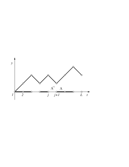
FIG. 1.: Random walk correspondance of the distribution of couplings.

The distribution of the couplings in a sample can be put in correspondence with a RW, $y(t)$, the time axis $t$ corresponding to the position $j$ along the spin chain. As shown in Fig. 1, the walker starts at $y=0$, its $j$-th step is in the positive (negative) $y$-direction when $J_{j}=\Lambda$ ($\Lambda^{-1}$) and absorbing boundary conditions are assumed for $y<0$. As a consequence, the surface magnetization of a sample is nonvanishing only when the corresponding walk survives until $t=L$, i.e., if it never crosses the time axis during $L-1$ steps. Thus the fraction of $L$-step surviving walks, $\left.P_{\rm surv}(t)\right|_{t=L}\sim L^{-1/2}$, gives the fraction of rare events for which a sample has a nonvanishing surface magnetization. Since the average value of the surface magnetization is determined by the rare events, we have the correspondence: $[m_{s}(L)]_{\rm{av}}\sim\left.P_{\rm surv}(t)\right|_{t=L}\sim L^{-1/2}$ from which the value of the critical exponent $x_{s}=\beta_{s}/\nu=1/2$ follows, in agreement with Eq. (3).

Let us consider the average of the logarithm of the products in Eq. (24) which may be written as

$$\left[\ln\prod_{j=1}^{l}\left({h_{j}\over J_{j}}\right)^{2}\right]_{\rm av}=2\sum_{j=1}^{l}\left([\ln h_{j}]_{\rm av}-[\ln J_{j}]_{\rm av}\right)=2\delta\,l\,,$$ (29)

using the definition of the control parameter in Eq. (2). In the RW picture this quantity is proportional to the average position of the walker after $l$ steps for a free walk and vanishes at criticality. In the off-critical situation, $\delta\neq 0$, the average position of the walker grows linearly with $l$, which is equivalent to having a nonzero bias $\delta_{w}=q_{w}-p_{w}\neq 0$ where $p_{w}$ ($q_{w}$) denotes the probability that the walker makes a step in the positive (negative) $y$-direction. Thus the correspondence between RTIM and RW still applies in the off-critical situation with:

$$[m_{s}(\delta,L)]_{\rm av}\sim\left.P_{\rm surv}(\delta_{w},t)\right|_{t=L}\,,\ \ \ \delta\sim\delta_{w}\,.$$ (30)

From the known behavior of the surviving probability, one deduces the values of the RTIM critical exponents given in Eq. (3).

For the inhomogeneous RTIM the local quantum control parameter has a smooth position dependence which, at the bulk critical point, is given by $\delta(l)=-Al^{-\kappa}$ according to Eq. (8). The corresponding RW has a locally varying bias with the same type of asymptotic dependence, $\delta_{w}(l)=-A_{w}l^{-\kappa}$. Consequently the average motion of the walker is parabolic:

$$y_{p}(t)=-\sum_{l=1}^{t}\delta_{w}(l)={A_{w}\over 1-\kappa}t^{1-\kappa}\,.$$ (31)

Under the change of variable $y(t)\to y(t)-y_{p}(t)$, the surviving probability of the inhomogeneously drifted walker is also the surviving probability of an unbiased walker, however with a time-dependent absorbing boundary condition at $y(t)<-y_{p}(t)$.

The surviving probability of a random walker with time-dependent absorbing boundaries has already been studied in the mathematical[16] and physical[17, 18] literature. In a continuum approximation, it follows from the solution of the diffusion equation with appropriate boundary conditions,

$${\partial\over\partial t}P(y,t)=D{\partial^{2}\over\partial y^{2}}P(y,t)\,,\ \ P[-y_{p}(t),t]=0\,.$$ (32)

Here $P(y,t)$ is the probability density for the position of the walker at time $t$ so that the surviving probability is given by

$$P_{\rm surv}(t)=\int_{-y_{p}(t)}^{\infty}\!\!P(y,t)dy\,.$$ (33)

The behavior of the surviving probability depends on the value of the decay exponent $\kappa$. For $\kappa>1/2$, the drift of the absorbing boundary in Eq. (31) is slower then the diffusive motion of the walker, typically given by

$$y_{d}(t)\sim(Dt)^{1/2}\,,$$ (34)

thus the surviving probability behaves as in the static case. When $\kappa<1/2$, the drift of the absorbing boundary is faster than the diffusive motion of the walker and leads to a new behavior for the surviving probability. For $A_{w}>0$, since the distance to the moving boundary grows in time, the surviving probability approaches a finite limit. On the contrary, for $A_{w}<0$, the boundary moves towards the walker and the surviving probability decreases with a fast, stretched-exponential dependence on $t$. Finally, in the borderline case $\kappa=1/2$ where the drift of the boundary and the diffusive motion have the same dependence on $t$, like in the static case the surviving probability decays as a power, $P_{\rm surv}(\delta_{w},t)\sim t^{-\theta(A_{w})}$, however with a continuously varying critical exponent.

Now turning back to the problem of the inhomogeneous RTIM, the RW analogy can be used to formulate a relevance-irrelevance criterion: According to the preceding discussion, the inhomogenous surface disorder is a relevant (irrelevant) perturbation for the surface critical properties of the RTIM when $\kappa<1/2$ ($>1/2$) and a marginal one when $\kappa=1/2$.

IV Results

In this Section we study the surface critical properties of the inhomogeneous RTIM, considering the size-dependence at criticality as well as the $\delta$-dependence for various quantities. We treat successively relevant and marginal perturbations and close with a discussion of the behavior in the Griffiths phase.

In the numerical calculations we used up to $5\;10^{4}$ realizations of disorder with chain sizes up to $L=2^{7}$ except for the surface magnetization for which we used up to $10^{6}$ realizations with system sizes up to $L=2^{14}$.

A Critical behavior with relevant inhomogeneity

Let us first consider the probability distribution of $\ln m_{s}$ on finite samples with length $L$ at the bulk critical point $\delta=0$. According to Eq. (28), $[\ln m_{s}]_{\rm av}$ is expected to scale as $[\ln\prod_{l=1}^{L}(J_{l}/h_{l})]_{\rm av}$ when the perturbation tends to reduce the surface order, i.e., when $A<0$ in Eq. (8). Thus one obtains:

$$[\ln m_{s}]_{\rm av} \sim \sum_{l=1}^{L}([\ln J_{l}]_{\rm av}-[\ln h_{l}]_{\rm av}$$ (35)

$$= A\sum_{l=1}^{L}l^{-\kappa}\sim AL^{1-\kappa}\,.$$ (36)

The typical magnetization, define through $[\ln m_{s}]_{\rm av}=\ln[m_{s}]_{\rm typ}$, has a stretched-exponential behavior, $[m_{s}]_{\rm typ}\sim\exp({\rm const}\,AL^{1-\kappa})$, when $A<0$. For the probability distribution of $\ln m_{s}$, Eq. (36) suggests the following scaling form:

$$P_{m}(\ln m_{s},L)={1\over L^{1-\kappa}}\tilde{P}_{m}\left[{\ln m_{s}\over L^{1-\kappa}}\right]\,.$$ (37)

Indeed, as shown in Fig. 2, the numerical results are in agreement with Eq. (37).

The asymptotic behavior of the scaling function $\tilde{P}_{m}(v)$ as $v\to 0$ depends on the signe of $A$. For enhanced surface couplings, $A>0$, there is a nonvanishing surface magnetization at the bulk critical point as $L\to\infty$, thus the powers of $L$ in Eq. (37) must cancel as seen in Fig. 2 and $\lim_{v\to 0}\tilde{P}_{m}(v)\sim v^{-1}$ so that $P_{m}(\ln m_{s})\sim 1/\ln m_{s}$. For reduced surface couplings, $A<0$, $\lim_{v\to 0}\tilde{P}_{m}(v)=0$, indicating a vanishing surface magnetization.

FIG. 2.: Probability distribution of $\ln m_{s}$ obtained for the binary distribution with $\kappa=1/4$ for $A=0.4$ and scaling plot for $A=-0.4$ (inset) for chain sizes $L=2^{10},2^{11},2^{12}$.

Next we calculate the average behavior of the surface magnetization, which is determined by the rare events with $m_{s}=O(1)$. Here we use the RW description of Section III. Starting with $A\sim A_{w}>0$, for $A_{w}\ll 1$ one defines the time scale $t^{*}$ for which the parabolic and diffusive lengths in Eqs. (31) and (34) are of the same order, $y_{p}(t^{*})\sim y_{d}(t^{*})$, such that $t^{*}\sim A_{w}^{-2/(1-2\kappa)}$. The surviving probability can be estimated by noticing that, if the walker is not absorbed up to $t^{*}$, it will later survive with a finite probability. Thus $P_{\rm surv}(A_{w}>0)\sim(t^{*})^{-1/2}\sim A_{w}^{1/(1-2\kappa)}$ and the average surface magnetization has the same behavior at the bulk critical point:

$$[m_{s}]_{\rm av}\sim A^{1/(1-2\kappa)},\ \ \kappa<\frac{1}{2},\ \ 0<A\ll 1.$$ (38)

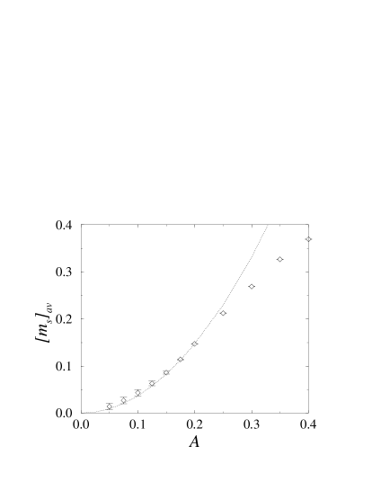
FIG. 3.: Average surface magnetization as a function of the inhomogeneity parameter for the binary distribution with $\kappa=1/4$, extrapolated at infinite size. The dotted line corresponds to the asymptotic expression in Eq.(38).

This result is in agreement with the numerical calculations as shown in Fig. 3. The error bars give the precision of the extrapolation procedure.

In the case of a shrinking interval between the walker and the absorbing wall, $A_{w}<0$, the leading behavior of the surviving probability can be estimated by looking for the fraction of walks with $y(t)>-y_{p}(t)$ which is given by $P_{\rm surv}(t)\sim\exp[-{\rm const}\,A_{w}^{2}\,t^{1-2\kappa}]$. Thus, for reduced surface couplings, the average surface magnetization has the following finite-size behavior at the critical point:

$$[m_{s}]_{\rm{av}}\sim\exp\left(-{\rm const}\,A^{2}\,L^{1-2\kappa}\right),\kappa<\frac{1}{2},A<0\,.$$ (39)

Numerical results are shown in Fig. 4. One can notice that even for such large system size as $L=2^{9}$ the linear asymptotic regime is not completely reached. One may notice the different size dependence of the typical and average surface magnetizations at criticality in Eqs. (37) and (39), respectively.

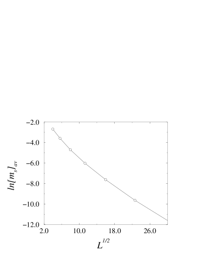
FIG. 4.: $\ln[m_{s}]_{\rm{av}}$ as a function of $L^{1-2\kappa}$ for the binary distribution with $\kappa=1/4$ and $A=-0.4$. The asymptotic linear dependence is in agreement with Eq.(39).

To obtain the $\delta$-dependence of the average surface magnetization in the thermodynamic limit, we first determine the typical size of the surface region $l_{s}$ which is affected by the inhomogeneity for $\delta<0$ and $A<0$. It is given by the condition that quantum fluctuation ($\sim\delta$) and inhomogeneity ($Al^{-\kappa}$) contributions to the energy are of the same order, from which the relation $l_{s}\sim|A|^{1/\kappa}|\delta|^{-1/\kappa}$ follows. Inserting $L\sim l_{s}$ in Eq. (39), we obtain

$$[m_{s}]_{\rm{av}}\sim\exp[-{\rm const}\,|A|^{1/\kappa}\,|\delta|^{-(1-2\kappa)/\kappa}],\kappa<\frac{1}{2},A<0,$$ (40)

as quoted in Table I. The numerical verification of this result is difficult since, close to the critical point, one has to use large finite samples, $L\gg l_{s}$, for which $[m_{s}(\delta,A)]_{\rm{av}}$ is quite small.

Let us now study the behavior of the energy gap $\epsilon_{1}(L)\sim\tau_{r}^{-1}$. Here we make use of the relation (28) between the gap and the surface magnetizations, from which the typical finite-size-scaling behavior $\ln\epsilon_{1}(L)\sim L^{1-\kappa}$ follows, as for the surface magnetization. Thus the relation between the time and length scales is

$$\ln\tau_{r}\sim\xi^{1-\kappa}\,,$$ (41)

and the probability distribution of the gap is

$$P_{\epsilon}(\ln\epsilon_{1},L)={1\over L^{1-\kappa}}\tilde{P}_{\epsilon}\left[{\ln\epsilon_{1}\over L^{1-\kappa}}\right]\,,$$ (42)

to be compared to the distribution of the surface magnetization in Eq. (37). Numerical results shown in Fig. 5 are in agreement with this scaling result.

FIG. 5.: Scaling plot of the probability distribution of the gap for the binary distribution with $A=0.5$ and $\kappa=1/4$.

In order to obtain an estimate for the average surface autocorrelation function one may notice that the disorder being strictly correlated along the time axis, a sample with a finite surface magnetization $m_{s}=O(1)$ has also a nonvanishing surface autocorrelation function $G_{s}(\tau)\sim m_{s}^{2}$. Since the fraction of rare events are the same for the two quantities, the scaling behavior of $[G_{s}(L,\tau)]_{\rm{av}}$ can be deduced from the corresponding relations for the average surface magnetization. For enhanced surface couplings, $A>0$, according to Eq. (38), $\lim_{\tau\to\infty}[G_{s}(\tau)]_{\rm{av}}\sim[m_{s}(A)]_{\rm{av}}\sim A^{1/(1-2\kappa)}$ at criticality. For reduced surface couplings, $A<0$, the finite-size critical behavior follows from Eq. (39) with $\lim_{\tau\to\infty}[G_{s}(L,\tau)]_{\rm av}\sim[m_{s}(L,A)]_{\rm av}\sim\exp[-{\rm const}\,A^{2}\,L^{1-2\kappa}]$. Now, using the scaling relation (41), we obtain

$$[G_{s}(\tau)]_{\rm av}\sim\exp\left[-{\rm const}\,A^{2}\,(\ln\tau)^{1-2\kappa\over 1-\kappa}\right]\,$$ (43)

in the thermodynamic limit. This enhanced power-law decay is consistent with the numerical results, as shown in Fig. 6.

FIG. 6.: Average surface autocorrelation function for the uniform distribution with $\kappa=1/4$ and $A=-0.5$. The solid straight line is a guide for the eye.

B Critical behavior with marginal inhomogeneity

In the borderline case, $\kappa=1/2$, several results in the previous Section have to be modified. We start with the analysis of the average surface magnetization. For the extreme binary distribution, with $\Lambda\to\infty$ in Eq. (10), there is a one-to-one correspondence between samples with a nonvanishing surface magnetization and RW’s with surviving character, as explained in Section III. Thus for this distribution one can deduce $\beta_{s}$ from the corresponding behavior of the surviving probability in the RW problem. The differential equation with absorbing boundary conditions in Eq. (32) can be solved[18] for $\kappa=1/2$ in terms of parabolic cylinder functions of order $\nu$, $D_{\nu}(x)$.[19] For zero bulk bias, $\delta_{w}=0$, the surviving probability has the asymptotic dependence $P_{\rm surv}(t)\sim t^{-\theta}$ and the exponent $\theta$ is such that

$$D_{2\theta}(-2A_{w})=0\,,$$ (44)

taking $D=1/2$ for the diffusion constant in Eq. (32). In the limiting cases the solution takes the form

$$\theta={1\over 2}-\sqrt{{2\over\pi}}\,A_{w}$$ (45)

for $|A_{w}|\ll 1$ while for large values of $A_{w}$ one obtains asymptotically:

$$\theta=\sqrt{{2\over\pi}}\,A_{w}\exp[-2A_{w}^{2}]\,.$$ (46)

Then the correspondence of Eq. (30) leads to the scaling dimension of the average surface magnetization,

$$x_{m}^{s}={\beta_{s}\over\nu}=\theta(A_{w})\,,$$ (47)

where the average correlation length exponent $\nu=2$ and $A_{w}=A_{b}$ for the extreme binary distribution.

For other inhomogeneous distributions, like in Eqs. (10) and (17), one has to find the relation between the parameter of the walk $A_{w}$ and that of the RTIM $A$. The argument goes as follows: At the bulk critical point, we compare the integrated change in the control parameter induced by the perturbation at a length scale $l$, $\Delta(l)=\sum_{j=1}^{l}[\ln J_{j}-\ln h_{j}]_{\rm av}$ to its fluctuation characterized by $\Gamma^{2}(l)=\sum_{j=1}^{l}[(\ln J_{j}-\ln h_{j})^{2}]_{\rm av}$. The dimensionless ratio $\Delta(l)/\Gamma(l)$ is equal to $2A_{b}$ and $\sqrt{2}A_{u}$ for the binary and the uniform distribution, respectively. Since it does not depend on the value of $\Lambda$ for the binary distribution and since $A_{w}=A_{b}$ when $\Lambda\to\infty$, we can identify this ratio to $2A_{w}$ which gives:

$$A_{w}=\left\{\begin{array}[]{ll}A_{b}&\ \ \mbox{binary distribution}\\ {A_{u}/\sqrt{2}}&\ \ \mbox{uniform distribution}\end{array}\right.\,.$$ (48)

FIG. 7.: Surface magnetic exponent as a function of the inhomogeneity parameter $A_{w}$. The line is a guide for the eye.

The surface magnetization exponent thus depends on the distribution, however only through the value of the parameter $A_{w}$ entering in Eq. (47), the functional form remaining the same. The average magnetization has been obtained numerically for the binary and the uniform distribution using $2\;10^{5}$ realizations of disorder for chain sizes $L=2^{5}$ to $2^{14}$. The exponents $x_{m}^{s}$ were deduced from an extrapolation of two-points approximants using the BST algorithm[20]. The results are shown in Fig. 7. The exact points in the figure are obtained by solving Eq. (44) for integer and half-integer values of $\theta$ where the parabolic cylinder functions are related to Hermite polynomials[19]. The corresponding $A_{w}$ values are then given by the highest negative zeros of the Hermite polynomial, ${\rm He}_{2\theta}(-2A_{w})=0$. For $x_{m}^{s}=0$, $A_{w}$ is shifted to $+\infty$ as it can be seen in Eq. (46). Thus the system does not display surface order at criticality as it is the case for the HvL model for sufficiently enhanced surface couplings.

Next we discuss the properties of the probability distribution of $\ln m_{s}$. Repeating the argument used above for relevant perturbations, we arrive to the scaling form of Eq. (37), however with $\kappa=1/2$. We note that the same scaling form remains valid for irrelevant perturbations, with $\kappa>1/2$, but the scaling function $\tilde{P}_{m}(v)$ has different limiting behaviors when $v\to 0$ in the two cases. While for $\kappa>1/2$ it approaches a constant, in the marginal case it goes to zero as $\lim_{v\to 0}\tilde{P}_{m}(v)\sim v^{-2x_{m}^{s}(A)+1}$. In this way one obtains the proper scaling behavior for the average surface magnetization. The numerical results in Fig. 8 are in agreement with this limiting behavior.

FIG. 8.: Scaling plot of the probability distribution of $\ln m_{s}$ for the binary distribution with $\kappa=1/2$ for chain sizes $L=2^{10},2^{11},2^{12}$.

For the distribution of the energy gap at the critical point, one can also repeat the reasoning used for the relevant case and both the distribution function in Eq. (42) and the scaling relation in Eq. (41) stay valid, with $\kappa=1/2$.

The asymptotic behavior of the average surface autocorrelation function can be determined at criticality by scaling considerations like in a previous work for the homogeneous case.[5] Here we make use of the fact that, as already explained for relevant perturbations, the average autocorrelation function has the same scaling properties as the average surface magnetization. Under a scaling transformation when lengths are rescaled by a factor $b>1$, such that $l^{\prime}=l/b$, the average surface autocorrelation behaves as

$$[G_{s}(\ln\tau)]_{\rm{av}}=b^{-x_{m}^{s}}[G_{s}(\ln\tau/b^{1/2})]_{\rm{av}}\,,$$ (49)

where we used Eq. (41) to relate the time and length scales. Taking now $b=(\ln\tau)^{2}$ we obtain:

$$[G_{s}(\tau)]_{\rm{av}}\sim(\ln\tau)^{-2x_{m}^{s}}\sim(\ln\tau)^{-\beta_{s}(A)}\,.$$ (50)

The last expression follows from the exponent relation in Eq. (47) where the average correlation length exponent is $\nu=2$. This scaling behavior has also been verified by numerical calculations as shown in Fig. 9.

FIG. 9.: Average surface autocorrelation function for the binary distribution in the marginal case with $A=0.5$. The solid straight line gives the expected scaling behavior in Eq. (50).

C Griffiths phase

In the Griffiths phase, on the paramagnetic side of the critical point, the dynamical properties of random quantum systems are anomalous. As a consequence of the so-called Griffiths-McCoy singularities,[21] the different dynamical properties can be characterized by one single parameter, the dynamical exponent $z(\delta)$, which is a continuous function of the quantum control parameter given in Eq. (7) for the homogeneous RTIM. Here we calculate $z(\delta)$ for the inhomogeneous RTIM by considering the singular behavior of two quantities: First the probability distribution of the gap and then the asymptotic behavior of the surface autocorrelation function.

From the distribution of the first gap one can deduce the dynamical exponent through the asymptotic relation:[6]

$$\lim_{\epsilon_{1}\to 0}{\ln\left[P(\ln\epsilon_{1})\right]\over\ln\epsilon_{1}}={1\over z(\delta)}\,.$$ (51)

As shown in Fig. 10 the log-log plots of the distributions obtained for different decay parameters $\kappa$, corresponding to relevant and marginal perturbations, have approximately the same slopes. Consequently, the dynamical exponent $z(\delta)$ is independent of the inhomogeneity. Similar results are obtained with the probability distributions of the second gap, which is expected to obey the same scaling relation as in Eq. (51), however with an exponent $z^{\prime}(\delta)=z(\delta)/2$.[8] As shown in Fig. 10, the probability distribution of the second gap is also insensitive to the presence of the inhomogeneity and the value of the exponent $z^{\prime}(\delta)$, deduced from the slope, is in good agreement with the analytical result in Eq. (7) with $A=0$.

FIG. 10.: Probability distribution of the first and second gaps in the Griffiths phase with the uniform distribution at $h_{0}=3$ and $A=0.5$ for different values of $\kappa$. The asymptotic slopes of the curves, obtained by least square fits, are given in parentheses.

Next we study the average surface autocorrelation function, the decay of which is connected to $z(\delta)$ through Eq. (6).

FIG. 11.: Average surface autocorrelation function in the Griffiths phase with the uniform distribution at $h_{0}=3$, $A=0.5$ and for different values of $\kappa$. The asymptotic slopes of the curves are given in parentheses.

As shown in Fig. 11, the value of the decay exponent $z(\delta)$ has only a weak dependence of the inhomogeneity exponent $\kappa$, both for relevant and marginal inhomogeneities, due to the finite size effects which are expected to be larger when $\kappa$ is decreasing. Since the variation of $z$ with the inhomogeneity is decreasing when the size of the system increases, we expect that the surface autocorrelations are also asymptotycally independent of $\kappa$. The value of $z(\delta)$ is consistent with that obtained from the distribution of the gap and corresponds to the analytical bulk result in Eq.(7).

Thus we conclude that the presence of inhomogeneous disorder does not modify the form of the Griffiths-McCoy singularities and the dynamical exponent of the inhomogeneous RTIM is the same as for the homogeneous one.

V Discussion

In this paper the influence of an inhomogeneous distribution of the disorder in the vicinity of the surface of the RTIM has been studied. We considered a random version of the HvL model where, on the average, the perturbation decays as a power $l^{-\kappa}$ of the distance $l$ from the surface. The effect of the inhomogeneity was found to be relevant (irrelevant) for $\kappa<1/2$ ($\kappa>1/2$).

The relevance-irrelevance criterion, which was shown to follow from a simple RW argument, can be generalized by making use of a more traditional approach.[22] Near the bulk critical point, the charateristic length scale of the unperturbed system is set by the average correlation length $\xi\sim\delta^{-\nu}$. The strength of the perturbation at a length scale $l$ is measured by the mean change of the control parameter, $\overline{\delta}_{A}(l)=1/l\sum_{j=1}^{l}Al^{-\kappa}\sim Al^{-\kappa}$. This has to be compared, at the scale of the correlation length $\xi$, to the deviation from the critical point $\delta$. Forming the ratio $\overline{\delta}_{A}(\xi)/\delta\sim A\xi^{-\kappa+1/\nu}$, we verify that the relative strength of the perturbation diverges (vanishes) at the critical point when $\kappa<1/\nu$ ($\kappa>1/\nu$). For the RTIM this is equivalent to the RW result of Section III since $\nu=2$ in this case.

Our next remark concerns correlated disorder in the RTIM, when the distribution of the couplings and/or transverse fields at different sites are algebraically correlated with, for example, $\langle\pi_{l}(J)\pi_{l+r}(J)\rangle\sim r^{-\omega}$. This type of correlated disorder has been recently studied in Ref.[23]. The relevance-irrelevance criterion has the same form as for inhomogeneous disorder with $\omega$ playing the role of $\kappa$. Also the relation between relevant time and length scales, $\ln\tau_{r}\sim\xi^{1-\omega}$, corresponds to the relation in Eq. (41) for relevant inhomogeneities. However the form of the critical singularities for the bulk and surface magnetizations are different in the two models.

We close this Section with a discussion of a related problem, namely, the persistence probability, $P_{\rm per}$, for a RW in an inhomogeneous one-dimensional random environment which is an inhomogeneous version of Sinai’s model.[24] The transition probabilities, $w_{l,l+1}\neq w_{l+1,l}$, are random variables and the corresponding probability distributions are inhomogeneous near the starting point of the walk, $l=1$, deviating from the bulk distributions by an amount of order $l^{-\kappa}$. We make use of an exact mapping[7, 25] between the eigenvalue problem for the fermionic excitations of the RTIM in Eq. (23) and the eigenvalue problem for the master equation of the RW, with the following correspondences:

$$w_{l,l+1} \leftrightarrow J_{l}^{2}$$ (52)

$$w_{l,l-1} \leftrightarrow h_{l}^{2}$$ (53)

$$P_{\rm per}(L) \leftrightarrow m_{s}^{2}(L)$$ (54)

$$\lambda_{\rm min} \leftrightarrow -\epsilon_{1}^{2}(L)\,.$$ (55)

Here $\lambda_{\rm min}$ is the leading eigenvalue of the Fokker-Planck operator, $L$ is the size of the system with free boundary conditions for the RTIM, whereas we take absorbing boundary conditions at both ends for the RW. Using the relations in Eq. (55), one can easily translate the results of Section IV. The inhomogeneity is relevant (irrelevant) for the diffusive and persistence properties of the RW for $\kappa<1/2$ ($\kappa>1/2$). In the case of a relevant inhomogeneity with zero global bias, the persistence probability is either finite, for locally enhanced transition probabilities to the right, or it vanishes as

$$\left[P_{\rm per}(L)\right]_{\rm av}\sim\exp\left(-{\rm const}\,L^{1-2\kappa}\right)\,,$$ (56)

for locally enhanced transition probabilities to the left.The relation between time and length scales, $\ln t\sim L^{1-\kappa}$, leads to:

$$\left[P_{\rm per}(t)\right]_{\rm{av}}\sim\exp\left[-{\rm const}\,(\ln t)^{(1-2\kappa)/(1-\kappa)}\right]\,.$$ (57)

For marginal inhomogeneity the average persistence is given by

$$\left[P_{\rm per}(t)\right]_{\rm{av}}\sim(\ln t)^{2\theta(A)}\,,$$ (58)

where the continuously varying exponent $\theta(A)$ is obtained as the solution of Eq. (44).

- [1] Permanent address: Institute for Theoretical Physics, Szeged University, H-6720 Szeged, Hungary.
- [2] For a review, see H. Rieger and A. P. Young, in Complex Behavior of Glassy Systems, edited by M. Rubi and C. Perez-Vicente, Lecture Notes in Physics Vol. 492 (Springer-Verlag, Heidelberg, 1997), p. 256.
- [3] D. S. Fisher, Phys. Rev. Lett. 69, 534 (1992); Phys. Rev. B 50, 3799 (1994); 51, 6411 (1995).
- [4] F. Iglói and H. Rieger, Phys. Rev. Lett. 78, 2473 (1997).
- [5] H. Rieger and F. Iglói F, Europhys. Lett. 39, 135 (1997).
- [6] F. Iglói and H. Rieger, Phys. Rev. B 57 11 404 (1998).
- [7] F. Iglói and H. Rieger, Phys. Rev. E 58, 4238 (1998).
- [8] F. Iglói, R. Juhász, and H. Rieger, Phys. Rev. B **, *** (1999).
- [9] A. P. Young and H. Rieger, Phys. Rev. B 53, 8486 (1996); R. H. McKenzie, Phys. Rev. Lett. 77, 4804 (1996); A. P. Young, Phys. Rev. B 56, 11691 (1997); P. Henelius and S. M. Girvin, ibid. 57, 11457 (1998); D. S. Fisher and A. P. Young, ibid. 58, 9131 (1998).
- [10] H. J. Hilhorst and J. M. J. van Leeuwen, Phys. Rev. Lett. 47, 1188 (1981); H. W. J. Blöte and H. J. Hilhorst, ibid. 51, 20 (1983); T. W. Burkhardt, I. Guim, H. J. Hilhorst, and J. M. J. van Leeuwen, Phys. Rev. B 30, 1486 (1984); H. W. J. Blöte and H. J. Hilhorst, J. Phys. A 18, 3039 (1985); T. W. Burkhardt and F. Iglói, ibid. 23, L633 (1990).
- [11] F. Iglói, I. Peschel, and L. Turban, Adv. Phys. 42 683 (1993).
- [12] E. Lieb, T. Schultz, and D. Mattis, Ann. Phys. (N.Y.) 16, 407 (1961); S. Katsura, Phys. Rev. 127, 1508 (1962); P. Pfeuty, Ann. Phys. (Paris) 57, 79 (1970).
- [13] F. Iglói and L. Turban, Phys. Rev. Lett. 77, 4804 (1996).
- [14] I. Peschel, Phys. Rev. B 30, 6783 (1984).
- [15] F. Iglói, L. Turban, D. Karevski, and F. Szalma, Phys. Rev. B 56 11 031 (1997).
- [16] K. Uchiyama, Z. Wahrsch. verw. Gebiete 54, 75 (1980); H. E. Daniels, J. Appl. Prob. 6, 399 (1969); P. Salminen, Adv. Appl. Prob. 20, 411 (1988).
- [17] L.Turban, J. Phys. A 25 L127 (1992).
- [18] P. L. Krapivsky and S. Redner, Am. J. Phys. 64, 546 (1996).
- [19] M. Abramowitz and I. A. Stegun, Handbook of Mathematical Functions, (Dover, New York, 1965).
- [20] R. Bulrisch and J. Stoer, Num. Math. 6, 413 (1964); M. Henkel and G. Schütz, J. Phys. A 21 2617 (1988).
- [21] R. B. Griffiths, Phys. Rev. Lett. 23, 17 (1969); B. McCoy, ibid. 23 383 (1969).
- [22] R. Cordery, Phys. Rev. Lett. 48 215 (1982); T. W. Burkhardt, ibid. 48 216 (1982).
- [23] H. Rieger and F. Iglói (to be published).
- [24] Ja. G. Sinai, Theor. Probab. Appl. 27, 247 (1982).
- [25] F. Iglói, L. Turban, and H. Rieger, Phys. Rev. E 59 1465 (1999).