Molecular dynamics calculation of the thermal conductivity
of vitreous silica

Abstract

We use extensive classical molecular dynamics simulations to calculate the thermal conductivity of a model silica glass. Apart from the potential parameters, this is done with no other adjustable quantity and the standard equations of heat transport are used directly in the simulation box. The calculations have been done between 10 and 1000 Kelvin and the results are in good agreement with the experimental data at temperatures above 20K. The plateau observed around 10K can be accounted for by correcting our results taking into account finite size effects in a phenomenological way.

I Introduction

The thermal properties of glasses exhibit some specific and unusual features which are well known for quite some time [1]. These features are apparent in the specific heat and the thermal conductivity but we would like to focus here on the thermal conductivity $\kappa$. The temperature dependence of $\kappa(T)$ can be separated in 3 distinct temperature domains:
- At very low temperature ($T\leq 1$K) the thermal conductivity increases like $T^{2}$. This increase can be explained within the tunneling model [2] which has been proposed almost thirty years ago.
- At intermediate temperatures ($2\leq T\leq 20$K) the thermal conductivity exhibits a “plateau” for which several explanations have been given [3]. An extension of the tunneling model, the soft-potential model, has been proposed and gives a coherent description of the plateau by introducing the concept of “soft vibrations” [4, 5].
- At high temperature, ($T\geq 30$K), $\kappa(T)$ rises smoothly and seems to saturate to a limiting value $\kappa_{\infty}$ unlike crystals where $\kappa(T)\sim 1/T$ at elevated temperature. Recently this second rise of the thermal conductivity has also been explained within the soft-potential model [6] which appears to be able to account for all the thermal anomalies of glasses over the whole temperature range.
Our aim here is not to propose a new or alternative explanation of the above mentioned anomalies. The purpose is to perform a molecular dynamics (MD) simulation on a model silica glass using a very widely used interaction potential (the so-called “BKS” potential [7]) without any pre-conception of the model able to explain the thermal anomalies of silica. This means that we do not add or inject an a priori quantity in the potential to reproduce a specific model. We use the standard definition of the heat transport coefficients that we calculate directly in our simulation box. In fact we introduce artificially inside the system a “hot” and a “cold” plate which therefore induce a heat flux. This flux creates a temperature gradient and once the steady state has been reached we can determine the thermal conductivity. By using plates compatible with the periodic boundary conditions we are able to calculate the thermal conductivity directly during the simulations without any additional parameter. This technique has been inspired by earlier studies [8] in which the plates were treated like hard walls and has mainly been applied to the calculation of the thermal conductivity in 1- or 2-dimensional systems [9, 10]. Nevertheless very recently Oligschleger and Sch$\ddot{o}$n applied the same method in a study of heat transport phenomena in crystalline and glassy samples (mainly selenium) [11]. In parallel to these studies which can be called in situ, other methods relying on the use of the density and heat flux correlation functions [12] or on the Kubo and Greenwood-Kubo formalism [13] have been developed in order to determine the thermal conductivity of solids. Our results for the thermal conductivity obtained with the BKS potential compare reasonably well with the experimental data. First of all the order of magnitude is correct above 20K and, at least in the range 20K-400K, a nice quantitative agreement is obtained. Furthermore, by taking care of finite-size corrections in a very simple phenomenological way, we are able to reproduce the plateau around 10K. Of course, the very low temperature $T^{2}$ behavior, which is known to be due to quantum effects, is out of the scope of such a classical calculation.
This paper is organized in the following way. In section II we describe the modus operandi we have used to obtain the thermal conductivity. In section III we present first the results obtained directly from the MD simulations. Then we show the effect of finite-size corrections on these results and discuss our findings. In section IV we draw the major conclusions.

II Modus Operandi

Except the determination of $\kappa(T)$, the simulations are standard classical MD calculations on a microcanonical ensemble of 648 particles (216 SiO₂ molecules) interacting via the BKS potential. Like in a previous study [14] the particles are packed in a cubic box of edge length $L=21.48$Å (the density is approximately equal to 2.18g/cm³) on which periodic boundary conditions are applied to simulate a macroscopic sample. The equations of motion are integrated using a fourth order Runge-Kutta algorithm with a time step $\Delta t$ equal to $0.7$fs. The glassy samples are obtained after a quench from the liquid state ($T\approx 7000$K) at a constant quenching rate of $2.3\times 10^{14}$K/s.
The principle of the thermal conductivity determination is illustrated in Fig.1. We consider two plates $P_{-}$ and $P_{+}$ perpendicular to the Ox axis and located at $x=-L/4$ and $x=+L/4$. These plates have a width $2\delta$ along Ox and their surface is $L^{2}$. The positions of these plates permit to keep the periodic boundary conditions without introducing an asymmetry in the system. This has the advantage, compared to other studies [15] in which the introduction of the thermostatic plates breaks the symmetry, to use a relatively small number of particles. At each iteration the particles which are inside $P_{-}$ and $P_{+}$ are determined and their number is respectively $N_{-}$ and $N_{+}$. Once these particles are determined a constant energy $\Delta\epsilon$ is subtracted from the energy of the particles inside $P_{-}$ and added to the energy of the particles in $P_{+}$. By imposing the heat transfer in this manner we insure a constant heat flux per unit area $J_{x}$ [16] which is equal to $\Delta\epsilon/(2L^{2}\Delta t)$. (the factor 2 comes from the fact that the heat flux coming from the hot plate splits equally into two parts to reach the cold plate). The energy modification is done by rescaling the velocities of the particles inside the plates. Nevertheless to avoid an artificial drift of the kinetic energy this has to be done with the total momentum of the plates being conserved. For a particle $i$ inside $P_{-}$ or $P_{+}$ the modified velocity is given at each iteration by

$$\vec{v_{i}}^{\prime}=\vec{v_{G}}+\alpha(\vec{v_{i}}-\vec{v_{G}})$$ (1)

where $\vec{v_{G}}$ is the velocity of the center of mass of the ensemble of particles in the plate and

$$\alpha=\sqrt{1\pm\frac{\Delta\epsilon}{E_{c}^{R}}}$$ (2)

depending on whether the particles are inside $P_{+}$ or $P_{-}$. The relative kinetic energy $E_{c}^{R}$ is given by

$$E_{c}^{R}=\frac{1}{2}\sum_{i}m_{i}\vec{v_{i}}^{2}-\frac{1}{2}\sum_{i}m_{i}\vec{v_{G}}^{2}$$ (3)

Following the standard definition of the transport coefficients [16] the thermal conductivity is given by

$$\kappa=-\frac{J_{x}}{\partial T/\partial x}$$ (4)

where $\partial T/\partial x$ is the temperature gradient along Ox. This formula, known as the Fourier’s law of heat flow, is only valid when a stable, linear temperature profile is obtained in the system. To calculate the gradient we divide the simulation box into $N_{s}$ “slices” along Ox in which the temperature is calculated at each iteration. Due to the periodic boundary conditions we can concentrate only on the $N_{s}/2$ slices between $x=-L/4$ and $x=L/4$ and have a better determination of the temperature in these slices since by symmetry arguments these slices are equivalent to the $N_{s}/2$ slices located outside $[-L/4,L/4]$. We can therefore determine the temperature $T_{i}$ ($i=1,..N_{s}/2$) of each slice at each iteration. By averaging each $T_{i}$ over a large number of iterations to kill the unavoidable large temperature fluctuations (due to the small average number of particles in each slice), we are able to determine after which simulation time $\tau$ the averaged profile of $T(x)$ can reasonably well be approximated by a straight line. After that time we estimate $T(x)$ using a first order least square fit of the averaged $T_{i}$’s, the slope of which will give us the temperature gradient. At that point all the quantities necessary to calculate $\kappa$ are determined.
Concerning the “practical details” of the simulation we have checked that the results are independent on the choice of $\Delta\epsilon$ and for the other quantities we have used a compromise between computer time and accuracy of the results. Here are the values used in our simulations: the width of the plates has been taken equal to $2\delta=1$Å which means that approximately 30-40 atoms are inside the plates at each iteration. The temperature gradient has been determined on $N_{s}/2=6$ slices, each slice containing approximately 100 particles. $\kappa$ has been determined on samples which have been saved all along the quenching procedure and therefore have different temperatures T. To have the same treatment for each sample we have fixed $\Delta\epsilon$ to 1% of $k_{B}T$ which appears to be a good choice. The temperature gradients obtained this way are small enough to insure the validity of Eq. 4. The most problematic choice is the simulation time $\tau$. Indeed in order to reach the steady state one needs long MD runs. For us a typical run consists of 50000 MD steps (35 ps) directly after the quench during which the average temperature is fixed and the heat transfer is switched on. Then we perform 450000 supplemental steps (315 ps) with only the heat transfer but no other constraints during which the results are collected and averaged. After this time the temperature gradient should have converged and the value of $\kappa$ should be constant. As we can see in figure 2, this can be considered to be qualitatively true for the samples above 10K but certainly not for the low temperature systems. In fact at low temperature longer runs (1 million steps (700 ps)) are necessary and still the convergence is not perfect (it is interesting to note that though our method converges slowly, it still converges faster than the calculation of $\kappa(t)$ given by a steady state experiment without a temperature gradient ([17], p.61)). It is also worth noticing that the characteristic sigmoidal shape of the temperature profile observed at 1K is consistent to what is expected in the intermediate regime where only heat transport over a small distance close to the plates is effective. In the following, only the results above 8K will be reported.

III Results

The results obtained for the thermal conductivity as a function of temperature in our model silica glass are reproduced in Fig.3 and compared to experimental data collected between 1 and 100K [18] and up to 1000K [19]. The first observation is that our simulations with the BKS potential give the correct order of magnitude over the whole temperature range (except at very low temperatures) with no adjustable parameters apart from the “technical parameters” described above and the constitutive potential parameters. At very high temperatures, say above 500K, one observes a more marked saturation of $\kappa(T)$ than in the experiments. This might be explained by the fact that other contributions than the one described here can occur in the experiments at such high temperatures. It is known that the radiative contributions (photon transport) in particular increase quickly in this temperature range and can become of the order of the phonon contributions [19]. In a large intermediate range, 20K to 400K, the agreement between the calculated and experimental values is very good. Indeed in the simulation also $\kappa$ increases in this temperature range unlike what is found in crystalline samples. The major discrepancy between the simulation and the experiment can be seen between 8 and 20K since we do not find the characteristic plateau in the thermal conductivity. In the following, we would like to argue that this discrepancy is essentially due to finite size effects.
In our cubic finite simulation box with periodic boundary conditions, the components of the $\overrightarrow{k}$ wavevectors take discrete values of the form $k_{x}=n_{x}2\pi/L$, where $n_{x}$ is a relative integer (and similarly for the other space directions), and one cannot find, in principle, propagative phonons with a frequency smaller than a lower cut-off $\omega_{c}$ which can be estimated by $2\pi v_{T}/L$, where $v_{T}$ is the transverse sound velocity. Considering the experimental value $v_{T}=3.75\times 10^{5}$ cm/s for silica[20] this gives $\omega_{c}/2\pi\simeq 1.5$ THz (in practice, when diagonalizing the dynamical matrix in our low temperature sample, we find, similarly to a previous work done on the same system [21], a slightly lower first non-zero frequency $\omega_{o}/2\pi\simeq 1.2$ THz, in agreement with the existence of an excess of modes (maybe non-propagative), the so-called Boson peak[22], in this frequency range [23]. Therefore using the correspondence $\hbar\omega=3k_{B}T$ which gives the average phonon frequency $\omega$ of the phonons excited at temperature $T$, there are certainly not enough phonons excited at temperatures below $T_{o}\simeq 19K$ in our box to be able to reproduce the experimental curve correctly. In Fig.3, the departure between our simulations and experiments is actually seen at a temperature of the order of 20K, in good agreement with this analysis.
To try to put this argument on more quantitative grounds, let us assume that the thermal conductivity is given by the usual formula [24],

$$\kappa={1\over 3}Cv\ell$$ (5)

where $C$ is the heat capacity per unit volume, $v$ and $\ell$ the velocity and mean free path of the phonons, respectively. When applying such a formula to glasses one has to be careful because of localization effects. Obviously $v$ and $\ell$ are the characteristics of the “propagative” phonons, i.e. those which really contribute to the transport phenomena. Consequently the heat capacity $C$ to be considered should be only due to the contribution of these phonons and therefore (according to other authors [2, 4]) should exhibit at low temperature the usual Debye behavior (the same as in crystals). If we assume also that the lack of phonons in our box, i.e. a wrong value of $C$, is the essential cause for the underestimated calculated value of $\kappa$, a very simple and crude way to take care of this is to multiply our simulation results by a corrective factor $C_{\infty}/C_{b}$ which can be estimated by taking for $C_{\infty}$ and $C_{b}$ the heat capacities calculated in the Debye approximation for an infinite system and a finite cubic box of edge $L$, respectively. To calculate this temperature dependent factor we have used the standard formulae[24]

$$C_{\infty}={k_{B}\over 2\pi^{2}}({1\over v_{L}^{3}}+{2\over v_{T}^{3}})\int_{0}^{\omega_{D}}\Bigl{(}{\hbar\omega/2k_{B}T\over\sinh(\hbar\omega/2k_{B}T)}\Bigr{)}^{2}\omega^{2}d\omega$$ (6)

$$C_{b}={k_{B}\over L^{3}}\sum_{p}\sum_{\overrightarrow{k}}\Bigl{(}{\hbar v_{p}k/2k_{B}T\over\sinh(\hbar v_{p}k/2k_{B}T)}\Bigr{)}^{2}$$ (7)

with $\omega_{D}^{3}=(N/L^{3})18\pi^{2}\bigl{(}1/v_{L}^{3}+2/v_{T}^{3}\bigr{)}^{-1}$. In the expression of $C_{b}$ the double sum runs over the three polarizations $p=L,T_{1},T_{2}$ and over the first $N$ $\overrightarrow{k}$ vectors (quantized as indicated above) of lowest norm $k=|\overrightarrow{k}|$. For $N$ and $L$ we have taken the simulation values $N=648$ and $L=21.48$Å and for the sound velocities the experimental values $v_{L}=5.9\times 10^{5}$ cm/s and $v_{T_{1}}=v_{T_{2}}=3.75\times 10^{5}$ cm/s [20]. When correcting our numerical data this way, we obtain the open squares represented in Fig.3 which turn out to be in very good agreement with the experimental results in the plateau region. Of course, our reasoning is very crude since it assumes that finite size corrections affect only the heat capacity contribution in the expression of $\kappa$ (Eq.5) and that the harmonic approximation holds for the propagative phonons in that temperature range, however we think that the agreement with the data cannot be fortuitous. It is unfortunate that we could not obtain more reliable results at temperatures lower than 8K (due to the impossibility to reach the permanent regime). Anyway, after correction, these results would certainly give larger values for $\kappa$ than the experiments since it is known that, at very low temperatures, the propagative phonons start to be scattered on the quantum two level systems[2] and therefore should have a lower mean free path than the one obtained in a classical calculation like the one performed here.

IV Conclusion

In conclusion we have presented the results of an extensive classical molecular dynamics simulation aimed to determine the thermal conductivity in a model silica glass. This determination has been done directly inside the MD scheme with the use of the standard equations governing the macroscopic transport coefficients and no pre-conceived model has been assumed. Moreover it turns out that this method has considerable advantages (especially concerning the length of the simulations) compared to the standard methods usually implemented to calculate the transport coefficients [17]. The calculated values of the thermal conductivity are in good agreement with the experimental data at high temperature ($T>20$K) and by including finite size corrections in a simple way we are able to reproduce the plateau in the thermal conductivity around $10$K, which has been the topic of several interpretations in the literature [3]. The agreement between the calculated and the experimental values of the thermal conductivity is even more striking when taking into account the ultra-fast quenching rate used to generate our amorphous samples. This shows once more the good quality of the BKS potential which permits to reproduce the thermal anomalies of vitreous silica with no additional parameters.
Of course, our arguments on the finite size effects should be tested in the future by running larger samples. Nevertheless the simple phenomenological correction is so efficient that one can reasonably claim that the initial discrepancy between the calculated and experimental values of the thermal conductivity is indeed due to finite size effects and not to a weakness of the method. Therefore we believe that this technique is a good way to calculate the thermal properties of materials directly inside molecular dynamics simulations.
Most of the numerical calculations have been done on the IBM/SP2 computer at CNUSC (Centre National Universitaire Sud de Calcul), Montpellier. We would like to thank Claire Levelut and Jacques Pelous for very interesting comments.

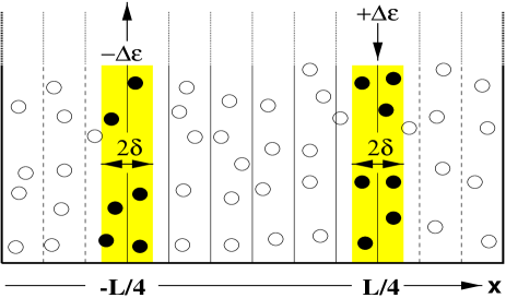
FIG. 1.: Schematic representation of the method used to determine the thermal conductivity. More details can be found in the text.

FIG. 2.: Values of the temperature as a function of $x$ in the slices located between $x=-L/4$ and $x=L/4$ for 4 different samples and the corresponding least square linear fit:
(a) $T\approx 1$K; (b) $T\approx 11$K; (c) $T\approx 27$K and (d) $T\approx 89$K.

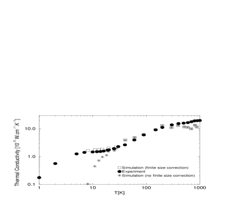
FIG. 3.: Log-log plot of the thermal conductivity as a function of temperature in silica:
$\bullet$: experiment; $\ast$: simulations; $\Box$: simulations with finite-size corrections.

REFERENCES

- [1] R. Bruckner, J. Non. Cryst. Solids, 5 123 (1970); R.C. Zeller and R.O. Pohl, Phys. Rev. B, 4 2029 (1971); D.G. Cahill and R.O. Pohl, Phys. Rev. B, 35 4067 (1987).
- [2] P.W. Anderson, B.I. Halperin and C.M. Varma, Phil. Mag., 25 1 (1972); W.A. Phillips, J. Low Temp. Phys., 7 351 (1972).
- [3] J.E. Graebner, B. Golding and L.C. Allen, Phys. Rev. B, 34, 5696 (1986); C.C. Yu and J.J. Freeman, Phys. Rev. B, 36, 7620 (1987); E. Akkermans and R. Maynard, Phys. Rev. B, 32, 7850 (1985); S. Alexander, O. Entin-Wohlman and R. Orbach, Phys. Rev. B, 34, 2726 (1986).
- [4] V.G. Karpov, M.I. Klinger and F.N. Ignat’ev, Sov. Phys. JETP, 57, 439 (1983).
- [5] M.A. Ill’in, V.G. Karpov and D.A. Parshin, Sov. Phys. JETP, 65, 165 (1987).
- [6] L. Gil, M.A. Ramos, A. Bringer and U. Buchenau, Phys. Rev. Lett., 70, 182 (1993).
- [7] B. W. H. van Beest, G. J. Kramer and R.A. van Santen, Phys. Rev. Lett., 64, 1955 (1990).
- [8] A. Tenenbaum, G. Ciccotti and R. Gallico, Phys. Rev. A, 25, 2778 (1982). R.D. Mountain and R.A. MacDonald, Phys. Rev. B, 28, 3022 (1983).
- [9] A. Maeda and T. Munakata, Phys. Rev. E, 52, 234 (1995).
- [10] J. Michalski, Phys. Rev. B, 45, 7054 (1992).
- [11] C. Oligschleger and J.C. Schn, Phys. Rev. B, to be published.
- [12] A.J.C. Ladd, B. Moran and W.G. Hoover, Phys. Rev. B, 34, 5058 (1986).
- [13] P.B. Allen and J.L. Feldman, Phys. Rev. B, 48, 12581 (1993); J.L. Feldman, M.D. Kluge, P.B. Allen and F. Wooten, Phys. Rev. B, 48, 12589 (1993)
- [14] P. Jund and R. Jullien, Phil. Mag. A, 79, 223 (1999).
- [15] H. Kaburati and M. Machida, Phys. Lett. A, 181(2), 85 (1993).
- [16] F. Reif in Fundamentals of statistical and thermal physics, McGraw-Hill (1965).
- [17] M.P. Allen and D.J. Tildesley in Computer simulation of liquids, Oxford University Press, New-York (1990).
- [18] R.B. Stephens, Phys. Rev. B, 8 2896 (1973).
- [19] J. Zarzycki in Les verres et l’état vitreux, Masson, Paris (1982) and references therein.
- [20] F. Terki, C. Levelut, M. Boissier and J. Pelous, Phys. Rev. B 53, 2411 (1996)
- [21] S.N. Taraskin and S.R. Elliott, Phys. Rev. B 55, 1 (1997).
- [22] G. Winterling, Phys. Rev. B 12, 2432 (1975); F.L. Galeener, A.J. Leadbetter and M.W. Stringfellow, Phys. Rev. B 27, 1052 (1983); U. Buchenau, H.M. Zhou, N. Nuker, K.S. Gilroyand W.A. Phillips, Phys. Rev. Lett. 60, 1318 (1988).
- [23] We do find (like other authors[21]) an excess of modes at low frequencies compared with the Debye formula when diagonalizing the dynamical matrix. However the maximum of this excess of modes is located at a frequency of about 2THz, i.e. almost twice the experimental value. We think that this discrepancy is simply due to finite size effects : by reducing the lowest frequency one would shift this maximum excess of modes to lower frequencies.
- [24] C. Kittel in Introduction à la Physique de l’état solide, Paris, Dunod, (1970).