$d_{x^{2}-y^{2}}$ Wave Pairing Fluctuations and Pseudo Spin Gap in Two-Dimensional Electron Systems

1 Introduction

In the underdoped region of high-$T_{c}$ cuprates, spin and charge excitations widely show pseudogap phenomena in the normal metallic states from temperatures $T_{PG}$ much higher than the superconducting transition temperature $T_{c}$. Influence of the pseudogap formation shows up in various different experimental probes such as NMR relaxation time, the Knight shift, neutron scattering, tunnenling, photoemission, specific heat, optical conductivity, and DC resistivity .${}^{\hbox{\immediate{\bf{?}})}}$ In particular, the angle resolved photoemission spectra (ARPES) ${}^{\hbox{\immediate{\bf{?}},\penalty 1000\hskip 0.91003pt plus 0.70004pt minus 0.70004pt{\bf{?}})}}$ have revealed that the pseudogap starts growing first in the single-particle excitations around $(\pi,0)$ and $(0,\pi)$ points at $T=T_{PG}$. With decrease in temperature, the formation of the pseudogap gradually extends in the direction of diagonal in the Brillouin zone such as $(\pi/2,\pi/2)$ and seems to continuously merge into the $d_{x^{2}-y^{2}}$ gap below $T_{c}$. From this observation, it is clear that the $(\pi,0)$ and $(0,\pi)$ regions in the single-particle excitation have a particular importance in the mechanism of the pseudogap formation because the pseudogap starts from these regions. In fact $(\pi,0)$ and $(0,\pi)$ regions are known from the ARPES data as the region where the quasiparticle dispersion is very flat with strong damping in the underdoped cuprates. This seems to suggest that the pseudogap instability is caused because of such flat and damped dispersion. We call such $(\pi,0)$ and $(0,\pi)$ momenta “flat spot” and the region around them “flat shoal region” and pay a particular attention in this paper to understand the mechanism of the pseudogap formation. We note that the flat dispersion around the flat spots is also reproduced in numerical calculations ${}^{\hbox{\immediate{\bf{?}},\penalty 1000\hskip 0.91003pt plus 0.70004pt minus 0.70004pt{\bf{?}})}}$ and plays a particularly important role in the understanding of the metal-insulator transition ${}^{\hbox{\immediate{?},\penalty 1000\hskip 0.91003pt plus 0.70004pt minus 0.70004pt{\bf{?}})}}$

A remarkable point of the pseudogap is that it appears in both of spin and charge excitations and its gap structure in the momentum space is the same as the superconducting $d_{x^{2}-y^{2}}$ symmetry with continuous evolution through $T_{c}$. This implies that the pseudogap phenomena have close connection to the superconducting fluctuations. Another somewhat puzzling point to be stressed is that although the pseudogap structure appears in $1/T_{1}T$ ,${}^{\hbox{\immediate{\bf{?}},\penalty 1000\hskip 0.91003pt plus 0.70004pt minus 0.70004pt{\bf{?}},\penalty 1000\hskip 0.91003pt plus 0.70004pt minus 0.70004pt{\bf{?}},\penalty 1000\hskip 0.91003pt plus 0.70004pt minus 0.70004pt{\bf{?}},\penalty 1000\hskip 0.91003pt plus 0.70004pt minus 0.70004pt{\bf{?}})}}$ in many cases, $1/T_{2G}$ which measures ${\rm Re}\chi(Q=(\pi,\pi),\omega=0)$ continuously increases with the decrease in temperature with no indication of the pseudogap. This implies that the antiferromagnetic excitations are suppressed below $T_{PG}$ but not in a simple fashion. A related observation is the so called resonance peak in the neutron scattering experiments .${}^{\hbox{\immediate{\bf{?}})}}$ A resonance peak above the pseudogap frequency sharply grows below $T_{c}$ or $T_{PG}$. This peak frequency $\omega^{\ast}$ decreases with decreasing doping concentration, which suggests that the resonance peak may well continuously evolve into the Bragg peak in the AFM phase. This strongly supports the idea that the AFM fluctuations are suppressed around $\omega=0$ but well retained or even enhanced at a nonzero frequency below $T_{PG}$. These observations lead to the necessity to consider the superconducting and antiferromagnetic fluctuations on an equal footing and examine their interplay in detail.

From theoretical point of view, the origin of the pseudogap is still controvertial .${}^{\hbox{\immediate{\bf{?}})}}$ It is important to understand why the pseudogap region is so wide in the underdoped region of the high-$T_{c}$ cuprates. In the weak-coupling superconductors, pairing fluctuations are usually observed only very close to $T_{c}$ and the BCS mean-field description is rather adequate. However, in the high-$T_{c}$ cuprates, the coherence length is only several lattice spacings even within a CuO₂ plane, and much smaller than the BCS superconductors. Such strong coupling nature of the pairing makes the fluctuation region wider. In addition, the quantum degeneracy temperature (coherence temperature $T_{coh}$ ) approaches zero if the Mott insulating state is approached in a continuous fashion. This necessarily leads to the vanishing $T_{c}$. In the underdoped region, such suppression of coherence becomes stronger and it could become smaller than the energy scale of the pairing force($\sim T_{PG}$). With decreasing doping concentration, if the pairing force remains finite, the separation of $T_{c}$ and $T_{PG}$ is a natural consequence.

Sometimes such suppressed $T_{c}$ far below $T_{PG}$ is modelled by the Bose condensation .${}^{\hbox{\immediate{\bf{?}},\penalty 1000\hskip 0.91003pt plus 0.70004pt minus 0.70004pt{\bf{?}},\penalty 1000\hskip 0.91003pt plus 0.70004pt minus 0.70004pt{\bf{?}},\penalty 1000\hskip 0.91003pt plus 0.70004pt minus 0.70004pt{\bf{?}},\penalty 1000\hskip 0.91003pt plus 0.70004pt minus 0.70004pt{\bf{?}})}}$ However, this strong coupling aspect cannot be well described by a simple Bose condensation, because the superconducting phase appears near the strongly correlated insulator, the Mott insulator. Because of its correlated nature which we try to clarify in this paper, the pairing fluctuations do not appear as simple bosons but as a complicated interplay with underlying metal-insulator transition, antiferromagnetic fluctuations, $d$-wave symmetry of pairing, and strong momentum dependence of single-particle excitations persisted in the pseudogap region. An important point often ignored in the literature is the vertex correction, which we discuss its effects in this paper.

In this paper, we make effort to understand the origin of the pseudo-gap behavior in AFM spin excitations. We consider the problem under the condition that both of the $d$SC and AFM fluctuations play roles in low energy scales. The pseudogap seen in the spin excitations is consistently understood from the $d$SC fluctuations and precursor effects to the $d$-wave superconductors.

One-loop renormalization group treatments of electrons around the van-Hove singular points at the Fermi level ${}^{\hbox{\immediate{\bf{?}},\penalty 1000\hskip 0.91003pt plus 0.70004pt minus 0.70004pt{\bf{?}},\penalty 1000\hskip 0.91003pt plus 0.70004pt minus 0.70004pt{\bf{?}})}}$ show the appearance of attractive vertices for the $d$SC channel as well as for the AFM, though it is difficult to discuss properties at their strong coupling fixed point from them. Learning from this insight, in § 2, we derive the low-energy effective action for the relevant AFM and $d$SC fields from the electrons around the flat spots. In § 3, mode-mode coupling terms are considered in the effective action. We apply and extend the SCR (self-consistent renormalization) theory developed by Moriya and his coworkers to improve the RPA .${}^{\hbox{\immediate{\bf{?}})}}$ In § 4, we give numerical results and their physical interpretations, and discuss the relation to the pseudogap in high-$T_{c}$ cuprates. We find two characteristic temperatures, $T_{PG}$ and $T_{\ast}$ when the $d$SC order appears at $T=0$. The spin pseudogap with suppression in $1/T_{1}T$ appears below $T_{PG}$. Below this temperature, the $d$SC correlations become dominant over the AFM correlations and the resultant decrease in the paramagnon damping takes place. The AFM correlations are still increasing with decrease in temperature in this region. Below $T_{\ast}$ the antiferromagnetic correlation starts decreasing while the pairing correlations grow as in renormalized classical regime and the superconducting transition occurs shortly. If the paramagnon damping is determined from the scattering from the flat shoal region, as expected in the underdoped region, $T_{PG}$ is substantially higher than $T_{\ast}$. In the region $T_{\ast}<T<T_{PG}$, the precursor to the superconducting state develops the pseudogap structure. When the paramagnon damping is dominantly controlled from the region other than the flat shoal region, $T_{PG}$ merges into $T_{\ast}$. These reproduce the basic features of the experimental results. § 5 is the summary of this paper and the problems left for the future are also dicussed.

2 Low-Energy Effective Action

Under the condition that AFM fluctuations are the only important ones in the long-length scale of the system, several theoretical and approximate descriptions were developed. For example, in the Mott insulating systems, Chakravarty, Halperin and Nelson developed a renormalization group scheme for the low-energy AFM exciations by employing the $d\!+\!1$-dimensional nonlinear-$\sigma$ model. .${}^{\hbox{\immediate{\bf{?}},\penalty 1000\hskip 0.91003pt plus 0.70004pt minus 0.70004pt{\bf{?}})}}$ Another quite different treatment of the AFM fluctuations in the literature is the Gaussian approximation of the paramagnetic metallic phase by starting from the Ginzburg-Landau-Wilson action in the overdamped regime due to the coupling to the Stoner excitations. ${}^{\hbox{\immediate{\bf{?}},\penalty 1000\hskip 0.91003pt plus 0.70004pt minus 0.70004pt{\bf{?}},\penalty 1000\hskip 0.91003pt plus 0.70004pt minus 0.70004pt{\bf{?}})}}$

There exist, however, more complicated cases where other type of fluctuations also come into play in the low energy scale. In this case, interplay and competition between different fluctuations seriously affect physical properties in general with possibilities of new critical phenomena. The high-$T_{c}$ cuprates provide such examples, where pairing fluctuations are expected to compete with AFM fluctuations, because AFM and dSC long-ranged ordered phases are observed close each other in the two-dimensional $T-\delta$ (temperature-hole concentration) phase diagram.

Even when one starts from the path integral with the auxiliary fields describing only the AFM fluctuations, in principle, all the other fluctuations are of course also correctly taken into account if the functional integral is performed honestly up to infinite order. In princple, it can be done by taking account all the fluctuations around the AFM saddle point. It is, however, practically not easy to handle. Physically meaningful results are rather obtained by taking account not only of the AFM saddle point but also additional contributions from other relevant saddle points separately. This procedure is justified if the overlap between fluctuations around different saddle point is properly considered to keep away from double counting of the degrees of freedom. To discuss interplay between dSC and AFM fluctuations, here, we treat the AFM and dSC saddle points and fluctuations around them on equal footing.

We consider a 2D strongly correlated electron system and assume that AFM and pairing fluctuations are both strong as in the high $T_{c}$ cuprates. The AFM fluctuations are easily taken into account in the standard functional-integral technique by the Stratonovich-Hubbard transformation for the local Coulomb repulsion, in which integrals over auxiliary fields for the AFM order parameter appear. The Stratonovich-Hubbard field for the AFM fluctuations is given by SU(2) symmetric variable ${\mbox{\boldmath$\phi$}}_{\sigma}$. At the moment the microscopic process which drives the $d$-wave pairing flucutations is not competely understood. Although we discuss below possible microscopic origins of the pairing saddle point, we first introduce $U(1)$ symmetric auxiliary field $\phi_{d}$ on phenomenologcal grounds. Then the partition function represented by the functional integral over both of the AFM and dSC auxiliary fields, ${\mbox{\boldmath$\phi$}}_{\sigma}$ and $\phi_{d}$, respectively reads

$$Z = \!\int\!{\cal D}a^{\!{}^{\dagger}}{\cal D}a{\cal D}{\mbox{\boldmath$\phi$}}_{\sigma}{\cal D}\bar{\phi_{d}}{\cal D}\phi_{d}e^{-\tilde{S}}$$ (2.1)

$$\tilde{S} = -\beta\sum_{m}\!\int\!d^{2}{\mbox{\boldmath$k$}}(i\Omega_{m}-\varepsilon_{\mbox{\boldmath$k$}})a^{\!{}^{\dagger}}_{\alpha}(i\Omega_{m},{\mbox{\boldmath$k$}})a_{\alpha}(i\Omega_{m},{\mbox{\boldmath$k$}})$$ (2.2)

$$+\beta\sum_{n}\!\int\!d^{2}{\mbox{\boldmath$q$}}{\hbox{$\left[\vbox to0.0pt{}\right.\n@space$}}2\sqrt{|\Gamma_{\sigma}|T}{\mbox{\boldmath$S$}}(i\omega_{n},{\mbox{\boldmath$q$}})\!\cdot\!{\mbox{\boldmath$\phi$}}_{\sigma}(-i\omega_{n},-{\mbox{\boldmath$q$}})+i\sqrt{|\Gamma_{d}|T}\left\{d^{\!{}^{\dagger}}(i\omega_{n},{\mbox{\boldmath$q$}})\phi_{d}(i\omega_{n},{\mbox{\boldmath$q$}})+d(i\omega_{n},{\mbox{\boldmath$q$}})\bar{\phi_{d}}(i\omega_{n},{\mbox{\boldmath$q$}})\right\}$$

$$+{\mbox{\boldmath$\phi$}}_{\sigma}(i\omega_{n},{\mbox{\boldmath$q$}})\!\cdot\!{\mbox{\boldmath$\phi$}}_{\sigma}(-i\omega_{n},-{\mbox{\boldmath$q$}})+\bar{\phi_{d}}(i\omega_{n},{\mbox{\boldmath$q$}})\phi_{d}(i\omega_{n},{\mbox{\boldmath$q$}}){\hbox{$\left]\vbox to0.0pt{}\right.\n@space$}},$$

where $a^{\!{}^{\dagger}}$ and $a$ are Grassman fields for electrons, ${\mbox{\boldmath$\phi$}}_{\sigma}$ is the three-component vector field corresponding to the spin, and $\bar{\phi_{d}}$ and $\phi_{d}$ are the pairing fields creating and annihilating a pair of electrons, respectively. $\beta$ is the inverse temperature and $\omega_{n}$ and $\Omega_{m}$ are bosonic and fermionic Matsubara frequencies. The bare dispersion is described by $\varepsilon_{\bf k}$. Here, we take the nearest-neighbor transfer $t$ and the next-nearest-neighbor transfer $t^{\prime}$, which leads to $\varepsilon_{\bf k}=-2t({\rm cos}k_{x}+{\rm cos}k_{y})-4t^{\prime}({\rm cos}k_{x}{\rm cos}k_{y}+1)-\mu$, where $\mu$ is the chemical potential measured from the flat spots. Further we have introduced the following operators corresponding to spin, and annihilating and creating a $d_{x^{2}-y^{2}}$-wave electron pair,

$${\mbox{\boldmath$S$}}(i\omega_{n},{\mbox{\boldmath$q$}}) = \sum_{m}\!\int\!d^{2}{\mbox{\boldmath$k$}}a^{\!{}^{\dagger}}_{\mu}(i\Omega_{m}-i\omega_{n},{\mbox{\boldmath$k$}}-{\mbox{\boldmath$q$}}){\mbox{\boldmath$\sigma$}}_{\mu\nu}a_{\nu}(i\Omega_{m},{\mbox{\boldmath$k$}})$$ (2.3)

$$d(i\omega_{n},{\mbox{\boldmath$q$}}) = \sum_{m}\!\int\!d^{2}{\mbox{\boldmath$k$}}a_{\mu}(i\Omega_{m},{\mbox{\boldmath$k$}})\sigma^{y}_{\mu\nu}a_{\nu}(-i\Omega_{m}+i\omega_{n},-{\mbox{\boldmath$k$}}+{\mbox{\boldmath$q$}})g({\mbox{\boldmath$k$}})$$ (2.4)

$$d^{\!{}^{\dagger}}(i\omega_{n},{\mbox{\boldmath$q$}}) = \sum_{m}\!\int\!d^{2}{\mbox{\boldmath$k$}}a^{\!{}^{\dagger}}_{\mu}(i\Omega_{m}-i\omega_{n},{\mbox{\boldmath$k$}}-{\mbox{\boldmath$q$}})\sigma^{y}_{\mu\nu}a^{\!{}^{\dagger}}_{\nu}(-i\Omega_{m},-{\mbox{\boldmath$k$}}),$$ (2.5)

where $\sigma_{\mu\nu}^{i}$ is the $i$-th component of the Pauli matrix, and $g({\mbox{\boldmath$k$}})=\cos k_{x}-\cos k_{y}$. The term containing $\Gamma_{\sigma}$ is obtained from the Coulomb interaction term by the Stratonovich-Hubbard transformation for the AFM auxiliary fields ${\mbox{\boldmath$\phi$}}_{\sigma}$ while the term containing $\Gamma_{d}$ represents coupling to the pairing auxiliary field $\phi_{d}$.

To understand the possible origin of the term containing the dSC fluctuations $\phi_{d}$ and $\bar{\phi_{d}}$, the one-loop level analyses provide a useful insight. On this level, in 2D systems, we first have to consider the contribution from the quasi-particles around $(\pi,0)$ momentum, because the $(\pi,0)$ point contribution generates the most divergent logarithmic terms due to the Umklapp scattering and also due to the van-Hove singularity. We consider two-dimensional interacting electron systems with the Fermi level being located near the flat spots, namely $(\pi,0)$ and $(0,\pi)$ points. As we mentioned in §1, these flat spots are not only the original van-Hove singular point but also the points around which flat dispersions are generically observed experimentally ${}^{\hbox{\immediate{?},\penalty 1000\hskip 0.91003pt plus 0.70004pt minus 0.70004pt{\bf{?}})}}$ as well as numerically even when the bare band structure does not suggest the van-Hove singularity at these spots .${}^{\hbox{\immediate{?},\penalty 1000\hskip 0.91003pt plus 0.70004pt minus 0.70004pt{?},\penalty 1000\hskip 0.91003pt plus 0.70004pt minus 0.70004pt{?})}}$ One-loop renormalization group theories show that at low energies, both of the $d$SC and AFM susceptibilities become divergent. In fact the $d$SC channel is most strongly divergent when the nesting conditon is not satisfied. ${}^{\hbox{\immediate{?},\penalty 1000\hskip 0.91003pt plus 0.70004pt minus 0.70004pt{?},\penalty 1000\hskip 0.91003pt plus 0.70004pt minus 0.70004pt{?})}}$ It implies that the irreducible vertices for the $d$SC and AFM channels are negative at energies low enough compared with the ultraviolet cutoff. Although the one-loop calculations are justified only in the weak coupling region and it only suggests that the fluctuations are scaled to strong coupling, it is at least clear that we have to consider the two fluctuations explicitly in the competing region.

After integrating out the fermions in (2.2), the following effective action is obtained,

$$S = S^{(0)}+S_{\sigma}^{(2)}+S_{d}^{(2)}+S_{\sigma\sigma}^{(4)}+S_{dd}^{(4)}+S_{\sigma d}^{(4)}$$ (2.6)

$$S_{\sigma}^{(2)} = \beta\sum_{n}\!\int\!d^{2}{\mbox{\boldmath$q$}}\chi_{\sigma}^{-1}(i\omega_{n},{\mbox{\boldmath$q$}}){\mbox{\boldmath$\phi$}}_{\sigma}(i\omega_{n},{\mbox{\boldmath$q$}})\!\cdot\!{\mbox{\boldmath$\phi$}}_{\sigma}(-i\omega_{n},-{\mbox{\boldmath$q$}})$$ (2.7)

$$S_{d}^{(2)} = \beta\sum_{n}\!\int\!d^{2}{\mbox{\boldmath$q$}}\chi_{d}^{-1}(i\omega_{n},{\mbox{\boldmath$q$}})\bar{\phi_{d}}(i\omega_{n},{\mbox{\boldmath$q$}})\phi_{d}(i\omega_{n},{\mbox{\boldmath$q$}})$$ (2.8)

$$S_{\sigma\sigma}^{(4)} = \beta u_{\sigma\sigma}\sum_{n_{1},n_{2},n_{3}}\!\!\int\!d^{2}{\mbox{\boldmath$q$}}_{1}\!\int\!d^{2}{\mbox{\boldmath$q$}}_{2}\!\int\!d^{2}{\mbox{\boldmath$q$}}_{3}{\mbox{\boldmath$\phi$}}_{\sigma}(i\omega_{n_{1}},{\mbox{\boldmath$q$}}_{1})\!\cdot\!{\mbox{\boldmath$\phi$}}_{\sigma}(i\omega_{n_{2}},{\mbox{\boldmath$q$}}_{2}){\mbox{\boldmath$\phi$}}_{\sigma}(i\omega_{n_{3}},{\mbox{\boldmath$q$}}_{3})\!\cdot\!{\mbox{\boldmath$\phi$}}_{\sigma}(i\omega_{n_{4}},{\mbox{\boldmath$q$}}_{4})$$ (2.9)

$$S_{dd}^{(4)} = \beta u_{dd}\sum_{n_{1},n_{2},n_{3}}\!\!\int\!d^{2}{\mbox{\boldmath$q$}}_{1}\!\int\!d^{2}{\mbox{\boldmath$q$}}_{2}\!\int\!d^{2}{\mbox{\boldmath$q$}}_{3}\bar{\phi_{d}}(i\omega_{n_{1}},{\mbox{\boldmath$q$}}_{1})\phi_{d}(i\omega_{n_{2}},{\mbox{\boldmath$q$}}_{2})\bar{\phi_{d}}(i\omega_{n_{3}},{\mbox{\boldmath$q$}}_{3})\phi_{d}(i\omega_{n_{4}},{\mbox{\boldmath$q$}}_{4})$$ (2.10)

$$S_{\sigma d}^{(4)} = 2\beta u_{\sigma d}\sum_{n_{1},n_{2},n_{3}}\!\!\int\!d^{2}{\mbox{\boldmath$q$}}_{1}\!\int\!d^{2}{\mbox{\boldmath$q$}}_{2}\!\int\!d^{2}{\mbox{\boldmath$q$}}_{3}{\mbox{\boldmath$\phi$}}_{\sigma}(i\omega_{n_{1}},{\mbox{\boldmath$q$}}_{1})\!\cdot\!{\mbox{\boldmath$\phi$}}_{\sigma}(i\omega_{n_{2}},{\mbox{\boldmath$q$}}_{2})\bar{\phi_{d}}(-i\omega_{n_{3}},-{\mbox{\boldmath$q$}}_{3})\phi_{d}(i\omega_{n_{4}},{\mbox{\boldmath$q$}}_{4}),$$ (2.11)

where

$$\chi_{\sigma}(i\omega_{n},{\mbox{\boldmath$q$}}) = \left(\xi^{{}^{(0)}}_{\sigma}\!{}^{-2}+({\mbox{\boldmath$q$}}-{\mbox{\boldmath$Q$}})^{2}+\gamma_{\sigma}|\omega_{n}|/c_{\sigma}^{2}+(\omega_{n}/c_{\sigma})^{2}\right)^{-1},$$ (2.12)

$$\chi_{d}(i\omega_{n},{\mbox{\boldmath$q$}}) = \left(\xi^{{}^{(0)}}_{d}\!{}^{-2}+{\mbox{\boldmath$q$}}^{2}+\gamma_{d}|\omega_{n}|/c_{d}^{2}+(\omega_{n}/c_{d})^{2}\right)^{-1},$$ (2.13)

are AFM and $d$SC dynamical susceptibilities, ${\mbox{\boldmath$q$}}_{4}=-{\mbox{\boldmath$q$}}_{1}-{\mbox{\boldmath$q$}}_{2}-{\mbox{\boldmath$q$}}_{3}$, $n_{4}=-n_{1}-n_{2}-n_{3}$, and $Q$ is the AFM ordering wave vector. In this paper we restrict ourselves to the AFM ordering vector at the commensurate value $(\pi,\pi)$, and neglect possible long-range features of Coulomb interaction which may lead to gapful $d$SC excitations instead of the Goldstone mode even in the $d$SC ordered state, as in the $s$-wave SC state. $\xi^{{}^{(0)}}_{\sigma}$ and $\xi^{{}^{(0)}}_{d}$ are the spin correlation length and the coherence length at the mean-field level, respectively, and the phase excitations (Higgs bosons) are not treated separately from the amplitude modes. The velocity of spin and pairing collective modes are denoted by $c_{\sigma}$ and $c_{d}$. The damping constants are given by $\gamma_{d}$ and $\gamma_{\sigma}$.

We first discuss how $\xi^{{}^{(0)}}_{\sigma}$ and $\xi^{{}^{(0)}}_{d}$ in (2.12)-(2.13) are derived. If we employ the RPA and $T$-matrix approximation, i.e., the Gaussian approximation for all the above fields, $\xi^{{}^{(0)}}_{\sigma}$ and $\xi^{{}^{(0)}}_{d}$ depend on the temperature $T$ and the chemical potential $\mu$ measured from the flat spots in the following way:

$$\xi^{{}^{(0)}}_{d}\!{}^{-2} \approx \!1\!-\!\frac{|\Gamma_{d}|}{\sqrt{t^{2}-4t^{\prime}{}^{2}}}\log\frac{E_{c}}{T}\log\frac{E_{c}}{max\{\mu,T\}}$$ (2.14)

$$\xi^{{}^{(0)}}_{\sigma}\!{}^{-2} \approx \!1\!-\!\frac{|\Gamma_{\sigma}|}{t}\!\log\!\frac{E_{c}}{max\{\!\mu,t^{\prime}\!,T\!\}}\!\log\!\frac{E_{c}}{max\{\!\mu,T\!\}}.$$ (2.15)

Here $E_{c}$ is a ultraviolet cutoff in the energy scale of the bandwidth and we have included coefficients of the double logarithms into $\Gamma_{\sigma}$ and $\Gamma_{d}$. If electrons near the $(\pi,0)$ and $(0,\pi)$ points play dominant role for the both ordering fluctuations, in the mean-field level, finite-temperature transitions either to the $d$SC at $T=T^{{}^{(0)}}_{c}$, or the AFM at $T=T^{{}^{(0)}}_{N}$ are expected as described by

$$T^{{}^{(0)}}_{N} \approx \left\{\begin{array}[]{@{\,}ll}E_{c}\exp\left(-\sqrt{t/|\Gamma_{\sigma}|}\right)\\ \hskip 90.0pt\mbox{for\,\,}T^{{}^{(0)}}_{N}>|\mu|,|t^{\prime}|\\ E_{c}\exp\left(-\frac{t}{|\Gamma_{\sigma}|\log E_{c}/|t^{\prime}|}\right)\\ \hskip 90.0pt\mbox{for\,\,}|t^{\prime}|>T^{{}^{(0)}}_{N}>|\mu|\end{array}\right.$$ (2.20)

$$T^{{}^{(0)}}_{c} \approx \left\{\begin{array}[]{@{\,}ll}E_{c}\exp\left(-\sqrt{\frac{\sqrt{t^{2}-t^{\prime}{}^{2}}}{|\Gamma_{d}|}}\right)\\ \hskip 90.0pt\mbox{for\,\,}T^{{}^{(0)}}_{c}>|\mu|\\ E_{c}\exp\left(-\frac{\sqrt{t^{2}-t^{\prime}{}^{2}}}{|\Gamma_{d}|\log E_{c}/|\mu|}\right)\\ \hskip 90.0pt\mbox{for\,\,}T^{{}^{(0)}}_{c}<|\mu|\end{array}\right.$$ (2.25)

We next discuss how $\gamma_{\sigma}$ and $\gamma_{d}$ are determined. In principle, they may be determined microscopically from the scattering of the collective modes by quasiparticles. In this paper, however, we consider them from phenomenological arguments. The origin of $\gamma$ is mainly from contimnuum of the Stoner excitations and the amplitude strongly depends on the density of states of low-energy excitations. This low-energy part of damping is usually absent if some kind of long-ranged order appears, and it is also suppressed if the correlation length gets longer. When only one type of fluctuations with the correlation length $\xi$ exists, a plausible dependence for long $\xi$ would be $\gamma=\gamma^{\!{}^{(0)}}\xi^{-\varphi}$.

For the choice of $\gamma$, here, two possible cases are of interest. In one case, AFM and $d$SC fluctuations are coupled with quasiparticles excited far from the flat spots $(\pi,0)$ and $(0,\pi)$, and they dominate dampings of the above collective fluctuations. In this case we expect $\varphi=0$. In the other case, the main source of the damping is ascribed to the quasiparticles around the flat spots. Then we expect $\varphi>0$.

In §4, we give the calculated results of the pairing correlation length, the spin correlation length and the NMR spin-lattice relaxation rate for $\varphi=0$ and $1$. When only the AFM spin fluctuations exist, a corssover between the dynamical exponent $z=2$ at low temperatures and the $z=1$ at high temperatures in the disordered side near the critical point has been treated by assuming $\varphi=0$ by Sachdev et al. .${}^{\hbox{\immediate{\bf{?}})}}$ Recently, Schmalian has discussed the case, $\varphi=1$ by the renormalization group method and has obtained a crossover between the behavior with $z=1$ at the disordered side near the critical point and the $z=2$ behavior far from the critical region .${}^{\hbox{\immediate{\bf{?}})}}$ In this paper, we show that in the presence of another strong instability, the system shows properties significantly different from the case with only one type of fluctuations. We discuss this problem further in §4.

Since other parameter values $c_{\sigma}$ and $c_{d}$ do not have such singular dependences, in this paper, we neglect their dependence on $t^{\prime}$, $\mu$ and $T$. For example, we can safely regard the velocities, $c_{\sigma}$ and $c_{d}$ as constants, since the velocities remain finite at the transition point.

Next we proceed to the perturbative evaluation of quartic terms. The detailed calculations of the coupling constants are presented in Appendix 6. Roughly speaking, the AFM-$d$SC coupling constant turns out to be positive when $0\leq\mu<t-2t^{\prime}$, $0\leq-\mu<t+2t^{\prime}$, or $T>|\mu|$ are satisfied. The other couplings are always positive. $u_{dd}$ is the most divergent at the lowest energy. It diverges as $\ln E_{c}/Max\{T,\mu\}$ when $T\to 0$. This leads to nothing but the breakdown of the expansion of $S_{eff}$ in terms of the bare Green function for small enough $|\mu|$. We, then, introduce phenomenological constant values for the mode-mode couplings as mentioned in §4. In short, our theory displayed below corresponds to a treatment of a phenomenological spin-$d$-wave pairing model.

Note that $\pi$-triplet fluctuations can be suppressed when the $SO(5)$ symmetry ${}^{\hbox{\immediate{\bf{?}},\penalty 1000\hskip 0.91003pt plus 0.70004pt minus 0.70004pt{\bf{?}})}}$ is absent. In fact, recently Furukawa et al. have argued within the g-ological one-loop renormalization group treatment that for the $(\pi,0)$ contributions at the Fermi level, this is the case even when the strengths of the divergences of AFM and $d$SC fluctuations are the same, i.e., when the next-nearest neighbor hopping $t^{\prime}$ is equal to zero .${}^{\hbox{\immediate{?})}}$ Therefore we assume that the suppressed $\pi$-triplet fluctuations may be ignored.

3 Self-Consistent Renormalization

Next using the effective action obtained above, we start renormalization process for the mode-mode coupling terms. This is a similar procedure to the SCR theory developed by Moriya and coworkers .${}^{\hbox{\immediate{?})}}$ In our case the mode-mode coupling terms consist of those between AFM and AFM fluctuations, $d$SC and $d$SC fluctuations, and AFM and $d$SC fluctuations. Following the SCR scheme, we have considered the Feynmann diagrams represented in Fig. 1.

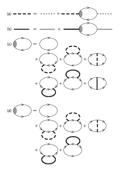
Fig.  1: Diagrammatic representation of the present theory. Solid lines denote electronic Green function while thick (thin) long- and short-dashed lines are renormalized (unrenormalized) AFM and $d$SC fluctuations. The diagrams (a) and (b) represent the Dyson equations for the AFM and $d$SC fluctuations, respectively. The diagrams (c) and (d) are the self-energies for AFM and $d$SC fluctuations. We have kept terms up to the one-loop order in the perturbation expansion of them.

In the usual spin flucutation theories, diagrams containing $d$SC fluctuations are absent. Here we consider the both AFM and dSC fluctuations to understand their interplay. There exists some previous attempts related to this line of approach. For example, the coupling of spins to pairing fluctuations was discussed in the calculation of the uniform spin susceptibility near the superconducting transition .${}^{\hbox{\immediate{\bf{?}})}}$ However this approach did not consider AFM fluctuations. It also did not take an explicit account of electrons around the $(\pi,0)$ point.

The calculated results in fact depend on the choice of the parameter values in the effective action Eq. (2.6). Among other parameter values in (2.6)-(2.13), only those representing the bare distance from the critical point, $\xi^{{}^{(0)}}_{\sigma}{}^{-2}$ and $\xi^{{}^{(0)}}_{d}{}^{-2}$ behave singularly at $T=0$ even for finite values of $\mu$, and they are still most divergent with logarithmic accuracy. Then they crucially determine the qualitative aspects through the dependence on the choices of $t^{\prime}$, $\mu$ and $T$.

Consequently, the role of the self-consistent renormalization procedure is reduced to the determination of $\xi_{\sigma}$ and $\xi_{d}$ from

$$\xi_{\sigma}^{-2} = \xi^{{}^{(0)}}_{\sigma}{}^{-2}+\!\int_{0}^{2E_{c}}\!\frac{d\omega}{\pi}\!\int\!\!\frac{d^{2}{\mbox{\boldmath$k$}}}{(2\pi)^{2}}\coth\frac{\omega}{2T}\left[u_{\sigma\sigma}{\rm Im}\chi_{\sigma}(\omega,{\mbox{\boldmath$k$}})+u_{\sigma d}{\rm Im}\chi_{d}(\omega,{\mbox{\boldmath$k$}})\right]$$ (3.1)

$$\xi_{d}^{-2} = \xi^{{}^{(0)}}_{d}{}^{-2}+\!\int_{0}^{2E_{c}}\!\frac{d\omega}{\pi}\!\int\!\!\frac{d^{2}{\mbox{\boldmath$k$}}}{(2\pi)^{2}}\coth\frac{\omega}{2T}\left[u_{\sigma d}{\rm Im}\chi_{\sigma}(\omega,{\mbox{\boldmath$k$}})+u_{dd}{\rm Im}\chi_{d}(\omega,{\mbox{\boldmath$k$}})\right].$$ (3.2)

Our main results obtained numerically will be discussed in the following section. Here, we comment on the characteristics of the present SCR theory for the mode-mode couplings. First, as in the SCR theory of spin fluctuations in 2D, the system can be ordered only at $T=0$. It agrees with the Mermin-Wagner theorem ${}^{\hbox{\immediate{\bf{?}})}}$ for the AFM order. For the $d$SC, the K-T transition at nonzero temperatures is not possible in our formalism in contrast with what should be. This implies that the treatment of the gauge fluctuations in the SCR theory is inadequate for the description of the K-T transition at $T_{KT}$. However, once all the higher energy degrees of freedom are integrated out, the renormalized superfluid stiffness determines the temperature scale where the pairing correlation length starts growing strongly. Since $T_{KT}$ is of the order of the stiffness according to the K-T theory ,${}^{\hbox{\immediate{\bf{?}})}}$ $T_{KT}$ should occur close to this crossover temperature $T_{\ast}$ in our theory, below which the spin correlation length starts decreasing. In our analysis, we take this temperature scale as the signature of the K-T transition.

Another important point is that though the Gaussian approximation for the electrons around the $(\pi,0)$ point predicts the coexistence of the AFM and the $d$SC, as discussed in § 2, as well as mean-field arguments ,${}^{\hbox{\immediate{\bf{?}})}}$ the inclusion of vertex corrections due to the coupling between AFM and $d$SC modes makes their coexistence difficult. It is simpliy because the coupling between AFM and $d$SC modes are repulsive for realistic cases. The coexistence appears only at $t^{\prime}\!=\!\mu\!=\!0$. The further conditions for their stability are given by $|\Gamma_{d}|<|\Gamma_{\sigma}|u_{\sigma d}/u_{\sigma\sigma}$ and $|\Gamma_{\sigma}|>|\Gamma_{d}|u_{\sigma d}/u_{dd}$ for the AFM, and $|\Gamma_{d}|>|\Gamma_{\sigma}|u_{\sigma d}/u_{\sigma\sigma}$ and $|\Gamma_{\sigma}|<|\Gamma_{d}|u_{\sigma d}/u_{dd}$ for the $d$SC, as shown in Appendix 7. A quite different type of coexistence of dSC and AFM may in principle be possible if different portion of the Fermi surface than $(\pi,0)$ and $(0,\pi)$ contributes to the AFM order while $d$SC order is realized only through contributions around $(\pi,0)$ part. Since we do not seriously treat contributions from $(\pi/2,\pi/2)$ part, this possibility is beyond the scope of this paper.

In what follows, we concentrate on the cases where the $d$SC ground state is realized at $T=0$ while substantial AFM fluctuations also persist. In our analyses, we take $\Gamma_{d}\!=\!\Gamma_{\sigma}$. Then the system shows the competing fluctuations of the AFM and the $d$SC in the normal metallic (but not necessarily Fermi-liquid-like) phase below the mean-field transition temperature.

4 Results

Before showing results, we discuss how the phenomenological parameters are determined. For comparison with experiments of hole-doped high-$T_{c}$ cuprates shown below, we take the following rough estimates; $t=0.25$eV from photoemission data of YBa₂Cu₃O_7-x ,${}^{\hbox{\immediate{\bf{?}},\penalty 1000\hskip 0.91003pt plus 0.70004pt minus 0.70004pt{\bf{?}})}}$ $E_{c}=t$, $c_{\sigma}=0.5t$ and $\gamma^{\!{}^{(0)}}_{\sigma}=t$. Hereafter we take the lattice spacing as the length scale and $t$ as the energy unit. Above choices of $\gamma^{\!{}^{(0)}}_{\sigma}$ and $c_{\sigma}$ are taken similar to those obtained by fitting experimental data of $1/T_{1}T$ and $T_{2G}$ of YBa₂Cu₃O_7-x at high temperatures with the staggered susceptibility of the form (2.12). ${}^{\hbox{\immediate{\bf{?}})}}$ At the moment, some uncertainty exists in determining the parameter values describing $d$SC fluctuations. For simplicity and definiteness, we take $c_{d}=c_{d}$ and $\gamma^{\!{}^{(0)}}_{d}=\gamma^{\!{}^{(0)}}_{\sigma}$. We assume that $t^{\prime}$ and $\mu$ are small compared with those obtained by tight-binding band fittings ${}^{\hbox{\immediate{?})}}$ with the photoemission results ,${}^{\hbox{\immediate{\bf{?}})}}$ and take comparable values to $T_{c}$, so that contributions from the flat shoal regions are dominant. We note that experimentally observed Fermi surface may be reproduced by such parameters due to the strong correlation effects .${}^{\hbox{\immediate{\bf{?}})}}$ For $\xi^{{}^{(0)}}_{\sigma,d}$, we adopt the one-loop results (2.14) and (2.15) with proportionality constants determined so that the spin and pairing correlation lengths at $T=1$ are a unity. Further we take the values of fermionic vertices $\Gamma_{\sigma}=\Gamma_{d}$ which predict $T^{{}^{(0)}}_{N}$ of order of the temperature below which the system enters a critical region. Unfortunately, it is rather difficult to reliably estimate the renormalized values of the mode-mode couplings in the available framework. In this paper, we leave $\Gamma_{\sigma}=\Gamma_{d}$ and the mode-mode couplings as adjustable parameters and pose a question whether the experimental results can be totally reproduced within reasonable choices of their values. Particularly, the following conditions have to be satisfied at least to make more detailed comparisons with the experimental data: First, the onset temperature $T_{\ast}$ where correlation length $\xi_{d}$ starts increasing rapidly should be close to $T_{c}$ in real materials. Second, $\xi_{\sigma}$ at $T=T_{\ast}$ is similar to that obtained in the experiments in each case. Third, the crossover temperature $T_{PG}$ obtained in the case $\varphi=1$ at which $1/T_{1}T$ starts decreasing gives a pseudogap temperature obtained experimentally.

Fig.  2: The calculated spin correlation lengths (solid lines), $1/T_{1}T$ (dashed lines) normalized by its value at $T=1$, $d$SC correlation lengths (long-dashed lines), We have taken $|\Gamma_{\sigma}|=|\Gamma_{d}|=0.15$, $u_{\sigma\sigma}=2.6$, $u_{\sigma d}=1.2$, $u_{dd}=1.8$, $\mu=0.03$ and $t^{\prime}=-0.03$, which correspond to YBa₂Cu₃O₇.

First, for the case $\varphi=0$, we show the case where the parameter values correspond to YBa₂Cu₃O₇ .${}^{\hbox{\immediate{?})}}$ We plot the calculated $d$SC correlation length $\xi_{d}$, $1/T_{1}T$ and spin correlation length $\xi_{\sigma}$ in Fig. 2. As previously mentioned, on this level of approximations, the nature of the original Fermi surface determines whether the ground state is AFM or $d$SC, through the bare irreducible particle-hole and particle-particle susceptibilities. For finite values of $t^{\prime}$ or $\mu$, the ground state is $d$SC in the one-loop results. In this case, the spin correlation length first increases down to the temperature $T_{\ast}$ and then decreases with further decrease in temperature. The crossover temperature $T_{\ast}$ depends on $t^{\prime}$, mode-mode couplings and other parameters in the effective action. It makes a crossover between the regime $T<T_{\ast}$ dominated by the $d$SC renormalized classical fluctuations and the thermally fluctuating regime $T>T_{\ast}$.

The spin-lattice relaxation rate $T_{1}$ of a ⁶³Cu nuclei, after a proper subtraction of the contribution from the uniform part, is evaluated approximately as

$$1/T_{1}T \propto \lim_{\omega\to 0}\!\int\!\!d{\mbox{\boldmath$k$}}{\rm Im}\chi_{\sigma}(\omega,{\mbox{\boldmath$k$}})/\omega$$ (4.1)

$$\propto \xi_{\sigma}^{2}\gamma_{\sigma}/c_{\sigma}^{2}.$$

Here we have not considered the ${\bf k}$-dependence of the nuclear form factor seriously, because it does not alter the basic feature. From (4.1), we see that $1/T_{1}T$ has basically the same temperature dependence as $\xi_{\sigma}^{2}$. By taking $T_{c}$ comparable to $T_{\ast}$, our present result for $\varphi=0$ suggests that overdoped cuprates which show $T_{PG}\sim T_{\ast}\sim T_{c}$ as in Tl₂Ba₂CuO₆, or HgBa₂CuO_4+δ ${}^{\hbox{\immediate{\bf{?}})}}$ are also classified as this class, besides optimally doped systems such as YBa₂Cu₃O₇ .${}^{\hbox{\immediate{?})}}$ We conclude that our calculated results with $\varphi=0$ are totally consistent with the experimental results of optimally as well as overdoped cuprates. Even in the underdoped region, La_2-xSr_xCuO₄ ${}^{\hbox{\immediate{\bf{?}})}}$ seems to belong to this category. Recent ARPES data of La_2-xSr_xCuO₄ clarified exceptionally strong damping in the region $(\pm\pi/2,\pm\pi/2)$. ${}^{\hbox{\immediate{\bf{?}})}}$ This may well be reproduced by $\varphi=0$ class. The absence of clear pseudo gap in the magnetic response in this compound is consistent with this interpretation.

Next we consider $\varphi>0$ cases. Contrary to the case $\varphi=0$, one has to be careful in determining the scaling form of the damping rates. If only AFM spin fluctuations exist, it can follow the simple scaling form $\gamma_{\sigma}\propto\xi_{\sigma}^{-\varphi}$. When we take $\varphi=1$, the $z=1$ scaling holds within the tree level. However, when we treat complicated fluctuations containing both AFM and $d$SC characters tightly coupled each other through $S_{\sigma d}^{(4)}$, the correct theory should involve two different scales $\xi_{\sigma}$ and $\xi_{d}$. Here, note that the lower energy scale (or longer length scale) always determines the damping rates of the modes: physically, the strongest fluctuations affect the fermionic low-energy spectral weights, which dominate the mode dampings. To take into account this feedback effect on the mode dampings, we introduce the following phenomenological relation:

$$\gamma_{\sigma,d}=2\gamma^{\!{}^{(0)}}_{\sigma,d}/(\xi_{\sigma}^{\varphi}+\xi_{d}^{\varphi}).$$ (4.2)

In terms of bosonic excitations, the relaxation times of collective modes should be determined by the time necessary to propagate the scale of the longest correlation length, because the damping is not effective as far as the excitations are propagating inside such an ordered domain. Thus we take $\varphi=1$ here.

Fig.  3: The results for the spin correlation lengths (solid lines), $1/T_{1}T$ (dashed lines), and the $d$SC correlation lengths (long-dashed lines) in the $\varphi=1$ case. We have taken $|\Gamma_{\sigma}|=|\Gamma_{d}|=0.7$, $u_{\sigma\sigma}=3.14$, $u_{dd}=3.05$, $u_{\sigma d}=1.0$, $\mu=0.02$ and $t^{\prime}=-0.02$, which correspond to YBa₂Cu₃O_6.63. As in Fig. 2, the data of $1/T_{1}T$ are normalized by its value at $T=1$.

The calculated $\xi_{\sigma}$, $\xi_{d}$ and $1/T_{1}T$ are shown in Fig. 3 for the parameter values corresponding to YBa₂Cu₃O_6.63. As in $\varphi=0$ cases, with the decrease in temperature, the spin correlation length first increases, reaches its maximum value and then decreases due to the quantum fluctutaions introduced by the renormalized-classical $d$SC fluctuations. This temperature, which we refer to as $T_{\ast}$, is mainly determined from $t^{\prime}$ and the mode-mode coupling constants. On the other hand, $1/T_{1}T$ behaves in a different manner from $\varphi=0$ cases. When the temperature is lowered, $\xi_{\sigma}$ and $\xi_{d}$ both first gradually increase. In this region, $1/T_{1}T$ also gradually increases. With further decrease in temperature, $\xi_{d}$ starts growing quicker than $\xi_{\sigma}$ and then $\gamma_{\sigma}$ starts decreasing much quicker than $\xi_{\sigma}$ at $T_{PG}$. This drives spin excitations from overdamped into underdamped region, and forms a spin-excitation peak at a finite frequency $\omega=\omega^{*}$ in $S(Q,\omega)$. Namely, the spectral weight start transferring from $\omega=0$ to the peak region around $\omega^{*}$, which makes decrease in $1/T_{1}T$. A similar crossover was previously obtained in a numerical calculation near the quantum transition point between $d$SC and AFM ordered phases .${}^{\hbox{\immediate{\bf{?}},\penalty 1000\hskip 0.91003pt plus 0.70004pt minus 0.70004pt{\bf{?}},\penalty 1000\hskip 0.91003pt plus 0.70004pt minus 0.70004pt{\bf{?}})}}$ At lower temperatures characterized by $T_{\ast}$, the $d$SC fluctuations go into the renormalized classical regime, which signals the decrease in $\xi_{\sigma}$. We again interpret $T_{\ast}$ as the rough estimate of $T_{c}$. These properties are also similar to experimental data in underdoped cuprates with a pseudo spin gap, such as YBa₂Cu₄O₈ ${}^{\hbox{\immediate{?})}}$ and Bi₂Sr₂Ca₁Cu₂O₈ .${}^{\hbox{\immediate{?})}}$ In the present framework, the crossover $T_{PG}$ increases with increasing $t^{\prime}$, because it accelerates the dominance of $d$SC correlations over AFM, which induces reduction of $\gamma_{\sigma}$. Figure 4 indeed shows that $T_{PG}$ increases with $t^{\prime}$. Figure 5 shows the calculated results for $\varphi=1$ and $\mu=t^{\prime}=0$ with $u_{\sigma\sigma}$ less than $u_{dd}$, so that $\xi_{\sigma}$ shows a stronger divergence than $\xi_{d}$ and the ground state is very close to the quantum transition point between AFM and $d$SC.

Fig.  4: Spin correlation lengths (solid lines) and $1/T_{1}T$ (dashed lines) calculated in the case of $\varphi=1$ for $|t^{\prime}|=0.02$, $0.06$ and $0.1$ from top to bottom curves, and $d$SC correlation lengths (long-dashed lines) from bottom to top curves. We have taken $|\Gamma_{\sigma}|=|\Gamma_{d}|=0.7$, $u_{\sigma\sigma}=3.14$, $u_{dd}=3.05$, $u_{\sigma d}=1.0$, $\mu=0.02$. It suggests that as $|t^{\prime}|$ become larger, $T_{\ast}$ and $T_{PG}$ increase.

Fig.  5: The results for the spin correlation lengths (solid lines), $1/T_{1}T$ (dashed lines), and the $d$SC correlation lengths (long-dashed lines) in the $\varphi=1$ case. We have taken $|\Gamma_{\sigma}|=|\Gamma_{d}|=0.7$, $u_{\sigma\sigma}=3.0$, $u_{dd}=3.1$, $u_{\sigma d}=1.0$, $\mu=0$ and $t^{\prime}=0$, so that the spin correlation length shows a stronger divergence than the $d$SC correlation length.

Irrespective of the damping rate exponent $\varphi$, low-energy spin fluctuations are in general suppressed due to the $d$SC fluctuations around its ordered state. However, the manner of suppression is different between $\varphi=0$ and $1$, i.e., between the case that low-energy fermions coupled to collective modes exist and the case that those are absent.

The peak structure in $S(Q,\omega)$ around $\omega^{*}$ reproduces some qualitative feature in the resonance peak observed experimentally .${}^{\hbox{\immediate{?},\penalty 1000\hskip 0.91003pt plus 0.70004pt minus 0.70004pt{\bf{?}})}}$ In our treatment, $\omega^{*}$ is selfconsistently determined from the competition between $d$SC and AFM and the value $\omega^{*}$ is characterized by the $d$SC gap amplitude. The AFM fluctuations are pushed out from the region lower than $\omega^{*}$ due to the dSC pseudogap formation.

Experimentally, the resonance peak appears to be sharpened with the increasing $d$SC correlation length $\xi_{d}$ and the intensity of the peak remarkably increases below the superconducting $T_{c}$. This implies a rapid growth of the AFM correlation length $\xi_{\sigma}$. On the other hand, $\omega^{*}$ does not strongly depend on the temperature. The frequency $\omega^{*}$ depends only on the doping concentration. It in fact decreases only when the doping concentration is decreased. A similar feature is also seen numerically near the AFM-$d$SC transition .${}^{\hbox{\immediate{?},\penalty 1000\hskip 0.91003pt plus 0.70004pt minus 0.70004pt{?})}}$ This feature is beyond the scope of this paper, because, in our framework of (2.12), $\omega^{\ast}$ has to be proportional to $\xi_{\sigma}^{-1}$ for small $\gamma_{\sigma}$. To realize rapidly increasing correlation length with a fixed finite $\omega^{\ast}$, we need to modify the assumed form (2.12) as discussed before .${}^{\hbox{\immediate{?})}}$ To reproduce the temperature dependence, it will be necessary to correctly take into account dominat incoherent part in addition to the coherent response, although our susceptibility (2.12) overlooks such a subtlety.

5 Conclusion

The pseudogap region observed in the high-$T_{c}$ is reproduced as the region with enhanced $d$SC correlations. The experimental results for the magnetic excitations are consistently explained from precursor effects for the superconductivity.

From the electrons around the flat spots, $(\pi,0)$ and $(0,\pi)$, we have considered the low-energy effective action for the auxilary fields for the AFM and $d$SC. The one-particle irreducible vertices for both channels have been taken negative values, as suggested by one-loop renormalization group studies .${}^{\hbox{\immediate{?},\penalty 1000\hskip 0.91003pt plus 0.70004pt minus 0.70004pt{?},\penalty 1000\hskip 0.91003pt plus 0.70004pt minus 0.70004pt{?})}}$ Next, we have obtained solutions of the self-consistent one-loop renormalization. The inclusion of vertex correction in 2D suppresses finite-temperature transitions. This correctly reproduces the absence of antiferromagnetic transition at nonzero $T$ in 2D. The superconducting Kosterlitz-Thouless-Berezinski transition is also absent in this approximation in contrast to what should be. This is just an artifact due to neglect of the phase modes of the $d$SC order parameter. In this paper, we take $T_{\ast}$ as a rough estimate of $T_{c}$, where $T_{\ast}$ is defined as the onset temperature for the renormalized classical regime of the $d$-wave pairing. Below this temperature, spin correlation length starts decreasing. Because of the repulsive coupling between $d$SC and AFM modes, the coexistence of the $d$SC and the AFM orders does not take place except when both degrees of freedom are nearly symmetric as explained in Appendix 7.

The pseudogap formation clarified from the interplay of AFM and $d$SC is summarized as follows: When either the Fermi level $\mu$ measured from the flat spot or the next nearest-neighbor hopping $t^{\prime}$ is nonzero, the $d$SC ground state is realized. Only in a special case of $\mu=t^{\prime}=0$, $d$SC, AFM or coexistent ground state can be realized depending on the values of the mode-mode couplings as discussed in Appendix 7. When the $d$SC correlation grows faster, the process of the pseudogap formation depends on the damping exponent $\varphi$. If $\varphi=0$, namely the damping $\gamma$ does not depend on the $d$SC correlation length, the spin correlation length, $\xi_{\sigma}$ and $1/({}^{63}T_{1}T)$ both reaches its maximum value at $T=T_{\ast}$ and then decreases as the temperature decreases. On the other hand, when the mode dampings are suppressed near the transition, e.g., $\varphi=1$, $1/(T_{1}T)$ shows a faster decrease at $T_{PG}(>T_{\ast})$ while $\xi_{\sigma}$ continues to increase until $T_{\ast}$. The pseudogap temperature $T_{PG}$ increases as $t^{\prime}$ increases and it tends to decrease when the nesting effect of the Fermi surface around the flat spot becomes stronger.

In comparison with experiments in the cuprates, the results for $\varphi=0$ reproduce the feature obtained in the optimally doped and overdoped high-$T_{c}$ cuprates, such as YBa₂Cu₃O₇ ${}^{\hbox{\immediate{?})}}$ and Tl₂Ba₂CuO₆ and HgBa₂CuO_4+δ ,${}^{\hbox{\immediate{?})}}$ and even some underdoped cases as La_2-xSr_xCuO₄ .${}^{\hbox{\immediate{?})}}$ For this category, we speculate that quasi-particle excitations around $(\pi/2,\pi/2)$ point mainly contribute to the finite damping of AFM fluctuations.

On the other hand, in many underdoped high-$T_{c}$ cuprates, $1/(T_{1}T)$ starts decreasing at $T_{PG}$ above $T_{c}$, while the spin correlation length measured by $T_{2G}$ shows the Curie-Weiss behavior down to $T_{c}$ .${}^{\hbox{\immediate{?},\penalty 1000\hskip 0.91003pt plus 0.70004pt minus 0.70004pt{?},\penalty 1000\hskip 0.91003pt plus 0.70004pt minus 0.70004pt{?},\penalty 1000\hskip 0.91003pt plus 0.70004pt minus 0.70004pt{?})}}$ This pseudogap behavior is reproduced by our $\varphi=1$ case, if we take $T_{\ast}$ as the superconducting transition temperature. In addition, the qualitative similarity between our results for $\varphi=1$ and the experimental results suggests that the damping of the AFM and $d$SC collective modes decreases in the pseudogap regime. It means that low-energy fermions around the flat spots mainly contribute to the damping. This is consistent with the strong damping of quasiparticle around the flat spot observed experimentally in the underdoped region. This flat dispersion is a consequence of the universal character of the metal-insulator transition.

We clearly need further studies for a more complete understanding of the pseudogap in the high-$T_{c}$ cuprates. After the present work, several important steps still remain. In the next step from the present work, a more systematic renormalization group treatment would be interesting .${}^{\hbox{\immediate{\bf{?}})}}$ We have concentrated on the single-particle excitations only around the flat spots, $(\pi,0)$ and $(0,\pi)$ assuming their crucial importance in the mechanism of the pseudogap formation. However, in the one-loop level, the origin of the flat dispersion and strong damping in this momentum region is not fully understood. Experimentally the flatness and damping strength appear much more pronounced than the expectation from the one-loop analyses. Numerical analyses also support that this remarkable momentum dependence around the flat spots is due to strong correlation effects. We have to calculate self-energy corrections as well as the vertex corrections in a selfconsistent fashion to clarify the profoundness of such correlation effects. This is clearly the step beyond the one-loop level. Near the metal-insulator transition point, vanishing quasiparticle weight has to be led from a selfconsistent treatment. This will contribute to clarify how the pairing channel appears and how the flat spots are destabilized to the paired singlet. We also note that the dominance of the incoherent weight over the quasiparticle weight in the single-particle excitations near the metal-insulator transition may require a serious modification in the derivation of the AFM and $d$SC susceptibilities. The Curie-Weiss type form for the dynamic spin susceptibility needs to be reconsidered  ,${}^{\hbox{\immediate{?})}}$ because the spin susceptibility is also determined mainly from the incoherent part of the single-particle excitations which we have not considered at all in this paper. In addition, we have not considered effects of quasiparticles excitated far from the flat spots. In this context, a more comprehensive analyses are required to see the momentum dependence.

6 Calculation of the coupling constants

Here we give the quartic coupling constants at the lowest energy and the wave vector measured from the ordering one. If we take $g({\mbox{\boldmath$k$}})={\rm sgn}(\cos k_{x}-\cos k_{y})$, after straightforward calculations one obtains

$$u_{\sigma\sigma} = \frac{\Gamma_{\sigma}^{2}}{2(2\pi)^{4}}T^{3}\sum_{m}\!\int\!\!d^{2}{\mbox{\boldmath$k$}}G(i\Omega_{m},{\mbox{\boldmath$k$}})^{2}G(i\Omega_{m},{\mbox{\boldmath$k$}}-{\mbox{\boldmath$Q$}})^{2}$$ (6.1)

$$= \frac{\Gamma_{\sigma}^{2}}{2(2\pi)^{4}}T^{2}\!\int\!\!d^{2}{\mbox{\boldmath$k$}}\frac{1}{(\varepsilon_{\mbox{\boldmath$k$}}-\varepsilon_{{\mbox{\boldmath$k$}}-{\mbox{\boldmath$Q$}}})^{2}}{\hbox{$\left[\vbox to0.0pt{}\right.\n@space$}}\frac{\tanh\varepsilon_{\mbox{\boldmath$k$}}/2T-\tanh\varepsilon_{{\mbox{\boldmath$k$}}-{\mbox{\boldmath$Q$}}}}{\varepsilon_{\mbox{\boldmath$k$}}-\varepsilon_{{\mbox{\boldmath$k$}}-{\mbox{\boldmath$Q$}}}}-\frac{1}{2T}{\rm sech}^{2}\varepsilon_{\mbox{\boldmath$k$}}/2T{\hbox{$\left]\vbox to0.0pt{}\right.\n@space$}}$$ (6.2)

$$u_{dd} = \frac{\Gamma_{d}^{2}}{2(2\pi)^{4}}T^{3}\sum_{m}\!\int\!\!d^{2}{\mbox{\boldmath$k$}}G(i\Omega_{m},{\mbox{\boldmath$k$}})^{2}G(-i\Omega_{m},-{\mbox{\boldmath$k$}})^{2}$$ (6.3)

$$= \frac{\Gamma_{d}^{2}}{8(2\pi)^{4}}T^{2}\!\int\!\!d^{2}{\mbox{\boldmath$k$}}\varepsilon_{\mbox{\boldmath$k$}}^{-2}{\hbox{$\left[\vbox to0.0pt{}\right.\n@space$}}\varepsilon_{\mbox{\boldmath$k$}}^{-1}\tanh\varepsilon_{\mbox{\boldmath$k$}}/2T-\frac{1}{2T}{\rm sech}^{2}\varepsilon_{\mbox{\boldmath$k$}}/2T{\hbox{$\left]\vbox to0.0pt{}\right.\n@space$}}$$ (6.4)

$$u_{\sigma d} = -\frac{\Gamma_{\sigma}\Gamma_{d}}{2(2\pi)^{4}}T^{3}\sum_{m}\!\int\!\!d^{2}{\mbox{\boldmath$k$}}G(i\Omega_{m},{\mbox{\boldmath$k$}})G(-i\Omega_{m},-{\mbox{\boldmath$k$}})$$ (6.6)

$$\left\{G(i\Omega_{m},{\mbox{\boldmath$k$}}-{\mbox{\boldmath$Q$}})G(-i\Omega_{m},-{\mbox{\boldmath$k$}})-G(\Omega_{m},{\mbox{\boldmath$k$}}-{\mbox{\boldmath$Q$}})G(-i\Omega_{m},-{\mbox{\boldmath$k$}}+{\mbox{\boldmath$Q$}})\right\}$$

$$= \frac{\Gamma_{\sigma}\Gamma_{d}}{8(2\pi)^{4}}T^{2}\!\int\!\!d^{2}{\mbox{\boldmath$k$}}{\hbox{$\left[\vbox to0.0pt{}\right.\n@space$}}-\frac{\varepsilon_{\mbox{\boldmath$k$}}^{-1}\tanh\varepsilon_{\mbox{\boldmath$k$}}/2T-\varepsilon_{\mbox{\boldmath$k$}-Q}^{-1}\tanh\varepsilon_{{\mbox{\boldmath$k$}}-{\mbox{\boldmath$Q$}}}/2T}{\varepsilon_{\mbox{\boldmath$k$}}^{2}-\varepsilon_{{\mbox{\boldmath$k$}}-{\mbox{\boldmath$Q$}}}^{2}}$$

$$-\frac{1}{\varepsilon_{\mbox{\boldmath$k$}}+\varepsilon_{{\mbox{\boldmath$k$}}-{\mbox{\boldmath$Q$}}}}{\hbox{$\left(\vbox to0.0pt{}\right.\n@space$}}\varepsilon_{\mbox{\boldmath$k$}}^{-2}\tanh\varepsilon_{\mbox{\boldmath$k$}}/2T-\frac{\varepsilon_{\mbox{\boldmath$k$}}^{-1}}{2T}{\rm sech}^{2}\varepsilon_{\mbox{\boldmath$k$}}/2T{\hbox{$\left)\vbox to0.0pt{}\right.\n@space$}}{\hbox{$\left]\vbox to0.0pt{}\right.\n@space$}}.$$

$u_{\sigma\sigma}$ and $u_{dd}$ are always positive. $u_{\sigma d}$ is positive when $0\leq-\mu<t+2t^{\prime}$, $0\leq\mu<t-2t^{\prime}$, or $T>|\mu|$ holds approximately. Otherwise it is negative. Consequently, it is positive for typical Fermi surface of high-$T_{c}$ cuprates. They are finite at least at finite temperatures, thus, at the energy cutoff.

7 Phase diagram at $T=0$ for nested cases

In this appendix, we discuss what type of ground states is established in the presence of positive $u_{\sigma d}$. We, however, regard that $u_{\sigma d}$ is small enough so that $u_{\sigma\sigma}u_{dd}>u_{\sigma d}^{2}$.

To find the lowest excitation spectrum, it is convenient to rewrite (3.1) and (3.2) in the following expressions,

$$\xi_{\sigma}^{-2} = \xi^{{}^{(0)}}_{\sigma}{}^{-2}+\frac{u_{\sigma d}}{u_{dd}}(\xi_{d}^{-2}-\xi^{{}^{(0)}}_{d}{}^{-2})+(u_{\sigma\sigma}-\frac{u_{\sigma d}^{2}}{u_{dd}})\!\int_{0}^{2E_{c}}\!\frac{d\omega}{\pi}\!\int\!\frac{d^{2}{\mbox{\boldmath$k$}}}{(2\pi)^{2}}{\rm Im}\chi_{\sigma}(\omega,{\mbox{\boldmath$k$}})\coth\frac{\omega}{2T}$$ (7.1)

$$\xi_{d}^{-2} = \xi^{{}^{(0)}}_{d}{}^{-2}+\frac{u_{\sigma d}}{u_{\sigma\sigma}}(\xi_{\sigma}^{-2}-\xi^{{}^{(0)}}_{\sigma}{}^{-2})+(u_{dd}-\frac{u_{\sigma d}^{2}}{u_{\sigma\sigma}})\!\int_{0}^{2E_{c}}\!\frac{d\omega}{\pi}\!\int\!\!\frac{d^{2}{\mbox{\boldmath$k$}}}{(2\pi)^{2}}{\rm Im}\chi_{d}(\omega,{\mbox{\boldmath$k$}})\coth\frac{\omega}{2T}.$$ (7.2)

When $t^{\prime}\neq 0$ or $\mu\neq 0$, within weak coupling arguments (2.14) and (2.15), $d$SC ordered state is realized at $T=0$. It is because at sufficiently low temperatures, $\xi^{{}^{(0)}}_{\sigma}{}^{-2}+(\xi_{d}^{-2}-\xi^{{}^{(0)}}_{d}{}^{-2})u_{\sigma d}/u_{dd}$ becomes positive, while $\xi^{{}^{(0)}}_{d}{}^{-2}+(\xi_{\sigma}^{-2}-\xi^{{}^{(0)}}_{\sigma}{}^{-2})u_{\sigma d}/u_{\sigma\sigma}$ has a large negative value. For the nested case, $\mu=t^{\prime}=0$, the insertion of (2.14) and (2.15) into (7.1) and (7.2) lead to the followings;

$$\xi_{\sigma}^{-2} \!= \!-(\Gamma_{\sigma}-\frac{u_{\sigma d}}{u_{dd}}\Gamma_{d})/t\log^{2}\frac{E_{c}}{T}+\xi_{d}^{-2}u_{\sigma d}/u_{dd}+(u_{\sigma\sigma}-\frac{u_{\sigma d}^{2}}{u_{dd}})\!\int_{0}^{2E_{c}}\!\!\frac{d\omega}{\pi}\!\int\!\!\frac{d^{2}{\mbox{\boldmath$k$}}}{(2\pi)^{2}}{\rm Im}\chi_{\sigma}(\omega,{\mbox{\boldmath$k$}})\coth\frac{\omega}{2T}$$ (7.3)

$$\xi_{d}^{-2} \!= \!-(\Gamma_{d}-\frac{u_{\sigma d}}{u_{\sigma\sigma}}\Gamma_{\sigma})/t\log^{2}\frac{E_{c}}{T}+\xi_{\sigma}^{-2}u_{\sigma d}/u_{\sigma\sigma}+(u_{dd}-\frac{u_{\sigma d}^{2}}{u_{\sigma\sigma}})\!\int_{0}^{2E_{c}}\!\!\frac{d\omega}{\pi}\!\int\!\!\frac{d^{2}{\mbox{\boldmath$k$}}}{(2\pi)^{2}}{\rm Im}\chi_{d}(\omega,{\mbox{\boldmath$k$}})\coth\frac{\omega}{2T}.$$ (7.4)

at sufficiently low temperatures. Therefore ground state properties are determined by $\Gamma_{\sigma}-\Gamma_{d}u_{\sigma d}/u_{dd}$ and $\Gamma_{d}-\Gamma_{\sigma}u_{\sigma d}/u_{\sigma\sigma}$. If the former is positive and the latter is negative, the system has the AFM order. If the former is negative and the latter is positive, it has the $d$SC order. If both values are positive, both orders may coexist and thus $\pi$-triplet fluctuations are also required to consider. If both values are negative, it belongs to the quantum-disordered region.

References

- [1] For a recent review see M. Imada, A. Fujimori and Y. Tokura: Rev. Mod. Phys. 70 (1998) 1039, Sec IV.C.
- [2] Z. -X. Shen and D. S. Dessau: Physics Reports 253 (1995) 1; A. G. Loesser et al.: Science 273 (1996) 325.
- [3] H. Ding et al.: Nature 382 (1996) 51; D. S. Marshall et al.: Phys. Rev. Lett. 76 (1996) 4841.
- [4] M. Imada, F. F. Assaad, H. Tsunetsugu and Y. Motome: cond-mat/9808044 and to be published.
- [5] F. F. Assaad and M. Imada: cond-mat/9811384.
- [6] For a recent review see M. Imada, A. Fujimori and Y. Tokura: Rev. Mod. Phys. 70 (1998) 1039, Sec II.F.11.
- [7] H. Yasuoka, T. Imai and T. Shimizu: “Strong Correlation and Superconductivity” ed. by H. Fukuyama, S. Maekawa and A. P. Malozemoff (Springer Verlag, Berlin, 1989), p.254.
- [8] H. Zimmermann, M. Mali, D.Brinkmann, J. Karpinski, E. Kaldis and S. Rusiecki: Physica C 159 (1989) 681; T. Machi, I. Tomeno, T. Miyataka, N. Koshizuka, S. Tanaka, T. Imai and H. Yasuoka: Physica C 173 (1991) 32.
- [9] K. Ishida, Y. Kitaoka, K. Asayama, K. Kadowaki and T. Mochiku: Physica C 263 (1996) 371.
- [10] Y. Itoh, T. Machi, A. Fukuoka, K. Tanabe, and H. Yasuoka: J. Phys. Soc. Jpn. 65 (1996) 3751.
- [11] M. -H. Julien et al.: Phys. Rev. Lett. 76 (1996) 4238.
- [12] H. F. Fong, B. Keimer, D. L. Milius and I. A. Aksay: Phys. Rev. Lett. 78 (1997) 713.
- [13] See Ref. Sec.II.D,E,F and IV.C.
- [14] A. J. Leggett: J. Phys. (France) 41 (1980) C7.
- [15] P. Nozière and S. Schmitt-Rink: J. Low. Temp. Phys. 59 (1985) 195.
- [16] V. J. Emery and S. A. Kivelson: Nature 374 (1995) 434.
- [17] M. Randeria: cond-mat/9710223, and references therein.
- [18] B. C. den Hetrog: cond-mat/9808051.
- [19] H. J. Schulz: Europhys. Lett. 4 (1987) 609.
- [20] I. E. Dzyaloshinskii: J. Phys. I (France) 6 (1996) 119.
- [21] N. Furukawa, T. M. Rice and M. Salmhofer: Phys. Rev. Lett. 81 (1998) 3195.
- [22] T. Moriya: Spin Fluctuation in Itenerant Electron Magnetism (Springer-Verlag, Berlin, 1985).
- [23] S. Chakravarty, B. I. Halperin and D. R. Nelson: Phys. Rev. B 39 (1989) 2344.
- [24] A. V. Chubukov, S. Sachdev and J. Ye: Phys. Rev. B 49 (1994) 11919.
- [25] J. A. Hertz and M. A. Klenin: Phys. rev. B 10 (1974) 1084.
- [26] J. A. Hertz: Phys. Rev. B 14 (1976) 1165.
- [27] A. J. Millis: Phys. Rev. B 48 (1993) 7183.
- [28] K. Gofron, J. C. Campuzano, A. A. Abrikosov, M. Lindroos, A. Bansil, H. Ding, D. Koelling and B. Dabrowski: Phys. Rev. Lett. 73 (1994) 3302.
- [29] S. Sachdev, A. V. Chubukov and A. Sokol: Phys. Rev. B 51 (1995) 14874.
- [30] J. Schmalian: cond-mat/9810041.
- [31] S.-C. Zhang: Science 275 (1997) 1089.
- [32] S.-C. Zhang: cond-mat/9808309.
- [33] L. Berezinski: Sov. Phys. JETP 32 (1970) 493; J. M. Kostelitz and D. J. Thouless: J. Phys. C6 (1973) 1181.
- [34] M. Randeria and A. Varlamov: Phys. Rev. B 50 (1994) 10401.
- [35] M. D. Mermin and H. Wagner: Phys. Rev. Lett. 17 (1966) 1133.
- [36] M. Murakami and H. Fukuyama: J. Phys. Soc. Jpn. 67 (1998) 2784.
- [37] S. Massidda, J. Yu and A. J. Freeman: Phys. Lett. A 122 (1987) 198.
- [38] Q. Si, Y. Zha, K. Levin and J. P. Lu: Phys. Rev. B 47 (1993) 9055.
- [39] J. C. Compuzano, et al.: Phys. Rev. Lett. 64 (1990) 2308.
- [40] P. Monthoux and D. Pines: Phys. Rev. B 50 (1994) 16015.
- [41] H. Tsunetsugu and M. Imada: unpublished.
- [42] Y. Itoh, T. Machi, A. Fukuoka, K. Tanabe and H. Yasuoka: J. Phys. Soc. Jpn. 65 (1996) 3751.
- [43] T. Imai et al.: J. Phys. Soc. Jpn. 59 (1990) 3846.
- [44] A. Ino et al.: cond-mat/9809311; Phys. Rev. Lett. 79 (1997) 2101; Phys. Rev. Lett. 80 (1998) 2124.
- [45] F. F. Assaad, M. Imada, and D. J. Scalapino: Phys. Rev. Lett. 77 (1996) 4592.
- [46] F. F. Assaad, M. Imada, and D. J. Scalapino: Phys. Rev. B 56 (1997) 15001.
- [47] F. F. Assaad, and M. Imada: Phys. Rev. B 58 (1998) 1845.
- [48] J. Rossat-Mignod et al.: Physica C 185-189 (1991) 86.
- [49] S. Onoda and M. Imada: unpublished.