Statistical reconstruction of three-dimensional porous media from two-dimensional images

Abstract

A method of modelling the three-dimensional microstructure of random isotropic two-phase materials is proposed. The information required to implement the technique can be obtained from two-dimensional images of the microstructure. The reconstructed models share two-point correlation and chord-distribution functions with the original composite. The method is designed to produce models for computationally and theoretically predicting the effective macroscopic properties of random materials (such as electrical and thermal conductivity, permeability and elastic moduli). To test the method we reconstruct the morphology and predict the conductivity of the well known overlapping sphere model. The results are in very good agreement with data for the original model.

47.55.Mh, 44.30.+v, 81.05.Rm, 61.43.Bn

Predicting the macroscopic properties of composite or porous materials with random microstructures is an important problem in a range of fields [3, 4]. There now exist large-scale computational methods for calculating the properties of composites given a digital representation of their microstructure (eg. permeability [5, 6], conductivity [5, 6, 7] and elastic moduli [8]). A critical problem is actually obtaining an accurate three-dimensional description of this microstructure [5, 9, 10]. For particular materials it may be possible to simulate microstructure formation from first principles. Generally this relies on a detailed knowledge of the physics and chemistry of the system; the accurate modelling of each material requiring a significant amount of research. Where such information is unavailable an alternative is to directly [11, 12, 13, 14, 15, 16, 17] or statistically [5, 6, 10, 18, 19, 20, 21, 22, 23] reconstruct the microstructure from experimental images.

Several techniques of direct reconstruction have been implemented. A composite can be repeatedly sectioned, imaged and the results combined to reproduce a three-dimensional digital image of the microstructure [11, 12, 13]. For porous materials, time consuming sectioning can been avoided by using laser microscopy [14] which can image pores to depths of around 150$\mu$m. Recent micro-tomography studies have also directly imaged the three-dimensional microstructure of porous sandstones [15, 16] and magnetic gels [17]. The complexity and restrictions of these methods provide the impetus to study alternative reconstruction methods.

Based on the work of Joshi [18], Quiblier [19] introduced a method of generating a three-dimensional statistical reconstruction of a random composite. The method is based on matching statistical properties of a three-dimensional model to those of a real microstructure. A key advantage of this approach is that the required information can be obtained from a two dimensional image of the sample. Recently the method has been applied to the reconstruction of sandstone [6, 10, 20, 21] and a material composed of overlapping spheres [5]. Computations of the permeability and conductivity [5, 6, 20] of the reconstructed images underestimate experimental data by around a factor of three. This can be partially attributed to the fact that percolation threshold of the reconstructed models is around 10% while the experimental systems had thresholds of less than 3% [5]. Recent work in microstructure modelling has led to a general scheme [7, 24, 25, 26, 27, 28, 29] (§ I) which includes the model employed by Quiblier. Importantly, other models in the scheme can mimic the low percolation thresholds observed in sandstones (and many other materials [24]). It is therefore timely to reconsider statistical methods of reconstructing composite microstructure.

Prior methods of statistical reconstruction produce three-dimensional models which share first (volume fraction) and second (two-point correlation function) order statistics with the original sample. However the complete statistical description of a random disordered material requires higher order information [10, 30] (eg. the three and four point correlation functions). Information which in turn is a crucial ingredient of rigourous theories of macroscopic properties [3, 30, 31], and therefore important to the success of the model. In this paper we show that reconstructions based on matching first and second order statistics do not necessarily provide good models of the original composite (§ II). An alternative method of reconstruction is proposed and tested (§ III). The procedure is employed to reconstruct a composite generated from identical overlapping spheres (IOS) and successfully predicts the electrical conductivity of the model (§ IV).

I Model composite materials

To study the statistical properties of composites it is conventional to introduce a phase function $\phi(\mbox{\boldmath$r$})$ which equals unity or zero as $r$ is in phase one or two. The volume fraction of phase one is $p=\langle\phi\rangle$, while the standard two-point correlation function is defined as $p^{(2)}(r)=\langle\phi(\mbox{\boldmath$r$}_{1})\phi(\mbox{\boldmath$r$}_{2})\rangle$ with $r$=$|\mbox{\boldmath$r$}_{2}-\mbox{\boldmath$r$}_{1}|$ (assuming the material is statistically homogeneous and isotropic). $p^{(2)}(r)$ represents the probability that two points a distance $r$ apart will lie in phase one. From the definition $p^{(2)}(0)=p$ and $\lim_{r\to\infty}p^{(2)}(r)\to p^{2}$. The surface area per unit volume is $s=-4dp^{(2)}/dr|_{r=0}$ [32]. Higher order functions can be analogously defined, these playing a central role in rigourous theories of composite properties [30]. In practice the correlation functions of real composites beyond second order are difficult to measure and there are significant advantages in developing models for which the functions are exactly known. The primary models in this class are the identical overlapping sphere model (IOS) [33], its generalisation to overlapping annuli [24] and models derived from Gaussian random fields (GRFs) [7, 24, 34, 35] which are central to reconstruction procedures.

We utilise two methods of generating isotropic GRFs. Each has specific advantages which we discuss. The first method develops the random field in a cube of side-length $T$ using a Fourier summation;

$$y(\mbox{\boldmath$r$})=\sum_{l=-N}^{N}\sum_{m=-N}^{N}\sum_{n=-N}^{N}c_{lmn}e^{i\mbox{\boldmath$k$}_{lmn}.\mbox{\boldmath$r$}}$$ (1)

where $\mbox{\boldmath$k$}_{lmn}=\frac{2\pi}{T}(l\mbox{\boldmath$i$}+m\mbox{\boldmath$j$}+n\mbox{\boldmath$k$})$. The statistics of the field are determined by the random variables $c_{l,m,n}$=$a_{lmn}+ib_{lmn}$ ($a_{lmn}$ and $b_{lmn}$ real). We require that $y$ is real ($c_{l,m,n}$=$\bar{c}_{-l,-m,-n}$) and that $\langle y\rangle=0$ ($c_{0,0,0}$=$0$). To ensure isotropy we also take $c_{lmn}$=$0$ for $k_{lmn}$=$|\mbox{\boldmath$k$}_{lmn}|$$\geq$$2\pi N/T$. To generate a Gaussian field the coefficients $a_{lmn}$ are taken as random independent variables (subject to the conditions on $c_{lmn}$) with Gaussian distributions such that $\langle a_{lmn}\rangle=0$ and $\langle a_{lmn}^{2}\rangle$=$\frac{1}{2}\rho(k_{lmn})\left({\frac{2\pi}{T}}\right)^{3}$ (similarly for $b_{lmn}$). The function $\rho(k)$ is a spectral density. It can be shown that a random field defined in this manner has field-field correlation function

$$g(r)\equiv\langle y({\bf r}_{1})y({\bf r}_{2})\rangle=\int_{0}^{\infty}{4\pi k^{2}\rho(k)\frac{\sin kr}{kr}}{dk}.$$ (2)

By convention $g(0)=1$ which sets a constant of proportionality on $\rho(k)$. The definition (1) can be efficiently evaluated by an FFT routine [7] and is $T$-periodic in each direction. This is valuable for approximating an infinite medium in calculations of macroscopic properties.

Alternatively a random field can be generated using the “random-wave” form [36, 34]

$$y(\mbox{\boldmath$r$})=\sqrt{\frac{2}{N}}\sum_{i=1}^{N}\cos(k_{i}\hat{\mbox{\boldmath$k$}}_{i}\cdot{\mbox{\boldmath$r$}}+\phi_{i}),$$ (3)

where $\phi_{i}$ is a uniform deviate on $[0,2\pi)$ and $\hat{\mbox{\boldmath$k$}}_{i}$ is uniformly distributed on a unit sphere. The magnitude of the wave vectors $k_{i}$ are distributed on $[0,\infty)$ with a probability (spectral) density $P(k)$ ($\int_{0}^{\infty}P(k)dk=1$). In terms of the first definition $P(k)=4\pi k^{2}\rho(k)$. In this case the fields are not periodic, but $N$ can be chosen arbitrarily largely over a specified $k$ range. This is especially useful for resolving $\rho(k)$ (so that Eq. (2) holds) in cases where it is strongly spiked (eg. $P(k)=\delta(k)$) [35].

Model composite materials can be defined from a GRF $y({\mbox{\boldmath$r$}})$ by taking the region in space where $\alpha\leq y(\mbox{\boldmath$r$})\leq\beta$ as phase one and the the remaining regions ($y(\mbox{\boldmath$r$})<\alpha$ and $y(\mbox{\boldmath$r$})>\beta$) as phase two. This is the “two-level cut” random field of Berk [36]. In the case $\alpha=-\infty$ the more common “one-level cut” field is recovered [7, 19, 34]. The phase function of this model is $\phi(y(\mbox{\boldmath$r$}))=H(y(\mbox{\boldmath$r$})-\alpha)-H(y(\mbox{\boldmath$r$})-\beta)$ where $H$ is the Heaviside step function. The joint probability distribution of the correlated random variables $\mbox{\boldmath$y$}=[y(\mbox{\boldmath$r$}_{1}),y(\mbox{\boldmath$r$}_{2}),\dots,y(\mbox{\boldmath$r$}_{n})]^{T}$ is, $P_{n}(\mbox{\boldmath$y$})=((2\pi)^{n}|G|)^{-\frac{1}{2}}\exp(-\frac{1}{2}\mbox{\boldmath$y$}^{T}G^{-1}\mbox{\boldmath$y$})$ where the elements of $G$ are $g_{ij}=g(r_{ij})=\langle y({\mathbf{r}}_{i})y({\mathbf{r}}_{j})\rangle$. Therefore the $n$-point correlation function is

$$p^{(n)}=\int_{-\infty}^{\infty}\int_{-\infty}^{\infty}\dots\int_{-\infty}^{\infty}P_{n}(\mbox{\boldmath$y$})\prod_{i=1}^{n}\phi(y(\mbox{\boldmath$r$}_{i}))d\mbox{\boldmath$y$}.$$ (4)

The volume fraction of phase one is $p=p^{(1)}=h=(p_{\beta}-p_{\alpha})$ where $p_{\alpha}=(2\pi)^{-\frac{1}{2}}\int_{-\infty}^{\alpha}e^{-t^{2}/2}dt$ and $p^{(2)}(r)=h(r)$ with [34, 35]

$$h(r)= h^{2}+\frac{1}{2\pi}\int_{0}^{g(r)}\frac{dt}{\sqrt{1-t^{2}}}\times\left[\exp\left({-\frac{\alpha^{2}}{1+t}}\right)\right.$$ (6)

$$\left.-2\exp\left({-\frac{\alpha^{2}-2\alpha\beta t+\beta^{2}}{2(1-t^{2})}}\right)+\exp\left({-\frac{\beta^{2}}{1+t}}\right)\right].$$

The auxiliary variables $h$ and $h(r)$ are needed below. The three-point correlation functions [30] have also been evaluated [7, 24].

We now show how new models can be developed. Suppose $\phi_{1}(\mbox{\boldmath$r$})$ and $\phi_{2}(\mbox{\boldmath$r$})$ are the phase functions of two statistically independent composites with volume fractions $p_{1}$ and $p_{2}$ and correlation functions $p_{1}^{(2)}$ and $p_{2}^{(2)}$. New model composites can be formed from the intersection and union sets of each structure. The intersection set $\phi(\mbox{\boldmath$r$})=\phi_{1}(\mbox{\boldmath$r$})\!\times\!\phi_{2}(\mbox{\boldmath$r$})$ has volume fraction $p\!=\!\langle\phi_{1}(\mbox{\boldmath$r$})\phi_{2}(\mbox{\boldmath$r$})\rangle\!=\!\langle\phi_{1}(\mbox{\boldmath$r$})\rangle\langle\phi_{2}(\mbox{\boldmath$r$})\rangle\!=\!p_{1}p_{2}$ and correlation function

$$p^{(2)}(r) = \langle\phi_{1}(\mbox{\boldmath$r$}_{1})\phi_{2}(\mbox{\boldmath$r$}_{1})\phi_{1}(\mbox{\boldmath$r$}_{2})\phi_{2}(\mbox{\boldmath$r$}_{2})\rangle$$ (7)

$$= \langle\phi_{1}(\mbox{\boldmath$r$}_{1})\phi_{1}(\mbox{\boldmath$r$}_{2})\rangle\langle\phi_{2}(\mbox{\boldmath$r$}_{1})\phi_{2}(\mbox{\boldmath$r$}_{2})\rangle=p^{(2)}_{1}(r)p^{(2)}_{2}(r).$$ (8)

In a similar way a composite can be modelled as the union of two independent models. In this case the phase function is $\phi(\mbox{\boldmath$r$})=\phi_{1}(\mbox{\boldmath$r$})+\phi_{2}(\mbox{\boldmath$r$})-\phi_{1}(\mbox{\boldmath$r$})\phi_{2}(\mbox{\boldmath$r$})$ so that $p=p_{1}+p_{2}-p_{1}p_{2}$ and

$$p^{(2)}(r) = p^{(2)}_{1}(r)(1-2p_{2})+p^{(2)}_{2}(r)(1-2p_{1})$$ (10)

$$+2p_{1}p_{2}+p^{(2)}_{1}(r)p^{(2)}_{2}(r).$$

Therefore if the statistical properties of the original morphologies are known (eg. level-cut GRF’s or the overlapping sphere model) the properties of their union and intersection sets are also known [29]. Note that these results apply to arbitrary independent phase functions, are simply extended to three or more independent sets, as well as to the calculation of higher order correlation functions. These simple results greatly extend the classes of morphology which can be reproduced by the models.

To simplify matters we now restrict attention to a few primary models of microstructure. Consider first structures derived using the normal two-level cut GRF scheme (model “N”). These have the basic statistical properties $p$=$h$ (recall $h$=$p_{\beta}-p_{\alpha}$), $p^{(2)}(r)=h(r)$ and $s=-4h^{\prime}(0)$. We also take $p_{\alpha}=c\times(1-p)/2$ and $p_{\beta}=p_{\alpha}+p$ ($c\in[0,1]$) to specify the level-cut parameters; for example $c=0$ corresponds to a one-cut field ($p_{\alpha,\beta}=0,p$ or $\alpha=-\infty$) and $c=1$ to a symmetric two-cut field ($p_{\alpha,\beta}=\frac{1}{2}-\frac{p}{2},\frac{1}{2}+\frac{p}{2}$ or $\alpha=-\beta$). Second, we take a class of models based on the intersection set (model “I”) of two statistically identical level-cut GRF’s. For this model $p=h^{2}$, $p^{(2)}(r)=h^{2}(r)$ and $s=-8\sqrt{p}h^{\prime}(0)$ with $p_{\alpha}=c(1-\sqrt{p})/2$ and $p_{\beta}=p_{\alpha}+\sqrt{p}$. Finally, we introduce a model based on the union set (model “U”) of two two level-cut fields. In this case $p=2h-h^{2}$, $p^{(2)}(r)=2h^{2}+2h(r)(1-2h)+h^{2}(r)$ and $s=-8\sqrt{1-p}h^{\prime}(0)$ with $p_{\alpha}=c\sqrt{1-p}/2$ and $p_{\beta}=p_{\alpha}+1-\sqrt{1-p}$.

To generate examples of the models defined above we employ the field-field correlation function [29, 37, 38]

$$g(r)=\frac{e^{-r/\xi}-(r_{c}/\xi)e^{-r/r_{c}}}{1-(r_{c}/\xi)}\frac{\sin 2\pi r/d}{2\pi r/d}$$ (11)

characterised by a correlation length $\xi$, domain scale $d$ and a cut-off scale $r_{c}$. This has Fourier transform

$$\rho(k) = \frac{\pi^{-2}(\xi-r_{c})^{-1}\xi^{4}d^{4}}{[d^{2}+\xi^{2}(kd-2\pi)^{2}][d^{2}+\xi^{2}(kd+2\pi)^{2}]}$$ (13)

$$-\frac{\pi^{-2}(\xi-r_{c})^{-1}r_{c}^{4}d^{4}}{[d^{2}+r_{c}^{2}(kd-2\pi)^{2}][d^{2}+r_{c}^{2}(kd+2\pi)^{2}]}.$$

Note that $g(r)$ is symmetric in $r_{c}$ and $\xi$ and remains well defined in the limits $r_{c}\to\xi$ and $r_{c}$ or $\xi\to\infty$. In the latter cases $\rho(k)\to\delta(k-2\pi/d)/4\pi k^{2}$ [35]. For the purposes of calculating the surface area,

$$-h^{\prime}(0)=\frac{\sqrt{2}}{2\pi}\left(e^{-\frac{1}{2}{\alpha^{2}}}+e^{-\frac{1}{2}\beta^{2}}\right)\sqrt{\frac{4\pi^{2}}{6d^{2}}+\frac{1}{2r_{c}\xi}}.$$ (14)

In the case $r_{c}$ or $\xi\to 0$ a fractal surface results [27, 35]. Cross-sections of six of the model microstructures obtained with $r_{c}$=1, $\xi$=2 and $d$=2$\mu$m are illustrated in Fig. 1. $p^{(2)}(r)$ is measured from three-dimensional realisations (using $128^{3}$ pixels) of the models and plotted against its theoretical value in Fig. 2. The agreement is very good. In the following section we also consider each of the models at an intermediate value of $c=\frac{1}{2}$. The extra three models, along with the six shown in Fig. 1

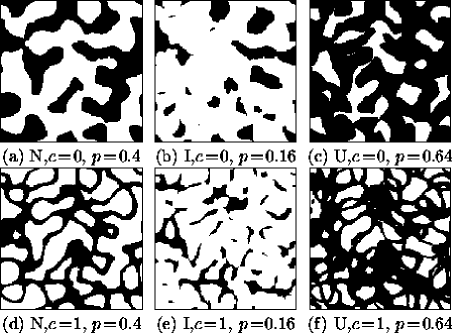
FIG. 1.: Six different microstructures generated by the level-cut scheme. In the top row we show a one-cut field and its intersection and union with a statistically identical structure. In the bottom row we show analogous structures derived from a two-cut field. The images have a side length of 10$\mu$m.

FIG. 2.: The theoretical (lines) and measured (symbols) correlation functions of the six models shown in Fig. 1. The squares correspond to the models constructed from one-cut fields (Figs. 1a-c), and the triangles to the the two-cut fields (Figs. 1d-f).

give nine primary classes of microstructure with which to compare real composites. These broadly cover the types of morphology obtainable by combining two composites generated by the level-cut GRF scheme.

II Statistical reconstruction

The two most common experimentally measured morphological quantities of composites are the volume fraction $p_{exp}$ and the two-point correlation function $p_{exp}^{(2)}(r)$ (eg. Refs. [6, 21, 23, 39, 40]). Consider how this information might be used to reconstruct the composite using the simple one-cut GRF model (model N, $c\!=\!0$ or $\alpha\!=\!-\infty$). The level-cut parameter $\beta$ can be obtained by solving $p_{exp}=(2\pi)^{-\frac{1}{2}}\int_{-\infty}^{\beta}e^{-t^{2}/2}dt$ and the field-field function obtained by numerical inversion of

$$p_{exp}^{(2)}(r)=p_{exp}^{2}+\frac{1}{2\pi}\int_{0}^{g(r)}\frac{dt}{\sqrt{1-t^{2}}}\exp\left({-\frac{\beta^{2}}{1+t}}\right).$$ (15)

From $g(r)$ we can obtain $\rho(k)$ by inverting Eq. (2) and using either Eq. (1) or (3) to obtain $y(\mbox{\boldmath$r$})$ and hence the model phase function $\phi(\mbox{\boldmath$r$})$. The reconstruction shares first and second order statistical properties with the image and would therefore be expected to yield a reasonable model of the original composite. This is similar to the procedure of Quiblier [19] employed in previous studies [5, 6, 10, 20, 21, 22, 23] although the formulation of the model is different. There are several operational problems with this reconstruction procedure. First, the numerical inversion of Eq. (15) may not be robust or well defined. Furthermore experimental error in $p^{(2)}_{exp}(r)$ is carried over to $g(r)$. Second, the inversion of Eq. (15) may yield a spectral density $\rho(k)$ which is not strictly positive. We now generalise the method to incorporate the models N, I and U of § I and show how these problems can be avoided.

First select one of the three models (N, I or U) and a value of $c$=$0$, $\frac{1}{2}$ or $1$ (giving a total of nine combinations) so that $\alpha$ and $\beta$ are fixed by $p_{exp}$. It remains to find $g(r)$. Instead of inverting an analog of Eq. (15) we assume this function is of the general form given by Eq. (11) (this guarantees that $\rho(k)$ is positive). The three length scale parameters are obtained by a best fit procedure which minimises the normalised least-squares error;

$$Ep^{(2)}=\sum_{i=1}^{M}[p^{(2)}_{fit}(r_{i})-p^{(2)}_{exp}(r_{i})]^{2}/\sum_{i=1}^{M}[p^{(2)}_{exp}(r_{i})-p_{exp}^{2}]^{2}.$$ (16)

Here $p^{(2)}_{fit}(r_{i})=p^{(2)}[g(r_{i};r_{c},\xi,d)]$ is the correlation function appropriate for model N, I or U. Once $r_{c}$, $\xi$ and $d$ have been obtained the reconstruction $\phi(\mbox{\boldmath$r$})$ can be generated. If the one-cut model (N, $c\!=\!0$) is chosen we assume that the results will not differ significantly from those obtained using Quiblier’s method.

To illustrate the procedure we reconstruct a material with known statistical properties. For this purpose we choose a normal two-cut GRF model with $p_{\alpha,\beta}=0.4,0.6$ (ie. model N, $c=1$) obtained from the field-field function [7]

$$g(r)=e^{-(r/l_{0})^{2}};\;\;\;\rho(k)=\frac{l_{0}^{3}}{(4\pi)^{\frac{3}{2}}}e^{-(kl_{0}/2)^{2}}$$ (17)

with $l_{0}=2.0\mu$m. The “experimental” data for the reconstruction $p^{(2)}_{exp}(r_{i})$ are evaluated using Eq. (6) at $80$ points distributed uniformly on the interval $[0,4]\mu$m (shown as symbols in Fig. 3). The minimisation algorithm is used to find $r_{c}$, $\xi$ and $d$ for four different models. Numerical results are reported in Table I and the best-fit functions $p^{(2)}_{fit}$ are plotted in Fig. 3. Each of the models is able to provide an excellent fit of the data. As expected, model N ($c=1$) provides the least value of $Ep^{(2)}$. However the

TABLE I.: The parameters obtained in the reconstruction procedure (Eq. (16)) of a test composite. The surface area of the original model is $0.87\mu$m^-1. Here, and in subsequent tables, $n(m)$ denotes $n\!\times\!10^{-m}$.

Cl	$c$	$r_{c}$	$\xi$	$d$	$Ep^{(2)}$	$s_{fit}$
N	0	0.4033	0.4031	7.7069	1(-3)	1.13
N	1	2.3702	2.3688	6.2140	3(-5)	0.89
I	1	0.9739	0.9729	9.1032	4(-4)	1.05
U	1	4171.1	6651.8	8.3899	4(-3)	0.98

FIG. 3.: The correlation functions $p_{fit}^{(2)}(r)$ (lines) of four reconstructed models obtained by fitting “experimental” data (symbols).

relative improvement over the other three models is not large, and probably of little significance in the presence of experimental error. Cross-sections of the original composite and the reconstructions are shown in Fig. 4(a)-(e). The extremely different morphologies exhibited by the reconstructions provide a graphical illustration of the non-uniqueness of $p^{(2)}(r)$. Therefore for prediction of macroscopic properties (which will differ dramatically for materials shown in Fig. 4) it is necessary to find a more discriminating method of distinguishing composites. From the cross-sectional images the best candidates appear to be models N ($c\!=\!1$) and U ($c\!=\!1$) shown in Figs. 4(c) and (e). Obviously it is preferable to establish some quantitative test to choose the best representation.

A second useful illustration of the method is provided by reconstructing a material with a strongly oscillating correlation function. For this case we take as a test-composite a one-cut model with $p=0.2$ and $p_{\alpha,\beta}=0.0,0.2$ (ie. model N, $c=0$) based on the field-field function [7]

$$g(r) = 3r^{-3}(k_{1}^{3}-k_{0}^{3})^{-1}(\sin k_{1}r-\sin k_{0}r)$$ (19)

$$-3r^{-2}(k_{1}^{3}-k_{0}^{3})^{-1}(k_{1}\cos k_{1}r-k_{0}\cos k_{0}r)$$

$$\rho(k) = 3[4\pi(k_{1}^{3}-k_{0}^{3})]^{-1}[H(k-k_{0})-H(k-k_{1})]$$ (20)

with $k_{0}=3.0$ and $k_{1}=4.5$($\mu$m)^-1. The oscillatory behaviour of the correlation function (see Fig. 5) can only

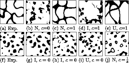
FIG. 4.: Realisations of “experimental” and reconstructed composites. Top row: A material with a monotonicly decaying correlation function (a) compared with four reconstructions (b)-(e). The two point correlation functions of each composite are practically identical (see Fig. 3). Bottom row: A model composite exhibiting an oscillatory correlation function (f) and four reconstructions (g)-(j). In each case the region shown is 10$\times$10$\mu$m.

FIG. 5.: Correlation functions of two reconstructions (lines) of a material exhibiting an oscillatory $p^{(2)}(r)$ (symbols). A “mild” two-cut model (dashed line) is unable to accurately reproduce the strong oscillations.

be reproduced by three of the nine basic microstructures; models N,I and U with $c=0$ (ie. those formed from one-cut fields). For these models $Ep^{(2)}\!<\!0.005$ whereas $Ep^{(2)}\!>\!0.02$ for those based on two-cut structures ($c\!\geq\!\frac{1}{2}$ so $0\!<\!p_{\alpha}\!<\!p_{\beta}$). To illustrate this we show the best fit of a normal two-cut model with $p_{\alpha,\beta}=0.05,0.25$ (N, $c\!=\!\frac{1}{8}$). As can be seen in Fig. 5 this “mild” two-cut model (shown as a dashed line) cannot reproduce the behaviour of the experimental data (see Table II). Realisations of the original material and reconstructions are shown in Fig. 4(f)-(j). Each appears to provide a reasonable representation.

In contrast to the case of a monotonicly decaying $p^{(2)}(r)$ (which was reproduced by four distinct models) strong oscillations appear to be a signature of morphologies generated by the single level-cut model. Unless there exists some reason to employ models U and I in such a case it is likely that the standard one-cut GRF (ie. the model employed in prior studies) will be appropriate.

TABLE II.: Reconstruction of a normal one-cut model with an oscillatory correlation function. Models formed from two-cut fields (ie. $p_{\alpha}>0$) were unable to reproduce the oscillations of $p^{(2)}(r)$ (see eg. row 4). The surface area of the original model is $1.00\mu$m^-1.

Cl	$c$	$r_{c}$	$\xi$	$d$	$Ep^{(2)}$	$s_{fit}$
N	0	1.6326	1.6330	1.6586	2(-4)	1.01
I	0	2.8276	2.8305	1.7220	4(-3)	1.20
U	0	3.9019	3.8935	1.7263	4(-3)	1.10
N	$\frac{1}{8}$	4.6684	4.6893	1.9215	3(-2)	1.28

There is also a physical basis for this argument when spinodal decomposition plays a role in the microstructural formation. In this case Cahn [41] has shown that the evolution of the phase interface is described by the level-set of a sum of random waves similar to (3).

Finally we comment on the morphological origin of the oscillations, and why they cannot be well reproduced by two-cut models. In Fig. 6 we show $p^{(2)}(r)$ and an image of model N, $c=0$ with $r_{c}$=2, $\xi$=4 and $d$=1$\mu$m. The material has strong oscillatory correlations, these representing the “regular” alternating domains which appear in the image. Compare this with data shown for the two-cut model (N, $c\!=\!\frac{1}{2}$) obtained from the same GRF: the alternating structure is still present but the oscillations are practically extinguished. This is due to the sharper decay (or equivalently the doubled specific surface) associated with the thinner two-cut structures [29]. For comparison we also show a structure with no repeat scale (model N, $c=0$ with $r_{c}$=$\frac{1}{6}$, $\xi$=$\frac{1}{2}$ and $d$=100$\mu$m).

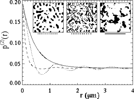
FIG. 6.: Three different types of microstructure. A one-cut model with a well defined domain (or repeat) scale (left), a two-cut model obtained from the same GRF (centre) and a one-cut field with no domain scale (right). The oscillations of $p^{(2)}$ are very weak for the central model even though the domain scale is obvious to the eye.

III Comparison of higher-order statistical properties

We have shown that reconstructions exhibiting quite different morphological properties can share the same two-point correlation function. Here we propose and test three methods with the aim of finding a way of selecting the best reconstruction. Following Yao et al [10] we can compare the three-point correlation function of the model and experimental materials. To do so we define a normalised least-square measure of the error as

$$Ep^{(3)} = \sum_{i=1}^{N_{r}}\sum_{j=1}^{N_{s}}\sum_{k=1}^{N_{\theta}}[p^{(3)}_{fit}(r_{i},s_{j},\theta_{k})-p^{(3)}_{exp}(r_{i},s_{j},\theta_{k})]^{2}$$ (22)

$$\div\sum_{i=1}^{N_{r}}\sum_{j=1}^{N_{s}}\sum_{k=1}^{N_{\theta}}[p^{(3)}_{exp}(r_{i},s_{j},\theta_{k})-p_{exp}^{3}]^{2}.$$

The three-point function $p^{(3)}(r,s,\theta)$ gives the probability that three points distances $r$, $s$ and $t\!=\!(r^{2}+s^{2}-2rs\cos\theta)^{\frac{1}{2}}$ apart all lie in phase one. For our examples we take $N_{r,s,\theta}=8$ with a uniform distribution of $r$ and $s$ on $[0,2]\mu$m and $\theta$ on $[0,\pi]$

A second method of characterising morphology is to calculate microstructure parameters which appear in theoretical bounds on transport and elastic properties [3, 31]. We therefore expect the parameters to contain critical information about the aspects of microstructure relevant to macroscopic properties. These are

$$\zeta = \frac{9}{2pq}\int_{0}^{\infty}\!\!\frac{dr}{r}\int_{0}^{\infty}\!\!\frac{ds}{s}\int_{-1}^{1}\!\!\!du\;P_{2}(u)f(r,s,\theta)$$ (23)

$$\eta = \frac{5\zeta}{21}+\frac{150}{7pq}\int_{0}^{\infty}\!\!\frac{dr}{r}\int_{0}^{\infty}\!\!\frac{ds}{s}\int_{-1}^{1}\!\!\!du\;P_{4}(u)f(r,s,\theta)$$ (24)

where $f(r,s,\theta)=p^{(3)}(r,s,\theta)-p^{(2)}(r)p^{(2)}(s)/p$, $q=1-p$, $u=\cos\theta$ and $P_{n}(u)$ denotes the Legendre polynomial of order $n$. The parameter $\zeta$ occurs in bounds on the conductivity and the bulk modulus, while $\eta$ occurs in bounds on the shear moduli. As $p^{(3)}_{fit}$ and $p^{(3)}_{exp}$ are available for our test models the parameters can be calculated [7, 24]. Techniques have also been suggested for directly evaluating the parameters from experimental images [42, 43]. We anticipate that the closer $\zeta_{fit}$ is to $\zeta_{exp}$ the better the reconstructed model. Note that $\zeta$ and $\eta$ contain only third order statistical information and higher order information is potentially important for our purposes.

A third simple measure of microstructure is the chord-distribution function of each phase [42, 44, 45]. For phase one this is obtained by placing lines through the composite and counting the number of chords $n(r)$ of a given length $r$ which lie in phase one. The chord-distribution is defined as $\rho^{(1)}(r)=n(r)/\int_{0}^{\infty}n(r)dr$ so that $\rho^{(1)}(r)dr$ is the probability that a randomly selected chord will have length between $r$ and $r+dr$. $\rho^{(2)}(r)$ is defined in an analogous manner. At present it is not possible to analytically evaluate this function for the level-cut GRF media, but it can be simply evaluated from realisations of the experimental and reconstructed materials. To quantify the difference between the chord-distributions we again employ a least-squares error;

$$E\rho^{(j)}=\sum_{i=1}^{M}[\rho^{(j)}_{rec}(r_{i})-\rho^{(j)}_{exp}(r_{i})]^{2}/\sum_{i=1}^{M}[\rho^{(j)}_{exp}(r_{i})]^{2}$$ (25)

with $j=1,2$. Note that $\rho^{(j)}(r)$ contains information about the degree of connectedness in phase $j$ and thus is likely to incorporate important information regarding macroscopic properties [46].

We also compute the conductivity of samples (size 128³ pixels) using a finite-difference scheme [7]. We choose the conductivity of phase one as $\sigma_{1}=1$ (arbitrary units) and phase two insulating ($\sigma_{2}=0$). At this contrast the effective conductivity $\sigma$ is very sensitive to microstructure. The results therefore allow us to gauge the ability of a reconstruction to predict macroscopic properties. This contrast also occurs commonly in a range of systems (eg. electrical conductivity of brine saturated porous rocks or thermal conductivity of aerogels and foams).

We have calculated the morphological quantities defined above for the first four reconstructions (reported in Table I). The results are shown in Table III. First note that $Ep^{(3)}$ is greater than $Ep^{(2)}$ by a factor of 2-5 [47] in each case and is probably of little use in an actual reconstruction. The values of the microstructure parameters $\zeta$ and $\eta$ are conclusive; as we expect they indicate that model N ($c=1$) is best. The chord-distributions of the experimental and reconstructed material are shown in Fig. 7 (phase one) and Fig. 8 (phase two). From Table III we see that the chord-distribution provides a very strong signature of microstructure. The results indicate that either model N ($c\!=\!1$) or model U ($c\!=\!1$) is the best reconstruction. The fact that the conductivity of each model is so close to the experimental data provides some evidence that matching the chord distributions is more important than matching $\zeta$ and $\eta$. The same comparison is shown for the reconstructions of the test composite which exhibits an oscillatory $p^{(2)}(r)$ in Table IV. Model N ($c\!=\!0$) provides the best reconstruction based on both the chord-distribution and the microstructure parameters. This leads to a good prediction of the conductivity.

TABLE III.: A comparison of the statistical and transport properties of the four reconstructed models (Table I) with those of the “experimental” composite. The measured surface area of the digital reconstructions is also shown.

Cl	$c$	$Ep^{(3)}$	$\zeta_{fit}$	$\eta_{fit}$	$s_{rec}$	$E\rho^{(1)}$	$E\rho^{(2)}$	$\sigma_{rec}/\sigma_{1}$
N	0	5(-3)	0.32	0.29	1.06	0.25	0.62	0.032
N	1	9(-5)	0.74	0.54	0.75	0.04	0.11	0.114
I	1	2(-3)	0.47	0.37	0.98	0.20	0.48	0.069
U	1	6(-3)	0.87	0.70	1.02	0.02	0.15	0.120
“Exp.” data			0.72	0.54	0.87			0.110

FIG. 7.: The chord-distribution (for phase 1) of an “experimental” composite (Fig. 4a) compared with data for the four reconstructions shown in Figs. 4(b)-(e). Both models N and U ($c=1$) appear to mimic the “experimental” data. The lines in the graph are guides to the eye only.

FIG. 8.: The chord-distribution (for phase 2) of an “experimental” composite compared with data for four reconstructions (see caption of Fig. 7).

In § II we showed that it was possible to generate a number of morphologically distinct reconstructions which share first and second order statistical properties with an experimental composite. Here we have suggested three methods of choosing the best reconstruction. As $Ep^{(3)}$ is relatively small for all seven reconstructions shown in Tables III and  IV, $p^{(3)}$ (like $p^{(2)}$) does not appear to provide a strong signature of microstructure [47]. It is therefore not possible to conclude that a good reproduction of $p^{(3)}$ (or $p^{(4)}$) implies a successful reconstruction as was done in Ref. [10]. In contrast both the chord-distributions and the microstructure parameters appear to provide a strong signature of composite morphology, and hence a method of selecting a useful reconstruction of the original material.

TABLE IV.: A comparison of the statistical and transport properties of the three reconstructed models (Table II) which are able to reproduce the oscillatory correlation function of a test composite.

Cl	$c$	$Ep^{(3)}$	$\zeta_{fit}$	$\eta_{fit}$	$s_{rec}$	$E\rho^{(1)}$	$E\rho^{(2)}$	$\sigma_{rec}/\sigma_{1}$
N	0	9(-5)	0.24	0.20	1.00	0.001	0.003	0.025
I	0	5(-3)	0.33	0.25	1.16	0.137	0.036	0.032
U	0	5(-3)	0.20	0.17	1.10	0.008	0.127	0.009
“Exp.” data			0.24a	0.20a				0.023

IV Reconstruction of the IOS model

Realisations of the identical overlapping sphere (IOS) model [33] (or Poisson grain model [48]) are generated by randomly placing spheres into a solid or void. In the latter case the morphology is thought to provide a reasonable model of the pore-space in granular rocks (so transport occurs in the irregular void region). As the model has a different structure to the level-cut GRF model it provides a useful test of reconstruction procedures [5]. The correlation function of the material [33] is $p^{(2)}(r)=p^{v(r)}$ for $r<2r_{0}$ and $p^{(2)}(r)=p^{2}$ for $r\geq 2r_{0}$ where

$$v(r)=1+\frac{3}{4}\left(\frac{r}{r_{0}}\right)-\frac{1}{16}\left(\frac{r}{r_{0}}\right)^{3}.$$ (26)

For this model it is also possible to calculate the pore chord distribution as $\rho^{(1)}(r)=-3/4r_{0}\times\ln p\;p^{3r/4r_{0}}$ [45].

We first consider the IOS model at volume fraction $p_{exp}=0.2$. The system is 80% filled with spheres of radius $r_{0}$=1$\mu$m. Nine reconstructions are generated (by minimising $Ep^{(2)}$), and their higher order statistical properties are compared with those of the IOS model in Table V. Based on $Ep^{(2)}$ (and $Ep^{(3)}$) we note that models U ($c=\frac{1}{2},1$) perform poorly while the standard one-cut model is very good. The microstructure parameters $\zeta$ and $\eta$ indicate that the best reconstruction is model I ($c=1$) followed by model I ($c=\frac{1}{2}$). However both models fail to reproduce the solid chord distribution ($E\rho^{(2)}>0.6$) which is better mimicked by models I ($c=0$) and N ($c=0$). The ambiguity of the results indicate that none of models considered may be appropriate.

TABLE V.: A comparison of the statistical properties of 11 reconstructions with those of the IOS model at porosity 20%. Most of the models are able to reproduce the low order statistical properties of the IOS model.

Cl	$c$	$Ep^{(2)}$	$Ep^{(3)}$	$s_{fit}$	$\zeta_{fit}$	$\eta_{fit}$	$E\rho^{(1)}$	$E\rho^{(2)}$
N	0	1(-4)	9(-4)	0.94	0.31	0.28	0.066	0.26
N	$\frac{1}{2}$	3(-3)	5(-3)	0.79	0.74	0.54	0.35	0.15
N	1	2(-3)	8(-3)	0.79	0.84	0.63	0.59	0.31
I	0	2(-4)	7(-4)	0.98	0.35	0.30	0.024	0.24
I	$\frac{1}{2}$	6(-4)	1(-3)	1.07	0.50	0.38	0.042	0.65
I	1	4(-4)	1(-3)	1.05	0.52	0.40	0.030	0.63
U	0	2(-4)	1(-3)	0.92	0.28	0.26	0.077	0.30
U	$\frac{1}{2}$	1(-2)	2(-2)	0.91	0.79	0.62	0.49	0.11
U	1	1(-2)	2(-2)	0.91	0.87	0.70	0.40	0.15
I5		7(-4)	6(-4)	1.00	0.40	0.33	0.003	0.23
I10		1(-3)	5(-4)	1.00	0.43	0.35	0.003	0.13
“Exp.” data (IOS)				0.96	0.52	0.42

The IOS model can be thought of as the intersection set of infinitely many composites comprised of a single sphere of phase 2 (so $\phi(\mbox{\boldmath$r$})=0$ within the sphere). This suggests that the morphology may be better modelled with the level-cut scheme by increasing the number of primary composites beyond two. To this end we generalise model I to the case of $n$ independent one-cut fields so that $p^{(2)}(r)=h^{n}(r)$ with $p_{\alpha}=0$, $p_{\beta}=p^{(1/n)}$ and $s=-4np^{1-1/n}h^{\prime}(0)$. This is termed model “I_n”. The statistical properties of the reconstructions for the cases $n$=5 and $n$=10 are shown in rows 10 and 11 of Table V. The models reproduce the “experimental” pore chord distribution very well, and offer a progressively better representation of the solid chord distribution and microstructure parameters. The chord-distributions of model I₅ are shown in Fig. 9 along side those of the standard one-cut model and the IOS model. The good agreement between the measured and theoretical value of $\rho^{(1)}(r)$ for the IOS model demonstrates the accuracy with which this function can be evaluated for a sample of 128³ pixels.

To determine which morphological measure ($\zeta$ and $\eta$ or $Ep^{(1)}$ and $Ep^{(2)}$) should be used to select the best reconstruction we examine the model morphology and conductivity. Three-dimensional images of models N ($c\!=\!0$), I ($c\!=\!1$) and $I_{10}$ are shown alongside the IOS model in Fig. 10. The pore space of the single-cut GRF (Fig. 10a) is more disconnected than that of the IOS model, while the pores are too large and uniform in the intersection model (Fig. 10b). Model I₁₀ (Fig. 10c) appears better able to reproduce the interconnected structures characteristic of overlapping spheres. The results for the conductivity are, $\sigma\!=\!0.038$ for model N ($c\!=\!0$), $\sigma\!=\!0.080$ for model I ($c\!=\!1$), $\sigma\!=\!0.052$ for model I₁₀ and $\sigma\!=\!0.063$ for IOS. The fact that model I₁₀ better mimics IOS morphology and conductivity than model I ($c\!=\!1$) provides evidence that minimising $E\rho^{(j)}$ should be given more weight than matching experimental values of $\zeta$ and $\eta$.

FIG. 9.: The chord distribution of the IOS model (open symbols), model I₁₀ (solid symbols) and the standard one-cut model (broken line, symbols omitted for clarity). The heavy line is the theoretical curve for the IOS model and the lighter lines are guides to the eye only.

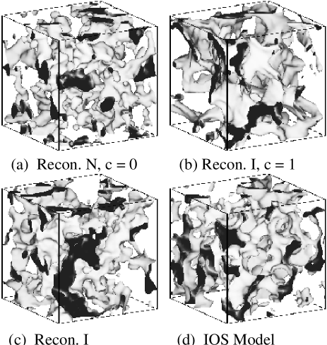
FIG. 10.: Reconstructions of the overlapping sphere (IOS) model at porosity $p=0.2$. To aid visualisation the pores are shown as solid, and solid as void. The images shown here and the chord distributions (Fig. 9) indicate model I₁₀ provides the best reconstruction of the IOS model.

TABLE VI.: The results of the reconstruction procedure for the IOS model. The specific surface of the IOS model is $s=0.71,0.96,1.08,1.10\mu$m^-1 as $p$ increases. Generally model I₁₀ provides a better match of the chord distributions than model I₅. In each case $p_{\beta}\!=\!p^{1/n}$ for model I_n.

$p$	Cl	$r_{c}$	$\xi$	$d$	$Ep^{(2)}$	$s_{fit}$	$E\rho^{(1)}$	$E\rho^{(2)}$
0.1	I5	0.8770	0.8769	3.8336	3(-4)	0.69	0.011	0.33
	I10	1.2472	1.2470	3.8608	5(-3)	0.70	0.011	0.31
0.2	I5	0.9942	0.9947	3.9055	8(-4)	1.00	0.003	0.23
	I10	1.4173	1.4174	3.9777	1(-3)	1.00	0.003	0.13
0.3	I5	1.0974	1.0973	3.9756	1(-3)	1.14	0.003	0.23
	I10	1.6047	1.6053	4.0375	1(-3)	1.13	0.003	0.19
0.4	I5	1.2148	1.2151	4.0250	1(-3)	1.17	0.006	0.16
	I10	1.8146	1.8158	4.1244	1(-3)	1.15	0.004	0.18

We adopt this strategy to reconstruct the IOS model at $p\!=\!0.1$, $0.3$ and $0.4$. In each case models $I_{10}$ and $I_{5}$ provide the best agreement with the experimental chord-distributions. The numerical results are shown in Table VI and cross-sections of each model shown in Fig. 11. We have plotted $p_{fit}^{(2)}(r)$, $p_{exp}^{(2)}(r)$ and measurements of the function from the reconstructed samples in Fig. 12. The measured data shows some deviation from $p_{fit}^{(2)}(r)$ for $p=0.3$. This is due to the accumulation of errors as we form the intersection sets of progressively more phase functions. Conductivity data is given in Table VII and plotted in Fig. 13. Models I₅ and I₁₀ provide a progressively better estimate of the conductivity. We anticipate that increasing the order of model I_n would yield better estimates. The results indicate that we have successfully reconstructed the IOS model.

In Fig. 13 we have also plotted other data for the IOS model. Kim and Torquato [49] (KT) estimated $\sigma$ for the IOS model using a random walker algorithm specifically designed to handle locally spherical boundaries. In the worst case $p=0.1$ our data underestimate that of KT by a factor of 1.6 (the error decreases significantly at higher volume fractions). This is probably due to the discretisation effects of our finite difference scheme [7].

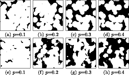
FIG. 11.: The IOS model (a-d) and reconstructions (e-h) which reproduce the correlation function (Fig. 12) and chord-distributions (Fig. 9) of the model. The conducting pore space is shown in black and the images are 10$\times$10$\mu$m.

FIG. 12.: The correlation functions of the IOS model compared with the “best-fit” function associated with each reconstruction. Measurements of $p^{(2)}$ obtained from realisations of the models are also shown.

TABLE VII.: The conductivity of the IOS model and various reconstructions. Models which match the IOS chord-distributions ($I_{5,10}$) provide better estimates of the conductivity than a reconstruction based on the single level-cut model (Rec. N).

$p$	IOS (KT)a	IOS	Rec. N	Rec. I5	Rec. I10
0.1	0.022	0.014	0.003	0.007	0.011
0.2	0.076	0.063	0.038	0.042	0.052
0.3	0.16	0.14	0.094	0.120	0.13
0.4	0.25	0.24	0.180	0.210	0.22

This does not alter our conclusions as all the data presented at a given volume fraction are presumably effected in the same manner. The data of Bentz and Martys [5] (BM) for the IOS model and their one-cut reconstruction are consistently lower than ours.

V Conclusion

We have developed a method of reconstructing three-dimensional two-phase composite materials from information which can be obtained from digitised micrographs. First a range of models are generated which share low order (volume fraction and two-point correlation function) statistical properties with the experimental sample. The model which most closely reproduces the chord-distributions of the experimental material is chosen. The distribution functions provided a better signature of microstructure than the three-point correlation function and are simpler to measure than the microstructure parameters $\zeta$ and $\eta$. Significantly the three-point and higher order correlation functions of the reconstructions can be calculated and employed in rigourous analytical microstructure-property relationships.

FIG. 13.: Conductivity of the IOS model (solid symbols) compared with various reconstructions (open symbols). Model I₁₀ provides a very good prediction of the actual conductivity. Other data are from Refs. [49] (KT) and [5] (BM).

Three-dimensional realisations of the models can also be simply generated for the purpose of numerically evaluating macroscopic properties.

We found that materials with practically identical two point correlation functions can have very different morphologies and macroscopic properties. This demonstrates that reconstructions based on this information alone [5, 6, 10, 18, 19, 20, 21, 22, 23] do not necessarily provide a useful model of the original material. If the correlation function exhibits strong oscillations we found evidence that prior methods will provide satisfactory reconstructions. In this case it is important to compare the chord-distributions of the model and experimental materials.

Our method can be applied to a wider range of composite and porous media than prior reconstruction techniques. The generality of the method is achieved by incorporating new models based on the intersection and union sets of level-cut GRF models. The former have recently been shown to be applicable to organic aerogels [29] and porous sandstones [28], while the latter may be useful for modelling closed-cell foams. Techniques based on the single-cut GRF model cannot reproduce the low percolation thresholds of these materials [24]. The method was successfully used to reconstruct several test composites and the overlapping sphere model over a range of volume fractions. The reconstructions are better able to model the morphology and transport properties of the IOS model than prior studies [5].

There are several problems with the reconstruction procedure. First, it is possible that two materials with different properties may share first and second order statistical information and chord-distribution functions. In this case the reconstruction method could fail to yield good estimates of the macroscopic properties. Second, the generality of the models we have employed is not sufficient to mimic all real composites (although prior studies have shown them to be appropriate for a wide range of materials [24, 25, 26, 27, 28, 29]). An example is provided above where our nine basic reconstructions were unable to model the chord-distribution of the IOS model. In this case a further generalisation was found to be successful. Others are possible. For example, the restriction that the level-cut and length scales parameters are identical for each component of the intersection and union sets can be relaxed, or overlapping spheres can be incorporated in the level-cut scheme. However the problem remains. It is unlikely, for example, that the morphology of randomly packed hard spheres could be mimicked by this scheme. Third, models formed from the union and intersection sets contain sharp edges which are energetically unfavourable in many materials. However there is little evidence that these play a strong role in determining macroscopic properties.

New techniques of characterising microstructure are currently being developed such as those based on information-entropy [48]. These may contribute to the problem of selecting the best reconstructions. Our work also has application to the inverse-problem of small-angle X-ray scattering from amorphous materials. In this case the problem is made more difficult by the absence of higher-order information such as chord-distributions (although some progress may be possible [44]). Work is underway to model anisotropic composites and apply the method to experimental systems.

REFERENCES

- [1]
- [2]
- [3] S. Torquato, Appl. Mech. Rev. 44, 37 (1991).
- [4] M. Sahimi, Rev. Mod. Phys. 65, 1393 (1993).
- [5] D. P. Bentz and N. S. Martys, Trans. Porous Media 17, 221 (1994).
- [6] P. M. Adler, C. G. Jacquin, and J. A. Quiblier, Int. J. Multiphase Flow 16, 691 (1990).
- [7] A. P. Roberts and M. Teubner, Phys. Rev. E 51, 4141 (1995).
- [8] E. J. Garboczi and A. R. Day, J. Mech. Phys. Solids 43, 1349 (1995).
- [9] P. A. Crossley, L. M. Schwartz, and J. R. Banavar, Appl. Phys. Lett. 59, 3553 (1991).
- [10] J. Yao et al., J. Colloid Interface Sci. 156, 478 (1993).
- [11] A. Odgaard, K. Andersen, and F. Melsen, J. Micros. 159, 335 (1990).
- [12] M. J. Kwiecien, I. F. Macdonald, and F. A. L. Dullien, J. Micros. 159, 343 (1990).
- [13] I. F. Macdonald, H. Q. Zhao, and M. J. Kwiecien, J. Colloid Interface Sci. 173, 245 (1995).
- [14] J. T. Fredrich, B. Menendez, and T.-F. Wong, Science 268, 276 (1995).
- [15] P. Spanne et al., Phys. Rev. Lett. 73, 2001 (1994).
- [16] L. M. Schwartz et al., Physica A 207, 28 (1994).
- [17] M. D. Rintoul et al., Phys. Rev. E 54, 2663 (1996).
- [18] M. Joshi, Ph.D. thesis, Univ. of Kansas, Lawrence, 1974.
- [19] J. A. Quiblier, J. Colloid Interface Sci. 98, 84 (1984).
- [20] P. M. Adler, C. G. Jacquin, and J.-F. Thovert, Water Resources Research 28, 1571 (1992).
- [21] M. Ioannidis, M. Kwiecien, and I. Charzis, SPE 30201 (1995), presented at the Society for Petroleum Engineers Petroleum Computer Conference, Houston, 11-14 June.
- [22] M. Giona and A. Adrover, AIChE J. 42, 1407 (1996).
- [23] N. Losic, J.-F. Thovert, and P. M. Adler, J. Colloid Interface Sci. 186, 420 (1997).
- [24] A. P. Roberts and M. A. Knackstedt, Phys. Rev. E 54, 2313 (1996).
- [25] A. P. Roberts and M. A. Knackstedt, J. Mat. Sci. Lett. 14, 1357 (1995).
- [26] M. A. Knackstedt and A. P. Roberts, Macromolecules 29, 1369 (1996).
- [27] A. P. Roberts and M. A. Knackstedt, Physica A 233, 848 (1996).
- [28] A. P. Roberts, D. P. Bentz, and M. A. Knackstedt, SPE 37024 (1996), presented at the Society for Petroleum Engineers Asia Pacific Oil and Gas Conference, Adelaide, 28-31 Oct.
- [29] A. P. Roberts, Phys. Rev. E 55, 1286 (1997).
- [30] W. F. Brown, J. Chem. Phys. 23, 1514 (1955).
- [31] G. W. Milton, Phys. Rev. Lett. 46, 542 (1981).
- [32] P. Debye, H. R. Anderson, and H. Brumberger, J. Appl. Phys. 28, 679 (1957).
- [33] H. L. Weissberg, J. Appl. Phys. 34, 2636 (1963).
- [34] M. Teubner, Europhys. Lett. 14, 403 (1991).
- [35] N. F. Berk, Phys. Rev. A 44, 5069 (1991).
- [36] N. F. Berk, Phys. Rev. Lett. 58, 2718 (1987).
- [37] S. Marčelja, J. Phys. Chem. 94, 7259 (1990).
- [38] M. Teubner and R. Strey, J. Chem. Phys. 87, 3195 (1987).
- [39] J. G. Berryman, J. Appl. Phys. 57, 2374 (1985).
- [40] S. C. Blair, P. A. Berge, and J. G. Berryman, J. Geophys. Res. B 101, 20359 (1996).
- [41] J. W. Cahn, J. Chem. Phys. 42, 93 (1965).
- [42] D. A. Coker and S. Torquato, J. Appl. Phys. 77, 6087 (1995).
- [43] J. Helsing, J. Comp. Phys. 117, 281 (1995).
- [44] P. Levitz and D. Tchoubar, J. Phys. I France 2, 771 (1992).
- [45] S. Torquato and B. Lu, Phys. Rev. E 47, 2950 (1993).
- [46] The fact that contains high-order statistical information (in the sense suggested by the hierarchy of correlation functions) is demonstrated by the following argument. It can be shown that where is the so called lineal-path function [45]. This function expresses the probability that a line of length placed randomly in the material will lie entirely with in phase one. This quantity is approximately equal to the probability that points along a line lie in phase one, ie. it can be obtained from the -point function. As the distance between the points shrinks (ie. ) equality is established.
- [47] In part this can be understood in terms of the close relationship between the functions (e.g. and ). However the fact that and can vary significantly between composites with similar (e.g. Table III) indicates that this function contains distinguishing features of the microstructure: these are just not seen by the measure .
- [48] C. Andraud et al., Physica A 207, 28 (1997).
- [49] I. C. Kim and S. Torquato, J. Appl. Phys. 71, 2727 (1992).