Loops in One Dimensional Random Walks

Abstract

Distribution of loops in a one-dimensional random walk (RW), or, equivalently, neutral segments in a sequence of positive and negative charges is important for understanding the low energy states of randomly charged polymers. We investigate numerically and analytically loops in several types of RWs, including RWs with continuous step-length distribution. We show that for long walks the probability density of the longest loop becomes independent of the details of the walks and definition of the loops. We investigate crossovers and convergence of probability densities to the limiting behavior, and obtain some of the analytical properties of the universal probability density.

I Introduction

One reason for the growing interest in polymers [1] is the desire to understand long chain biological macromolecules, and especially proteins. An important class of polymers is polyampholytes (PAs) [2], which are heteropolymers that carry a mixture of positive and negative charges. In recent years, much attention has been given to the ground state conformations of randomly charged PAs [3, 4]. The study of randomly charged PAs suggests that their ground state has a structure similar to a necklace, made of neutral or weakly charged parts of the chain, compacting into globules, connected by highly charged stretched strings [4]. This structure is a compromise between the tendency to reduce the surface area due to surface tension, and the tendency to expand due to the Coulomb repulsion of the total (excess) charge. A complete analytical characterization of this structure within the necklace model (which was obtained for homogeneously charged polymers [5]), was so far not obtained.

Since a key role in the structure of randomly charged PAs is played by the neutral segments in the chain (forming the beads in the necklace), Monte Carlo (MC) methods were applied to study their size distribution [6, 7, 8, 9]. This problem can be investigated by mapping the charge sequence of the PA into a one-dimensional (1-d) RW. The charge sequence $\omega=\{q_{i}\}\ (i=1,...,N;\ q_{i}=\pm 1)$ is mapped into a sequence of positions $S_{i}(\omega)=\sum_{j=1}^{i}q_{j}$ ($S_{0}=0$) of a random walker (the charges are measured in units of the basic charge, and therefore $q_{j}$ is dimensionless). The random sequence of $N$ charges is thus equivalent to an $N$-step RW, a chain segment with an excess charge $Q$ corresponds to a RW segment with total displacement of $Q$ steps, and a neutral segment is equivalent to a loop inside the RW (see Fig. 1).

Kantor and Ertaş [6, 7, 8] attempted to quantify the necklace model, by postulating that the ground state of a PA will consist of a single globule, formed by the longest neutral segment of the PA, and a tail, formed by the remaining part. However, when the longest neutral segment forms a globule, the typical tail is very large ($\sim N$). Since the tail itself may contain neutral segments, it will further fold into globules, in order to reduce the total energy [9]. This structure is depicted in Fig. 1: The longest neutral segment contains $L$ monomers; it compacts into a globule of linear size proportional to $L^{1/3}$; in the remaining part of the chain the longest neutral segment (the 2nd longest neutral segment) of size $L_{2}$ compacts into a globule of radius $L_{2}^{1/3}$, then the 3rd and so on, until the segments become very small (of only a few monomers). Eventually, all the neutral segments are exhausted and we are left only with strings which carry the PA’s excess charge $Q$, and connect the globules.

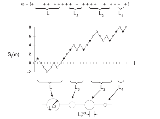
FIG. 1.: An example of a charge sequence $\omega$ (top), mapped into a 1-d RW $S_{i}(\omega)$ (middle), and a typical loops structure (bottom). Filled circles indicate the starting and ending points of loops. The longest loop in the RW has 8 steps ($L=8$), the excess charge (which is equivalent to the total displacement of the RW) is $Q=+8$, and the total length is $N=28$.

There are several models in which a charge sequence is broken into neutral segments (similar to a RW broken into loops) [10]. The relation between these models and the model described above was detailed in a previous work [9], but none of them consider issues of the longest loops.

In this work we investigate the probability density $p(l)$ of a longest loop in an $N$-step RW to be of reduced length $l\equiv L/N$, where $L$ is the number of steps in the loop. This probability density was extensively studied [6, 7, 8, 9], and some of its properties were found analytically. A numerical evidence for the $N$-independence of $p(l)$ in the $N\rightarrow\infty$ limit was presented, but a complete analytical description of it was not found. We present numerical and analytical evidence that this probability density becomes, for long walks, ‘universal’ for a large class of RWs. In order to demonstrate this, we define in section II the problem of the longest loop for RWs with continuous step-length distribution, and in particular we define what is called a loop. We then investigate numerically the crossover from finite $N$ to $N\rightarrow\infty$ for different parameters defining a loop. In section III we demonstrate the ‘universality’ by showing that the probability density of the longest loop becomes, for $N\rightarrow\infty$, independent of $N$, and of the parameter defining a loop, and is the same for both RWs with steps of fixed length and steps of continuous length distribution. In section IV we investigate this ‘universal’ probability density, and obtain some of its properties.

II Longest Loops in Random Walks with Continuous Steps

In this section, unlike the models mentioned in the previous section, we consider the problem of longest loops in RWs with continuous step-length distribution. According to the central limit theorem [11], the end to end distance of a RW, in which the steps are uncorrelated and have finite variance, approaches a Gaussian probability distribution with increasing number of steps. In a long RW we can group a number of adjacent steps into a ‘rescaled step’. If we repeat this rescaling process, the probability distribution of a rescaled step length will approach a Gaussian form. It is, therefore, convenient to start with Gaussian elementary steps, distributed according to probability density $f(x)=e^{-\frac{x^{2}}{2a^{2}}}/a\sqrt{2\pi}$, since the rescaling process does not modify the functional form of the distribution of a step (except for increased variance). We shall denote such a RW, as a Gaussian RW. Although we shall address in this study Gaussian RWs, most of the results will be more general, and valid for large class of RWs with continuous step-length distribution. In Gaussian RWs, the probability density of the position $x$ of the ‘random walker’ after $N$ steps is:

$$f(x,N)=\frac{1}{a\sqrt{2\pi N}}e^{-\frac{x^{2}}{2Na^{2}}}\ ,$$ (1)

where $a^{2}$ is the variance of a single step. Since a RW with continuous distribution of steps never exactly returns to a previously visited position, we say that a loop is closed if two steps in the RW are closer than $\epsilon$ from each other. Therefore, the probability of having a longest loop of $L$ steps in such a RW depends on the number of steps $N$, on the standard deviation of the Gaussian step $a$, and on $\epsilon$ defined above. From dimensional arguments, it is clear that the probability of the longest loop depends on $\epsilon$ and $a$ only through $\epsilon/a$.

As in the problem with fixed step length, it is convenient to work with a probability density of the longest loop, and to explore it as a function of the reduced length $l$. The probability density is defined by $p(l;N,\epsilon/a)=N\cdot P(L;N,\epsilon/a)$, where $P(L;N,\epsilon/a)$ is the probability of having a longest loop of $L$ steps in a RW with given $a$ and $N$, when the distance defining a loop is $\epsilon$.

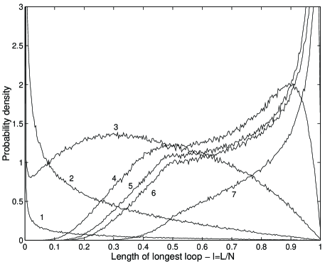
FIG. 2.: $p(l;N,\epsilon/a)$ vs. $l$ for several values of $\epsilon/a$: $10^{-5}$ (1), $10^{-4}$ (2), $10^{-3}$ (3), $10^{-2}$ (4), 0.1 (5), 1 (6), 10 (7). All graphs show MC results of $10^{6}$ randomly selected sequences of length $N=300$.

For a RW with steps of fixed length, it was shown numerically [7] that the probability density of the longest loop becomes $N-$independent already for modest values of $N$. However, the probability density of the longest loop for a RW with continuous step length distribution strongly depends on $\epsilon$. This dependence is depicted in Fig. 2, showing $p(l;N,\epsilon/a)$ for values of $\epsilon/a$ ranging from $10^{-5}$ to 10, and for $N=300$. We now investigate this dependence: The positions of steps of an $N-$step RW are spread out over a distance of order $a\sqrt{N}$. The typical probability of a loop between two given steps for small $\epsilon$ is of order of $\epsilon$ divided by the entire spread of the RW, i.e. $\frac{\epsilon}{a\sqrt{N}}$. Since there are $\sim N^{2}$ pairs of steps which can form a loop, the mean total number of loops in the $\epsilon\rightarrow 0$ limit is of order of $N^{3/2}\epsilon/a$. In the approximation of having no more than one loop per chain ($N^{3/2}\epsilon/a\leq 1$), it is possible to find $p(l;N,\epsilon/a)$ analytically. Neglecting terms ${\cal O}\left[{(\epsilon/a)}^{2}\right]$, the probability density in this single loop (s.l.) approximation is:

$$\begin{array}[]{l}p_{\rm s.l.}(l;N,\epsilon/a)=\\[6.0pt] \sqrt{\frac{2}{\pi}}N^{3/2}\frac{\epsilon}{a}\frac{1-l}{\sqrt{l}}+\left(1-\frac{4}{3}\sqrt{\frac{2}{\pi}}N^{3/2}\frac{\epsilon}{a}\right)\delta(l)\ .\end{array}$$ (2)

We see that when $\epsilon/a\ll 1/N^{3/2}$ no loops are formed, and $p(l;N,\epsilon/a)\simeq\delta(l)$. At the opposite extreme, when $\epsilon/a\gg\sqrt{N}$, every step closes a loop which originates at almost all the other steps in the walk, and therefore the first step generates a loop with the last, resulting in $p(l;N,\epsilon/a)\simeq\delta(l-1)$. And indeed, in Fig. 2 we see that graph 1, representing small $\epsilon/a$, has a strong divergence at $l=0$, while graph 7 shows the signs of strong divergence at $l=1$ (although $\epsilon/a$ is not very big in this case). The intermediate values of $\epsilon/a$ exhibit crossover shapes. In particular we note that graphs 5 and 6, where $\epsilon/a=0.1$ and 1 respectively, have a shape closely resembling the probability density $p(l)$ of the longest loop in RWs with steps of fixed length [7, 9], in the large $N$ limit.

We investigated the $N-$dependence of $p(l;N,\epsilon/a)$, and obtained different qualitative behaviors for different values of $\epsilon/a$. For fixed $\epsilon/a<1$ the function $p(l;N,\epsilon/a)$ changes gradually from $\delta(l)$ towards $p(l)$ as $N$ increases. This behavior resembles that in Fig. 2 (constant $N$ and changing $\epsilon/a$), in a way that increasing $N$ (for constant $\epsilon/a$) is equivalent to increasing $\epsilon/a$ (for constant $N$). For fixed $\epsilon/a>1$, the function $p(l;N,\epsilon/a)$ changes from $\delta(l-1)$ towards $p(l)$ as $N$ increases, in a way that increasing $N$ (for constant $\epsilon/a$) is equivalent to decreasing $\epsilon/a$. At $\epsilon/a\simeq 1$, the probability density $p(l;N,\epsilon/a)$ is almost independent of $N$, and converges very quickly to $p(l)$.

The qualitative arguments of the previous paragraph indicate that for small values of $\epsilon$ the function $p(l;N,\epsilon/a)$ depends on $N$ and $\epsilon/a$ only through $N^{3/2}\epsilon/a$. Numerical comparison of several probability densities, having different values of $N$ and $\epsilon/a$ but the same value of $N^{3/2}\epsilon/a$, confirms this dependence. In the opposite limit $\epsilon/a\gg 1$, we can find through qualitative rescaling arguments a single parameter for the dependence of $p(l;N,\epsilon/a)$ on $N$ and $\epsilon/a$. In order to represent a chain with given $N$, $\epsilon$ and $a$ as a chain with $N^{*}$ ‘effective steps’ and $\epsilon^{*}/a^{*}=1$, we group $n={(\epsilon/a)}^{2}$ steps of the original chain into an ‘effective step’ $a^{*}=a\sqrt{n}=a\sqrt{(\epsilon/a)^{2}}=\epsilon$ (where $\epsilon^{*}=\epsilon$). Since the probability of having a loop of certain length (for loops longer than ${(\epsilon/a)}^{2}$ steps in the original chain) is the same in both chains, then any chain with $N$ steps and $\epsilon/a>1$ can be divided to a chain with $N^{*}=\frac{N}{{(\epsilon/a)}^{2}}$ steps and $\epsilon^{*}/a^{*}=1$ (if $\epsilon/a$ is large enough, so that a rescaling of ${(\epsilon/a)}^{2}$ steps is meaningful, but is nevertheless smaller than $\sqrt{N}$, where $N^{*}$ becomes unity). It is therefore reasonable to assume that for $1\ll\frac{\epsilon}{a}<\sqrt{N}$, the probability density of the longest loop depends only on $N/{(\epsilon/a)^{2}}$. Numerical comparison of several probability densities, having different values of $N$ and $\epsilon/a$ but the same value of $N/{(\epsilon/a)^{2}}$, confirms this dependence.

We want to investigate the dependence of the shapes of the different graphs of $p(l;N,\epsilon/a)$ on $\epsilon/a$ and $N$, and find a fixed point. Since an infinite number of parameters is required to characterize a graph, we simplify the investigation by characterizing each graph by a single parameter $\left<l\right>$ – the average reduced length of the longest loop. Since the functions $p(l;N,\epsilon/a)$, depicted in Fig. 2, are normalized functions which change gradually from $\delta(l)$, where $\left<l\right>=0$ to $\delta(l-1)$, where $\left<l\right>=1$, then $\left<l\right>$ provides a reasonable characterization of the entire probability density for all $l$. Therefore, the fixed point for the entire graph of the function, is obtained when the average $\left<l\right>$ does not change with $N$ and $\epsilon/a$. The dependence of $\left<l\right>$ on $\epsilon/a$ and $N$ is depicted in Fig. 3. The curves in Fig. 3 are lines in the ‘$\epsilon-N$’ plane (on a logarithmic scale), along which $\langle l\rangle$, (calculated by $p(l;N,\epsilon/a)$ from $10^{6}$ random sequences) has constant value.

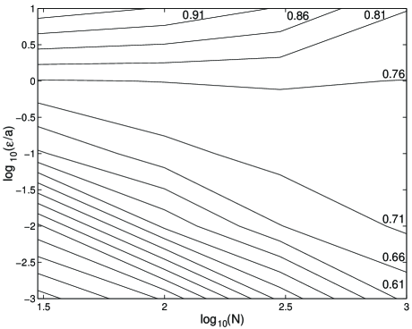
FIG. 3.: Lines along which $\langle l\rangle$ is constant (see text), as a function of $N$ and of $\epsilon/a$ on a logarithmic scale ($N$ = 30 to 1000 and $\epsilon/a$ = 0.001 to 10). The labels above the lines are the average lengths $\langle l\rangle$ along them. The values of $\langle l\rangle$ along adjacent lines differ by 0.05.

It is evident from Fig. 3 that the curves from both sides of the $\epsilon/a\simeq 1$ line are not identical, confirming that the dependence of $p(l;N,\epsilon/a)$ on $\epsilon/a$ is different in value between $\epsilon/a<1$ and $\epsilon/a>1$. The value $\epsilon/a\simeq 1$ is the only value of $\epsilon/a$ for which the probability density is (almost) the same for all $N$ (resulting in $\langle l\rangle\simeq 0.76$). Furthermore, it is evident from the figure that as $N$ increases, $\langle l\rangle$ approaches 0.76 for all values of $\epsilon/a$. It can be shown that as $\langle l\rangle$ approaches 0.76, the probability density $p(l;N,\epsilon/a)$ becomes very similar to $p(l)$. We therefore conclude, that as $N\rightarrow\infty$, the probability density $p(l;N,\epsilon/a)$ becomes independent of the values of $\epsilon$, $a$ and $N$, and very similar to $p(l)$.

In order to demonstrate that the obtained numerical results are not just an effect of a specific definition of what is called a loop, and are typical for RWs with continuous step-length distribution, we repeated the numerical processes for several other definitions of a loop. For instance, we examined the case where the distance defining a loop is a random variable, having different values for every pair of steps. The results obtained for these definitions were very similar to those detailed above. Similar results for several definitions of a loop lead us to the notion that the probability density of the longest loop is ‘universal’, not just in the sense that it does not depend on the values of $\epsilon$ and $a$, but that it does not depend on the details of the definition of what is called a loop.

III Universality of the Probability Density of the Longest Loop

Motivated by the numerical results of the previous section, we try to demonstrate in a more exact way, in what sense the probability density of the longest loop is universal. We first show that for an $N$-step RW with steps of fixed length (discrete RW) this probability density becomes independent of $N$ for large $N$. We then generalize our results to continuous Gaussian RWs.

A Discrete Random Walks

In order to show that the probability density of the longest loop for discrete RWs becomes (for long walks) independent of $N$, we perform a rescaling process: We divide a given long RW with steps of fixed length into $m$ equal sub-walks, which are ‘effective steps’ in the rescaled walk. Each of the $m$ sub-walks has a minimum and a maximum position of steps inside it. A loop between two sub-walks is defined as a loop in the original RW, which starts at a step in one sub-walk, and ends at a step in the second sub-walk. Such a loop is formed when the two sub-walks ‘intersect’ each other (both of them reach the same position). This intersection occurs if either the minimum or maximum of one sub-walk is between the minimum and maximum of the other sub-walk.

The distribution of these minima and maxima depends only on the positions of the first and last steps of each sub-walk, and therefore, the probability of a loop between any two given sub-walks can be calculated analytically for any value of $N$ and $m$. As $N\rightarrow\infty$ the functional forms of the distributions of minima and maxima become simple, and we therefore perform our calculation in that limit. Appendix A describes the calculation of a joint probability density $g(w,W;x)$ of a given RW, ending at a position $x$ relative to its origin, to have a minimum $-w$ and a maximum $W$. This probability density is valid for both discrete RWs and continuous Gaussian RWs, and is depicted in Fig. 4.

However, the calculation of the probability of a loop between two sub-walks does not enable to find the probability density of the longest loop, since it disregards the dependencies between the probabilities of loops. It is therefore convenient to turn to numerical MC methods: We numerically generate independent RWs of $m$ ‘effective steps’, where the distances between their positions are distributed according to a Gaussian probability. Each effective step is assigned random values of a minimum $-w$ and a maximum $W$, according to $g(w,W;x)$, where $x$ is the distance between this step and the next. We can thus obtain all the loops in the RW, and find the longest loop. The probability density of the longest loop is obtained by finding the longest loop for many independent RWs of $m$ ‘effective steps’.

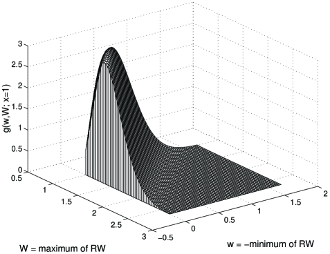
FIG. 4.: Mutual probability density of having a RW with a minimum $-w$ and a maximum $W$: $g(w,W;x=1)$ vs. $w$ and $W$. All lengths are measured in units of the standard deviation of the end position of the RW (see appendix A).

The probability density of the longest loop, emerging from the described rescaling process, converges with increasing $m$ to the $N\rightarrow\infty$ limit of the probability density $p(l)$ of the longest loop for discrete RWs: Apparently, the probability density emerging from the rescaling process should be equal to $p(l)$, since a loop in the rescaled RW is generated if and only if there is a loop in the original discrete RW. However, given a loop between two segments in the rescaled chain, it is impossible to know where in the segments were the ‘original’ steps which generated the loop, and therefore, for each loop in the rescaled chain there is an inherent inaccuracy of up to (plus or minus) one segment. As $m\rightarrow\infty$ this inaccuracy vanishes. This convergence is evident from Fig. 5. We denote the probability density of having a longest loop of length $l=L/m$, in a RW of $m$ ‘effective steps’, by $f_{m}(l)$. We have numerically obtained $f_{m}(l)$ for $m$=4, 10, 20, 50 and 100 (each from $10^{5}$ independent random sequences of length $m$), and compared them to $p(l)$, obtained by MC simulation of $10^{6}$ random sequences of $N=1000$ discrete steps. These functions are depicted in Fig. 5. For each value of $m$, the possible values of $l$ are $\frac{1}{m},\frac{2}{m},\cdots,\frac{m-1}{m}$. The length of the longest loop is never zero, since it can be shown that neighboring sub-walks always make a loop, and is never equal to $m$, since a loop from the first to the last ($m$th) step is $m-1$ segments long. It is evident from Fig. 5 that $f_{m}(l)$ converges very quickly with increasing $m$ to $p(l)$.

The rescaling process described in this section demonstrates the $N-$independence (for large $N$s) of the probability density of the longest loop, for discrete RWs: We can perform this rescaling process to any given discrete (long) RW, and obtain the same probability density of longest loop, independent of the number of steps $N$. Since the rescaling process is statistically exact, the probability density of the longest loop, calculated from the rescaled RW, converges with increasing number of segments to the probability density calculated from the given discrete RW. We therefore conclude that the probability density of the longest loop for discrete RWs becomes independent of $N$ for large $N$.

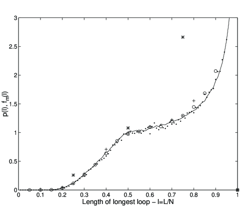
FIG. 5.: $f_{m}(l)$ vs. $l$ for several values of $m$: 4 (star), 10 (plus), 20 (circle), 100 (dot) compared with $p(l)$ (line) as generated by MC simulation of $10^{6}$ random sequences of length $N=1000$.

B Gaussian Random Walks

We now generalize the results, obtained in the previous sub-section for discrete RWs, to continuous Gaussian RWs. Since the calculation of the previous sub-section was conducted in the $N\rightarrow\infty$ limit, the discrete nature of the RW does not affect it. The only difference is that apparently, two segments in a rescaled Gaussian RW can intersect each other, where there is no loop in the original Gaussian RW (this can happen when the positions of steps in one sub-RW which makes a segment are distant more than $\epsilon$, the distance defining a ‘closed loop’, from the positions of steps in the other segment). We demonstrate that such a situation cannot occur: We consider a Gaussian RW of $N$ steps of size $a$, and $\epsilon$ defined above. We scale the positions of steps of the RW by $a\sqrt{N}$, making the distance between the minimum and maximum of order unity. The $N$ steps of the RW are spread along the position axis according to some probability density $q(y)$, where $\int_{\min}^{\max}q(y)dy=1$. The average number of steps of the RW at a certain position $y$ within the (rescaled) interval defining a loop of $\Delta y=\epsilon/(a\sqrt{N})$ is given by:

$$Nq(y)\Delta y=Nq(y)\frac{\epsilon}{a\sqrt{N}}\sim\sqrt{N}\ .$$ (3)

The $\sqrt{N}$ dependence means that the average number of RW steps within the $\Delta y$ interval diverges with increasing $N$, for all the positions along the RW, and for all $\epsilon>0$. We see that in the large $N$ limit the entire range along the position axis is covered by the ‘$\epsilon-$ranges’ (i.e. positions closer than $\epsilon$) of the steps in the Gaussian RW. Therefore, when the minimal or maximal coordinate reached by one Gaussian sub-RW is between the minimum and maximum of another Gaussian sub-RW, it is always closer than $\epsilon$ to a position of a certain step in the second sub-RW, and a loop is formed in the original Gaussian RW.

We can therefore perform the rescaling process of the previous sub-section on a Gaussian RW, and get a probability density of the longest loop, which is identical to the probability density for discrete RWs. We have thus shown that the probability density of the longest loop (for large enough $N$s) is independent of $N$ and is the same for both discrete RWs and Gaussian RWs, when a loop is defined according to an arbitrary $\epsilon>0$. We therefore conclude that this probability density has some measure of ‘universality’.

IV Properties of the ‘Universal’ Probability Density

In the previous section we numerically obtained the probability density of the longest loop through a rescaling process. Although we cannot find this probability density analytically, there are some properties and related probabilities that can be found analytically.

Since a loop between two sub-walks in a discrete RW is formed if the two sub-walks intersect, we want to calculate the probability of such intersection. Fig. 6 depicts two such sub-RWs (solid lines), which are part of one long RW (dashed line).

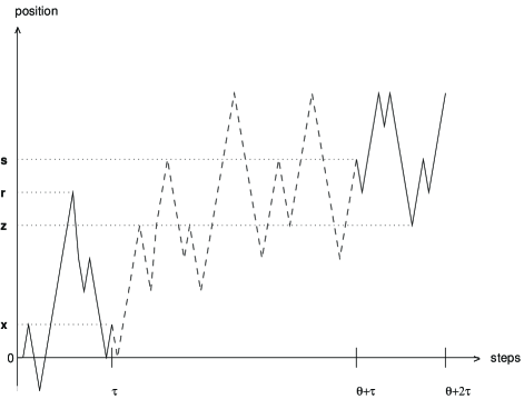
FIG. 6.: Two discrete RWs (solid lines), each of $\tau$ steps, which are sub-walks of a single RW (connecting dashed line). The origin of the second walk is shifted $s$ along the position axis. See text for explanations of other labels.

Each sub-walk is a discrete RW, having $\tau$ steps of size $a$. (We are interested in the limit where $\tau\rightarrow\infty$ and $a\rightarrow 0$ so that $a\sqrt{\tau}$ is finite.) The position of the last step of the first sub-RW is $x$, while the second sub-RW begins at a position $s$ relative to the origin, and $\theta$ steps (along the original RW) after the first sub-RW ends. The two sub-walks intersect (forming a loop in the original RW) if and only if $r$, the maximum of one walk (the first walk in Fig. 6) is greater or equal to $z$, the minimum of the other walk.

These sub-walks are not independent RWs: Fixing the position $s$ of the origin of the second sub-walk affects the probabilities of the possible states of the first sub-walk (and specifically the probability of the end-step position), thus making it not completely random. This ‘dependence’ between the sub-walks is stronger when the number of steps $\theta$ between them is small. In the extreme case, of neighboring sub-walks (i.e. $\theta=0$ and the second sub-walk begins where the first one ends), the end-position of the first sub-walk is fixed to be equal $s$. The probability of a loop between two ‘dependent’ sub-walks, separated by $\kappa$ sub-walks along the original RW (i.e. $\theta=\kappa\tau$ in Fig. 6), denoted by $P_{\rm RW}(\kappa,\Delta\equiv\frac{s}{a\sqrt{\tau}})$, is derived in appendix B and depicted in Fig. 7.

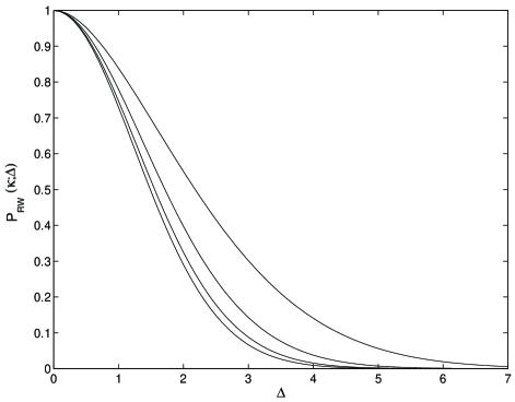
FIG. 7.: Probability of a loop between two sub-walks $P_{\rm RW}(\kappa,\Delta)$ as a function of the normalized distance between their origins $\Delta=\frac{s}{a\sqrt{\tau}}$ and the number of sub-walks between them $\kappa$ (see text). Different lines for different values of $\kappa$ (from top): 1, 3, 10, $\kappa\rightarrow\infty$.

We can now calculate the probability of a loop between any two sub-walks in a RW, and therefore the probability of having a loop of a given length. However, this calculation does not enable us to find the probability density of the longest loop, since it disregards the dependencies between the probabilities of loops: The fact that there is a loop (or that there are no loops) between two other sub-walks in the RW, changes the probability $P_{\rm RW}(\kappa,\Delta)$, of having a loop between two sub-walks, resulting in an expression that we cannot find analytically.

Although we cannot find an analytical expression for $p(l)$, the probability density of the longest loop, we can find some of its analytical properties in the limit of long loops (i.e. $l\rightarrow 1$). We divide a RW with $N$ steps of fixed length $a$ into $m$ segments of $\tau$ steps, and investigate $f_{m}(\frac{m-1}{m})$, the probability of having a loop between the first and the last segments. When the last segment’s origin is shifted $s$ from the origin of the RW, the probability of a loop between the first and last segments is $P_{\rm RW}\left(\kappa=m-2,\ \Delta=\frac{s}{a\sqrt{\tau}}\right)$. In order to obtain the probability of a loop between the first and last segments, $P_{\rm RW}$ is integrated over all possible values of $s$ with the probability of the RW to reach $s$ after $m-1$ segments. The resulting probability is:

$$f_{m}\!\left(\!\frac{m-1}{m}\!\right)\!\!=\!\!\frac{1}{\sqrt{2\pi(m\!-\!1)}}\int_{-\infty}^{\infty}\!\!\!\!\!\!d\Delta e^{-\frac{1}{2}\frac{\Delta^{2}}{m-1}}P_{\rm RW}\left(m\!-\!2,\Delta\right)\!\!\!\ .$$ (4)

In the $m\rightarrow\infty$ limit, Eq. (4) becomes:

$$f_{m}\left(\frac{m-1}{m}\right)\!=\!\frac{1}{\sqrt{2\pi m}}\int_{-\infty}^{\infty}\!\!\!\!\!d\Delta\lim_{m\rightarrow\infty}P_{\rm RW}(m,\Delta)\!\!\simeq\!\!\frac{3.2}{\sqrt{2\pi m}}\ .$$ (5)

Substituting $l_{0}=\frac{m-1}{m}$ in Eq. (5), we get:

$$f_{m}(l_{0})\simeq\frac{3.2}{\sqrt{2\pi}}\sqrt{1-l_{0}}\ .$$ (6)

The behavior of $p(l)$ in the $l\rightarrow 1$ limit was obtained by Kantor and Ertaş [7]:

$$p(l)=\frac{A}{\sqrt{\pi(1-l)}}\ ,$$ (7)

where $A$ is a numerically obtained constant ($A=1.011\pm 0.001$). This means that the probability $P_{l_{0}}$ of a loop to be longer than $l_{0}$ is (in the $l_{0}\rightarrow 1$ limit):

$$P_{l_{0}}=\int_{l=l_{0}}^{1}p(l)dl=\frac{2}{\sqrt{\pi}}A\sqrt{1-l_{0}}\ .$$ (8)

It is evident (by comparing Eqs. (6) and (8) ) that the $l-$dependence of $f_{m}(l)$ is in accordance with the behavior of $p(l)$ in the $l\rightarrow 1$ limit obtained in [7].

Any loop longer than $m-1$ segments in the RW begins at the first segment and ends at the last one, and is therefore ‘counted’ by $f_{m}(\frac{m-1}{m})$. On the other hand, all the loops that are between the first and the last segments of the RW are longer than $\frac{m-2}{m}$ of the chain. We therefore get for all $m$:

$$P_{l_{0}=\frac{m-1}{m}}<f_{m}\left(\frac{m-1}{m}\right)<P_{l_{0}=\frac{m-2}{m}}\ .$$ (9)

In the $m\rightarrow\infty\ ,l_{0}\rightarrow 1$ limit we get by substituting the definitions of $P_{l_{0}}$ and $f_{m}(\frac{m-1}{m})$ to Eq. (9):

$$\frac{2}{\sqrt{\pi}}A\frac{1}{\sqrt{m}}<\frac{3.2}{\sqrt{2\pi m}}<\frac{2}{\sqrt{\pi}}A\sqrt{\frac{2}{m}}\ .$$ (10)

From Eq. (10) we can obtain analytical upper and lower bounds on $A$:

$$0.80<A<1.13\ ,$$ (11)

which are satisfied by the known numeric value of $A=1.011$ obtained in [7].

V Conclusions and Discussion

We have defined the problem of the longest loop for RWs with continuous step-length distribution, investigated the resulting probability densities, and showed that they converge with increasing number of steps in the RW to the probability density of the longest loop in RWs with steps of fixed length. These results motivated a rescaling process, which enabled us to obtain a probability density of the longest loop, which is independent of the number of steps and of the nature of the single step of the RW. We have presented numerical and analytical evidence, suggesting that this probability density is identical for both discrete and continuous RWs. Investigating this ‘universal’ probability density, we have obtained some of its analytical properties in the limit of long loops. It may be possible to establish additional analytical properties of the problem, through further investigation of this universal function. However, a full renormalization–group treatment of the problem within the derived rescaling process, in order to find a complete analytical solution to the problem, is expected to be quite complicated, since we are interested in an entire probability density and not in a single parameter.

We note that the entire rescaling process described in this work is applicable only to 1-d RWs. Since for RWs in dimensions $\geq 2$ there is no analog to the minimum and maximum (there is no ‘boundary’ to the RW), we cannot perform the rescaling process (for both discrete and Gaussian RWs), and the results do not apply to such RWs.

The rescaling process, leading to a ‘universal’ probability density of the longest loop, leads, in a similar way, to a ‘universal’ probability density of the second longest loop (and third longest loop, and so on). The definitions and processes of section III can be used in order to obtain the probability density of the second longest loop: When we performed the rescaling process, we first obtained all the loops in the rescaled RW, and only then the longest loop. Therefore, after ‘erasing’ the longest loop, the second longest loop can be obtained, and then the third, and so on. In Fig. 8 the probability density (from $10^{5}$ random sequences) of the second longest loop of a rescaled chain, having $m=20$ segments, is compared to the same probability density of a discrete RW of $N=1000$ steps, obtained by MC simulation of $10^{6}$ random sequences. As expected, these probabilities are very similar.

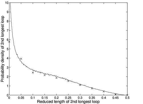
FIG. 8.: Probability density of the second longest loop of a rescaled chain of $m$=20 segments ($\times$), compared with the probability density of the second longest loop of a discrete RW of $N$=1000 steps (line).

The ‘universality’ demonstrated in this study means that the probability densities of longest loops are independent of the number of steps and of the nature of the single step of the RW. Therefore, by mapping the 1-d RW into the charge sequence of a polymer, we see that the results obtained in previous works for a specific case of randomly charged PAs [6, 7, 8, 9] are valid for a larger class of randomly charged polymers.

A Mutual Probability of a Minimum and Maximum of a Random Walk

We present the derivation of the mutual probability of the minimum and maximum of a RW. The probability of the position of a ‘random walker’ satisfies the diffusion equation, and the problem of a ‘random walker’ bound between a minimum and a maximum can be represented as a diffusion between absorbing walls [11, 12]. We solve the diffusion equation in one dimension [13]:

$$\frac{a^{2}}{2}\frac{\partial^{2}f(x,t)}{\partial x^{2}}=\frac{\partial f(x,t)}{\partial t}\ ,$$ (A1)

for the probability density $f(x,t)$ of a particle starting at the origin and taking steps of size $a$ to be at a position $x$ after $t$ steps, with boundary conditions of vanishing $f$ at $-w$ and $W$. The eigenfunctions are of the form:

$$\sin\left(\frac{n\pi(w+x)}{w+W}\right)e^{-\frac{1}{2}\left(\frac{n\pi}{w+W}\right)^{2}a^{2}t}\ ,$$ (A2)

and the prefactors are determined from the initial condition $f(x,t=0)=\delta(x)$. The resulting probability density (with respect to $x$) $f_{w,W}(x,t)$ of a RW to be at a position $x$ after $t$ steps, when there are absorbing walls at $-w$ and $W$, is given by:

$$\begin{array}[]{l}f_{w,W}(x,t)=\\[6.0pt] \frac{2}{w+W}\sum_{n=1}^{\infty}\sin\left(\frac{n\pi w}{w+W}\right)\sin\left(\frac{n\pi(w+x)}{w+W}\right)e^{-\frac{1}{2}\left(\frac{n\pi}{w+W}\right)^{2}a^{2}t}\ .\end{array}$$ (A3)

We are interested in the conditional probability of a given RW to have a maximum lower than $W$, and a minimum higher than $-w$. This conditional probability is equal to the derived probability density $f_{w,W}(x,t)$, divided by the probability density $f(x,t)$ of the RW to be at a position $x$ after $t$ steps. When measuring all distances (i.e. $w$, $W$ and $x$) in units of $a\sqrt{t}$, we get for the conditional probability:

$$\begin{array}[]{l}G(w,W;x)=\\[6.0pt] \frac{2\sqrt{2\pi}}{w+W}e^{\frac{x^{2}}{2}}\sum_{n=1}^{\infty}\sin\left(\frac{n\pi w}{w+W}\right)\sin\left(\frac{n\pi(w+x)}{w+W}\right)e^{-\frac{1}{2}\left(\frac{n\pi}{w+W}\right)^{2}}\ .\end{array}$$ (A4)

The derivative of $G$ in respect to $w$ and $W$:

$$g(w,W;x)=\frac{\partial^{2}G(w,W;x)}{\partial w\partial W}\ ,$$ (A5)

is the mutual probability density (in respect to $w$ and $W$) of a given RW, ending at a position $x$, to have a minimum $-w$ and a maximum $W$. This derivation of $g(w,W;x)$ can be repeated for a continuous Gaussian RW with step size $a$, and therefore the mutual probability density $g(w,W;x)$ is also valid for Gaussian RWs. Fig. 4 in section III depicts this probability density.

B Probability of an ‘Intersection’ Between Random Walks

We present the derivation of the probability of an ‘intersection’ between two RWs, that are sub-walks of one RW with steps of fixed length. Such an intersection indicates that a loop is formed between the two sub-walks (see Fig. 6 in section IV). The probability of a loop is derived for an infinitely long RW, where each sub-walk can be treated within the Gaussian statistics. We use the notations of section IV – the number of steps in each sub-walk is $\tau$, the size of each step is $a$, there are $\kappa\tau$ steps of the RW between the two sub-walks, the end position of the first sub-walk is $x$, and the second sub-walk begins at a position $s$ relative to the origin of the first sub-walk. Without loss of generality we can suppose that $s\geq 0$. The two sub-walks form a loop when the maximal coordinate of the first walk is greater or equal to the minimal coordinate of the second walk (labeled $z$).

The probability density $M(r,\tau)$ of the maximal coordinate of a RW after $\tau$ steps can be shown to be (for $r>0$) twice the probability density of the position of the RW after $\tau$ steps [13]. For $r<0$ the probability density $M(r,\tau)$ vanishes, since the maximum of a RW cannot be lower than its origin. By reflecting each RW about its origin (replacing $+a$ with $-a$ and vise versa), we see that for every RW having a maximum position of $r$, there is a reflected RW having a minimum position of $-r$. Therefore, the probability density $m(r,\tau)$ of the minimal coordinate of a RW after $\tau$ steps equals $M(-r,\tau)$. We thus get:

$$M(r,\tau)=m(-r,\tau)=\left\{\begin{array}[]{ll}2f(r,\tau)=\frac{2e^{-\frac{r^{2}}{2a^{2}\tau}}}{a\sqrt{2\pi\tau}}&,\ {\rm for}\ \mbox{$r\geq 0$}\\ 0&,\ {\rm for}\ \mbox{$r<0$}\end{array}\right.$$ (B1)

where $f(r,\tau)$ is the probability of a RW to be at a position $r$ after $\tau$ steps.

In order to have a loop between the two sub-walks, three independent events must occur:

• The maximal coordinate of the first sub-walk must be greater or equal to the minimal coordinate of the second sub-walk. The probability of a RW to reach a position $x$ and to have a maximum greater than $z$ after $\tau$ steps is given by [11]:

  $$P_{1}(x,z)=\left\{\begin{array}[]{ll}f(2z-x,\tau)&,\ \mbox{for $z\geq\max(0,x)$}\\ f(x,\tau)&,\ \mbox{otherwise}\end{array}\right.\ \ .$$ (B2)

• There is a RW between the end position of the first sub-walk and the origin of the second sub-walk, i.e. a RW of $\kappa\tau$ steps and a total displacement of $s-x$. However, the position $s$ is fixed, and therefore this RW is restricted by the existence of a RW of $\kappa\tau+\tau$ steps from the origin to $s$. This probability is given by

  $$P_{2}(s,x)=\frac{f(s-x,\kappa\tau)}{f(s,(\kappa+1)\tau)}\ .$$ (B3)

• The minimum of the second sub-walk is equal to $z$, i.e $s-z$ relative to its origin. This probability is given by Eq. (B1):

  $$P_{3}(s,z)\!=\!m(z\!-\!s,\tau)\!=\!\!\left\{\begin{array}[]{ll}2f(s\!-\!z,\tau)\!\!\!&\mbox{, for $z\leq s$}\\ 0\!\!\!&\mbox{, for $z>s$}\end{array}\right.\ .$$ (B4)

The probability of a loop, denoted by $P_{\rm RW}(\kappa,\Delta)$ (for given $s,a,\tau$ and $\kappa$, where $\Delta\equiv s/a\sqrt{\tau})$, is obtained by integration of $P_{1}\cdot P_{2}\cdot P_{3}$ over all values of $z$ and $x$:

$$P_{\rm RW}(\kappa,\Delta)=\int_{z=-\infty}^{\infty}\int_{x=-\infty}^{\infty}P_{1}P_{2}P_{3}dzdx\ .$$ (B5)

From the definitions of $P_{1}$ and $P_{3}$ we see that if $z<0$ then $P_{1}=f(x,\tau)$. If $0\leq z\leq s$ then $P_{1}=f(x,\tau)$ when $x>z$, and if $z>s$ then $P_{3}$ vanishes. Therefore we get:

$$P_{\rm RW}(\kappa,\Delta) =\int_{-\infty}^{0}dzP_{3}(s,z)\int_{-\infty}^{\infty}dxf(x,\tau)P_{2}(s,x)$$ (B8)

$$+\int_{0}^{s}dzP_{3}(s,z)\int_{-\infty}^{z}\!\!dxP_{1}(x,z)P_{2}(s,x)$$

$$+\int_{0}^{s}dzP_{3}(s,z)\int_{z}^{\infty}dxf(x,\tau)P_{2}(s,x)\ .\$$

The resulting probability density is depicted in Fig. 7 in section IV.

REFERENCES

- [1] T. E. Creighton, Proteins: Structures and Molecular Properties, 2nd edn. (W. H. Freeman and Company, New York, 1993); P. G. de Gennes, Scaling Concepts in Polymer Physics (Cornell University Press, Ithaca, New York, 1979); A. Y. Grosberg and A. R. Khokhlov, Statistical Physics of Macromolecules (AIP Press, New York, 1994).
- [2] C. Tanford, Physical Chemistry of Macromolecules (John Wiley and Sons, New York, 1961).
- [3] S. F. Edwards, P. R. King and P. Pincus, Ferroelectrics 30, 3 (1980); P. G. Higgs and J. F. Joanny, J. Chem. Phys. 94, 1543 (1991); Y. Kantor and M. Kardar, Europhys. Lett. 14, 421 (1991); Y. Kantor, H. Li and M. Kardar, Phys. Rev. Lett. 69, 61 (1992); Y. Kantor, M. Kardar and H. Li, Phys. Rev. E 49, 1383 (1994); J. Wittmer, A. Johner and J. F. Joanny, Europhys. Lett. 24, 263 (1993); D. Bratko and A. M. Chakraborty, J. Phys. Chem. 100, 1164 (1996); N. Lee and S. Obukhov, Eur. Phys. J. B 1, 371 (1998); T. Soddemann, H. Schiessel and A. Blumen, Phys. Rev. E 57, 2081 (1998).
- [4] Y. Kantor and M. Kardar, Europhys. Lett. 27, 643 (1994); Y. Kantor and M. Kardar, Phys. Rev. E 51, 1299 (1995); Y. Kantor and M. Kardar, Phys. Rev. E 52, 835 (1995).
- [5] A. V. Dobrynin, M. Rubinstein and S. P. Obukhov, Macromolecules 29, 2974 (1996).
- [6] Y. Kantor and D. Ertaş, J. Phys. A27, L907 (1994).
- [7] D. Ertaş and Y. Kantor, Phys. Rev. E 53, 846 (1996).
- [8] D. Ertaş and Y. Kantor, Phys. Rev. E 55, 261 (1997).
- [9] S. Wolfling and Y. Kantor, Phys. Rev. E 57, 5719 (1998).
- [10] B. Derrida, R. B. Griffiths and P. G. Higgs, Europhys. Lett. 18, 361 (1992); B. Derrida and P. G. Higgs, J. Phys. A27, 5485 (1994); B. Derrida and H. Flyvbjerg, J. Phys. A20, 5273 (1987); B. Derrida and H. Flyvbjerg, J. Phys. A19, L1003 (1986); G. F. Lawler, Duke Math. J. 47, 655 (1980); G. F. Lawler, Duke Math. J. 53, 249 (1986); G. F. Lawler, J. Stat. Phys. 50, 91 (1988); A. J. Guttmann and R. J. Bursill, J. Stat. Phys. 59, 1 (1990); R. E. Bradley and S. Windwer, Phys. Rev. E 51, 241 (1995); D. Dhar and A. Dhar, Phys. Rev. E 55, 2093 (1997).
- [11] W. Feller, An Introduction to Probability Theory and Its Applications, 3rd edn. (John Wiley and Sons, New York, 1968), Vol. 1.
- [12] S. Chandrasekhar, Rev. Mod. Phys. 15, 1 (1943).
- [13] S. Karlin, A First Course in Stochastic Processes (Academic Press, New York, 1966).