Hubbard Fermi surface in the doped paramagnetic insulator

Abstract

We study the electronic structure of the doped paramagnetic insulator by finite temperature Quantum Monte-Carlo simulations for the 2D Hubbard model. Throughout we use the moderately high temperature $T=0.33t$, where the spin correlation length has dropped to $<1.5$ lattice spacings, and study the evolution of the band structure with hole doping. The effect of doping can be best described as a rigid shift of the chemical potential into the lower Hubbard band, accompanied by a transfer of spectral weight. For hole dopings $<20$% the Luttinger theorem is violated, and the Fermi surface volume, inferred from the Fermi level crossings of the ‘quasiparticle band’, shows a similar doping dependence as predicted by the Hubbard I and related approximations.

Since the pioneering works of Hubbard[1], the metal-insulator transition in a paramagnetic metal has been the subject of intense study. Despite this, our theoretical understanding of this phenomenon is quite limited. Hubbard’s original solutions to the problem, the so-called Hubbard I-III approximations, have recently faced some criticism. One fact which is frequently held against his approximations or the closely related two-pole approximations[2, 3, 4, 5] is the difficulty to reconcile them with the Luttinger theorem. This can hardly be a surprise in that all of these approaches rely on splitting the electron creation operator into two ‘particles’ which are exact eigenstates of the interaction term $H_{U}$:

$$c_{i,\sigma}^{\dagger} = c_{i,\sigma}^{\dagger}n_{i,\bar{\sigma}}+c_{i,\sigma}^{\dagger}(1-n_{i,\bar{\sigma}})$$ (1)

$$= \hat{d}_{i,\sigma}^{\dagger}+\hat{c}_{i,\sigma}^{\dagger},$$ (2)

with $[H_{U},\hat{d}_{i,\sigma}^{\dagger}\;]=U\hat{d}_{i,\sigma}^{\dagger}$, and $[H_{U},\hat{c}_{i,\sigma}^{\dagger}\;]=0$. The interaction term is therefore treated exactly, approximations are made to the kinetic energy. This is precisely the opposite situation as compared to the perturbation expansion in $U$, which leads to the Luttinger theorem. At half-filling the two ‘particles’ $\hat{d}_{i,\sigma}^{\dagger}$ and $\hat{c}_{i,\sigma}^{\dagger}$, whose energy of formation differs by $U$, then form the two separate Hubbard bands. The effect of doping in both the Hubbard I approximation or the two-pole approximations consists in the chemical potential cutting gradually into the top of the lower Hubbard band, in much the same fashion as in a doped band insulator. On the other hand the spectral weight along the lower Hubbard band deviates from the free-particle value of $1$ per momentum and spin so that the Fermi surface volume (obtained from the requirement that the integrated spectral weight up to the Fermi energy be equal to the total number of electrons) is not in any ‘simple’ relationship to the number of electrons - the Luttinger theorem must be violated.
In this manuscript we wish to address the question as to what really happens if a paramagnetic insulator is doped away from half-filling, by a Quantum Monte Carlo (QMC) study of the 2D Hubbard model. We use the value $U/t=8$ and work throughout at the moderately high temperature $T=0.33t$. This temperature is small compared to both the bandwidth, $U$, and the gap in the single particle spectrum (see Figure 1). The main effect of $T$ is the destruction of antiferromagnetic order, as discussed in our previous paper[6]. We therefore believe that our study realizes to good approximation the situation for which Hubbard’s solutions were originally designed: a paramagnetic system in the limit of large $U$, at a temperature which is small on the relevant energy scales.
Below, we present results for the single particle spectral function and its doping dependence. These data show, that the Hubbard I approximation is in fact considerably better than commonly believed: the effect of doping indeed consists mainly of a progressive shift of the chemical potential $\mu$ into the band structure of the insulator. The Fermi surface volume, if determined in an ‘operational’ way from the single particle spectral function, indeed is not consistent with the Luttinger theorem.
We start with a brief discussion of the band structure at half-filling, see Figure 1, which shows the single particle spectral function. We note that this is quite consistent with previous QMC work[7]. For comparison the two bands predicted by the Hubbard I approximation,

$$E_{\pm}(\mathchoice{{\hbox{\boldmath$\displaystyle k$}}}{{\hbox{\boldmath$\textstyle k$}}}{{\hbox{\boldmath$\scriptstyle k$}}}{{\hbox{\boldmath$\scriptscriptstyle k$}}})=\frac{1}{2}\;[\;(\epsilon_{\mathchoice{{\hbox{\boldmath$\displaystyle k$}}}{{\hbox{\boldmath$\textstyle k$}}}{{\hbox{\boldmath$\scriptstyle k$}}}{{\hbox{\boldmath$\scriptscriptstyle k$}}}}+U)\pm\sqrt{\epsilon_{\mathchoice{{\hbox{\boldmath$\displaystyle k$}}}{{\hbox{\boldmath$\textstyle k$}}}{{\hbox{\boldmath$\scriptstyle k$}}}{{\hbox{\boldmath$\scriptscriptstyle k$}}}}^{2}+U^{2}}\;]$$ (3)

are also shown as the dashed dispersive lines ($\epsilon_{\mathchoice{{\hbox{\boldmath$\displaystyle k$}}}{{\hbox{\boldmath$\textstyle k$}}}{{\hbox{\boldmath$\scriptstyle k$}}}{{\hbox{\boldmath$\scriptscriptstyle k$}}}}$$=$$-2t(\cos(k_{x})+\cos(k_{y})\;)$ is the noninteracting dispersion). These provide at best a rough fit to those parts of the spectral function which have high spectral weight. Inspection of the numerical spectra shows quite a substantial difference between the numerical and the Hubbard-type band structures: the latter always give two bands, whereas in the numerical spectra one can rather unambiguously identify $4$ of them, denoted as as $B$, $A$, $A^{\prime}$ and $B^{\prime}$ (see the Figure). None of these bands shows any indication of antiferromagnetic symmetry; together with the short spin correlation length[6]

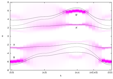
FIG. 1.: Gray-scale plot of the single particle spectral density for the $20\times 20$ cluster at half-filling. The gray scale gives the intensity of spectral weight at the respective $\mathchoice{{\hbox{\boldmath$\displaystyle k$}}}{{\hbox{\boldmath$\textstyle k$}}}{{\hbox{\boldmath$\scriptstyle k$}}}{{\hbox{\boldmath$\scriptscriptstyle k$}}}-\omega$ point. Also shown are the Hubbard I bands (dashed lines) and the $4$-bands obtained by solving (6) (full lines).

this shows that we are really in the paramagnetic phase. We found that to model this $4$-band structure one can inroduce two additional dispersionless bands at energies of $\bar{E}_{\pm}=\frac{U}{2}\pm\epsilon$. We now allow mixing between each of these dispersionless bands and the respective Hubbard band, as would be described by the Hamilton matrix

$$H_{\pm}=\left(\begin{array}[]{c c}E_{\pm}(\mathchoice{{\hbox{\boldmath$\displaystyle k$}}}{{\hbox{\boldmath$\textstyle k$}}}{{\hbox{\boldmath$\scriptstyle k$}}}{{\hbox{\boldmath$\scriptscriptstyle k$}}})&V\\ V&\bar{E_{\pm}}(\mathchoice{{\hbox{\boldmath$\displaystyle k$}}}{{\hbox{\boldmath$\textstyle k$}}}{{\hbox{\boldmath$\scriptstyle k$}}}{{\hbox{\boldmath$\scriptscriptstyle k$}}})\end{array}\right).$$ (6)

Using the values $\epsilon=3t$ and $V=t$, the resulting $4$-band structure provides at least a qualitatively correct fit to the numerical data. We stress that at present we have no ‘theory’ for these two additional bands. Equation (6) is just a phenomenological ansatz to fit the numerical band structure. We note, however, that a $4$-band structure which has some similarity with our results has recently been obtained by Pairault et al. using a strong coupling expansion[8].
We do not, however, pursue this issue further but turn to our main subject, the effect of hole doping. Figure 2 shows the development of $A(\mathchoice{{\hbox{\boldmath$\displaystyle k$}}}{{\hbox{\boldmath$\textstyle k$}}}{{\hbox{\boldmath$\scriptstyle k$}}}{{\hbox{\boldmath$\scriptscriptstyle k$}}},\omega)$ with doping. Thereby the $A(\mathchoice{{\hbox{\boldmath$\displaystyle k$}}}{{\hbox{\boldmath$\textstyle k$}}}{{\hbox{\boldmath$\scriptstyle k$}}}{{\hbox{\boldmath$\scriptscriptstyle k$}}},\omega)$ for different hole concentrations have been overlaid so as to match dominant features, and the chemical potentials for the different hole concentrations are marked by lines. It is quite obvious from this Figure that the $2$ bands seen at half-filling in the photoemission spectrum persist with an essentially unchanged dispersion. The chemical potential gradually cuts deeper and deeper into the $A$ band, forming a hole-like Fermi surface centered on $(\pi,\pi)$, the top of the lower Hubbard band. The only deviation from a rather simple rigid-band behavior is an additional transfer of spectral weight: the part of the $A$-band near $(\pi,\pi)$ gains in spectral weight, whereas the $B$-band looses weight. The loss of the $B$ band cannot make up for the increase of the $A$ band, but rather there is an additional transfer of weight from the upper Hubbard bands, predominantly the $A^{\prime}$ band. This effect is quite well understood[9]. The $A^{\prime}$ band seems to be affected strongest by the hole doping and in fact the rather clear two-band structure visible near $(\pi,\pi)$ at half-filling rapidly gives way to one broad ‘hump’ of weight. Apart from the spectral weight transfer, however, the band structure on the photoemission side is almost unaffected by the hole doping - the dispersion of the $A$-band becomes somewhat wider but does not change appreciably. In that sense we see at least qualitatively the behavior predicted by the Hubbard I approximation.

FIG. 2.: Single particle spectral function for the $8\times 8$ cluster and different electron density $\langle n\rangle$. The chemical potential at half filling is the zero of energy, the spectra for different $\langle n\rangle$ are rigidly shifted relative to one another so as to match dominant features The chemical potentials for the different $\langle n\rangle$ are given by vertical lines.

Next, we focus on the Fermi surface volume. Some care is necessary here: first, we cannot actually be sure that at the high temperature we are using there is still a well-defined Fermi surface. Second, the criterion we will be using is the crossing of the $A$ band through the chemical potential. It has to be kept in mind that this may be quite misleading, because band portions with tiny spectral weight are ignored in this approach (see for example Ref. [10] for a discussion). When thinking of a Fermi surface as the constant energy contour of the chemical potential, we have to keep in mind that portions with low spectral weight may be overlooked. On the other hand the fact that a peak with appreciable weight crosses from photoemission to inverse photoemission at a certain momentum is independent of whether we call this a ‘Fermi surface’ in the usual sense, and should be reproduced by

FIG. 3.: Single particle spectral function for all ${\bf k}$-points of the $8\times 8$ cluster in the irreducible wedge of the Brillouin zone. For each ${\bf k}$ the weight $w_{\bf k}$ is given.

FIG. 4.: Same as Figure 3 for lower electron densities.

any theory which claims to describe the system. It therefore has to be kept in mind that in the following we are basically studying a ‘spectral weight Fermi surface’, i.e. the locus in ${\bf k}$ space where an apparent quasiparticle band with high spectral weight crosses the chemical potential. With these caveats in mind, Figures 3 and 4 show the low-energy peak structure of $A(\mathchoice{{\hbox{\boldmath$\displaystyle k$}}}{{\hbox{\boldmath$\textstyle k$}}}{{\hbox{\boldmath$\scriptstyle k$}}}{{\hbox{\boldmath$\scriptscriptstyle k$}}},\omega)$ for all allowed momenta of the $8\times 8$ cluster in the irreducible wedge of the Brillouin zone, and for different hole concentrations. In all of these spectra there is a pronounced peak, whose position shows a smooth dispersion with momentum. Around $(\pi,\pi)$ the peak is clearly above $\mu$, whereas in the center of the Brillouin zone it is below. The locus in $\textstyle k$-space where the peak crosses $\mu$ forms a closed curve around $(\pi,\pi)$ and it is obvious from the Figure that the ‘hole pocket’ around $(\pi,\pi)$ increases very rapidly with $\delta$. To estimate the Fermi surface volume $V_{F}$ we assign a weight $w_{\bf k}$ of $1$ to momenta ${\bf k}$ where the peak is below $\mu$, $0.5$ if the peak is right at $\mu$ and $0$ if the peak is above $\mu$. Our assignments of these weights are given in Figure 3. The fractional Fermi surface volume then is $V_{F}=\frac{1}{N}\sum_{\bf k}w_{\bf k}$, where $N=64$ is the number of momenta in the $8\times 8$ cluster. Of course, the assignment of the $w_{\bf k}$ involves a certain degree of arbitrariness. It can be seen from Figures 3 and 4,however, that our $w_{\bf k}$

FIG. 5.: Fermi surface volume as estimated from the single particle spectral function, plotted versus the concentration of holes in the half-filled band. The dashed line gives the value predicted by the Luttinger theorem, $V_{F}=\frac{n}{2}$.

would in any way tend to underestimate the Fermi surface volume, so that the obtained $V_{F}$ data points rather have the character of a lower bound to the true $V_{F}$. Even if we take into account some small variations of $V_{F}$ due to different assignments of the weight factors, however, the resulting $V_{F}$ versus $\delta$ curve never can be made consistent with the Luttinger volume, see Figure 5. The deviation from the Luttinger volume is quite pronounced at low doping. $V_{F}$ approaches the Luttinger volume for dopings $\approx 20$%, but due to our somewhat crude way of determining $V_{F}$ we cannot really decide when precisely the Luttinger theorem is obeyed. The Hubbard I approximation approaches the Luttinger volume for hole concentrations of $\approx 50$%, i.e. the steepness of the drop of $V_{F}$ is not reproduced quantitatively. The latter is somewhat improved in the so-called $2$-pole approximation[4, 5]. For example the Fermi surface given by Beenen and Edwards[5] for $\langle n\rangle=0.94$ obviously is very consistent with the spectrum in Figure 3 for $\langle n\rangle=0.95$.
In summary, we have studied the doping evolution of the single particle spectral function for the paramagnetic phase of the 2D Hubbard model, starting out from the insulator. As a surprising result, we found that in this situation the Hubbard I and related approximations give a qualitatively quite correct picture. The main discrepancy between the Hubbard I and the so-called $2$-pole approximation and our numerical spectra is the number of ‘bands’ of high spectral weight, which is $4$ in the numerical data. This is no reason for concern, because we have seen that adding two more bands allows for an quite reasonable fit to the numerical band structure and one might expect that finding a somewhat more intricate decoupling scheme for the Hubbard I approximation or a suitable $4$-pole approximation should not pose a major problem. The greatest success of the Hubbard-type approximations, however, is a qualitatively quite correct description of the evolution of the ‘Fermi surface’. The effect of doping consists of the progressive shift of the chemical potential into the topmost band observed at half-filling, accompanied by some transfer of spectral weight. The Fermi surface volume, determined in an ‘operational way’ from the band crossings, violates the Luttinger theorem for low hole concentrations and does not appear to be in any simple relationship to the electron density. The Luttinger sum rule is recovered only for hole concentrations around $20$%.
It is interesting to note in this context that a recent study of the momentum distribution in the t-J model by high-temperature series expansion[11] has also provided some evidence for a ‘Fermi surface’ which encloses a larger value than predicted by the Luttinger theorem. The criterion used there was a maximum of $|\nabla_{\mathchoice{{\hbox{\boldmath$\displaystyle k$}}}{{\hbox{\boldmath$\textstyle k$}}}{{\hbox{\boldmath$\scriptstyle k$}}}{{\hbox{\boldmath$\scriptscriptstyle k$}}}}n_{\mathchoice{{\hbox{\boldmath$\displaystyle k$}}}{{\hbox{\boldmath$\textstyle k$}}}{{\hbox{\boldmath$\scriptstyle k$}}}{{\hbox{\boldmath$\scriptscriptstyle k$}}}}|$, i.e. the locus of the steepest drop of $n_{\mathchoice{{\hbox{\boldmath$\displaystyle k$}}}{{\hbox{\boldmath$\textstyle k$}}}{{\hbox{\boldmath$\scriptstyle k$}}}{{\hbox{\boldmath$\scriptscriptstyle k$}}}}$. This would in fact be quite consistent with the present results. However, the same caveat as in the present case applies, i.e. this criterion will overlook Fermi level crossings of bands with low spectral weight[10].
In our opinion the strange dependence of $V_{f}$ on electron density makes it questionable whether the ‘spectral weight Fermi surface’ in our data is a true constant energy contour for a system of ‘quasiparticles’. It may be possible that at the temperature we are studying a Fermi surface in the usual sense no longer exists, and that the Hubbard I approximation merely reproduces the spectral weight distribution in this case. As our data show, however, for that purpose the approximation is considerably better than commonly believed.
Zero temperature studies for the doped t-J and Hubbard model are only possible by using exact diagonalization[12], in which case the shell-effects due to the small system size require special care[13, 14]. One crucial point is the very different shape of the quasiparticle dispersion at zero temperature. Whereas the $A$ band is at least topologically equivalent to a nearest neighbor hopping dispersion, with minimum at $(0,0)$ and maxiumum at $(\pi,\pi)$, the zero temperature data[12] show a second-nearest neighbor dispersion with a nearly degenerate band maximum along the antiferromagnetic zone boundary, and a shallow absolute maximum at $(\pi/2,\pi/2)$. The effect of hole doping at zero temperature, however, has a qualitatively very similar effect as in the present case[13]: the chemical potential simply cuts into the quasiparticle band for the insulator, which thus is populated by hole-like quasiparticles[14]. Again, these ‘hole pockets’ violate the Luttinger theorem, indicating again the breakdown of adiabatic continuity in the low doping regime persists also at low temperatures.
We thank W. Hanke for useful comments. This work was supported by DFN Contract No. TK 598-VA/D03, by BMBF (05SB8WWA1), computations were performed at HLRS Stuttgart, LRZ Müchen and HLRZ Jülich.

REFERENCES

- [1] J. Hubbard, Proc. Roy. Soc. A 276, 238 (1963); J. Hubbard, Proc. Roy. Soc. A 277, 237 (1964); J. Hubbard, Proc. Roy. Soc. A 281, 401 (1964).
- [2] L. M. Roth, Phys. Rev. 184, 451 (1969).
- [3] G. Geipel and W. Nolting, Phys. Rev. B 38, 2608 (1988); W. Nolting and W. Borgiel, Phys. Rev. B 39, 6962 (1989).
- [4] B. Mehlig, H. Eskes, R. Hayn, and M. B. J. Meinders, Phys. Rev. B 52, 2463 (1995).
- [5] J. Beenen and D. M. Edwards, Phys. Rev. B 52, 13636 (1995).
- [6] C. Gröber, M. G. Zacher, and R. Eder, cond-mat/9810246.
- [7] R. Preuss, W. Hanke and W. von der Linden, Phys. Rev. Lett. 75, 1344 (1995).
- [8] S. Pairault, D. Senechal, and A.-M. S. Tremblay, Phys. Rev. Lett. 80, 5389 (1998).
- [9] H. Eskes and A. M. Oles, Phys. Rev. Lett. 73 1279 (1994).
- [10] R. Eder and Y. Ohta, Phys. Rev. Lett. 72, 2816 (1994).
- [11] W. O. Putikka, M. U. Luchini, and R. R. P. Singh, Phys. Rev. Lett. 81, 2966 (1998).
- [12] E. Dagotto, Rev. Mod. Phys. 66, 763 (1994).
- [13] R. Eder, Y. Ohta, and T. Shimozato, Phys. Rev. B 50, 3350 (1994); R. Eder and Y. Ohta, Phys. Rev. B 51, 6041 (1994).
- [14] S. Nishimoto, Y. Ohta, and R. Eder, Phs. Rev. B 57, R5590 (1998).