The spectral conductance of a proximity superconductor and the re-entrance effect

Abstract

In a mesoscopic metal in proximity with a superconductor, the electronic conductance is enhanced in a very energy-sensitive way. In this paper, we discuss the spectral conductance of a proximity superconductor from both the theoretical and experimental point of view. The dependence of the spectral conductance on the phase-breaking length, gap of the superconductor and interface transparency is theoretically investigated. We present experimental data on the re-entrance of the normal-state conductance at very low temperature and bias voltage. A complete description of the experimental data needs taking into account heating of the reservoirs by the bias current. In addition, we show that the energy sensitivity of the proximity effect enables one to access the energy distribution of the conduction electrons inside a mesoscopic sample.

1 INTRODUCTION

1.1 The general context

In the past few years, the study of the proximity effect in hybrid structures made of a normal metal in contact with a superconductor has known a remarkable revival.[1, 2, 3] This originated from both the availability of a new generation of tailored-made submicron-sized samples and the new understanding of the coherence effects in electron transport at the mesoscopic scale. The proximity effect is the generic name for the phenomena appearing at the interface of a normal metal (N) with a superconductor (S). In a N-S geometry, the N-metal shows superconducting-like properties including a magnetic screening,[4] a modification of the density of states[5] and an energy-dependent conductance enhancement.[6, 7, 8] In a S-N-S geometry, the Josephson effect is the manifestation of the coherence in the proximity effect. Eventually, the conductance of a N-I-S tunnel junction is governed by the tunneling of electron pairs.

In a N-I-S tunnel junction, the BTK theory[9] describes the cross-over in the behaviour of the interface conductance as a function of tunnel barrier transparency. The interface conductance is twice the normal-state one in the high-transparency limit ($G_{NS}=2G_{NN}$) while it vanishes ($G_{NS}\rightarrow 0$) in the low-transparency limit. The discovery of the zero-bias anomaly[10] showed a clear discrepancy with the BTK theory : in a confined geometry the conductance of the N-I-S junction does not go to zero at zero temperature but increases at low temperature and bias. The physical picture for this effect is that the confinement of electrons by the disorder in the vicinity of the N-S interface makes the transmission probabilities add coherently. This enhances drastically the tunneling of pairs.[11, 12]

Diffusive electron transport in the N metal part of a N-S junction is also significantly enhanced by the proximity effect.[6, 7, 8] The observed large amplitude of the conductance enhancement used to appear in contradiction with the prediction of the Bogoliubov-de Gennes equations[13] and the random matrix theory.[14] The observation of the re-entrance effect has been the key experiment that made the connection between the high-temperature regime and the low-temperature regime.[15, 16, 17, 18] At finite temperature or bias voltage, the conductance of the ”proximity superconductor” made of the N metal in proximity with S is significantly enhanced, while it should coincide with the normal-state value at zero temperature and bias. These features arise clearly from the quasiclassical theory.

In this paper, we will focus on the conductance enhancement in very small N-S structures. We will consider the regime where the N-S interface conductance is large compared to the metallic conductance of the N metal wire. The small size of the structures enables us to investigate the transport properties at temperatures well below the characteristic energy of the proximity effect.

In the following, we will first introduce the main theoretical concepts of the proximity effect. We will concentrate on the spectral conductance and its dependence on various physical parameters. Afterwards, we will present a thorough experimental study of the re-entrance effect in a mesoscopic structure made of a normal metal wire in contact with a superconductor. We will compare our experimental results with the prediction of the theory and conclude about the energy distribution in the reservoirs. Eventually, we will show that the large energy-sensitivity of the proximity effect can be used to test the electron energy distribution inside a mesoscopic sample.

1.2 The Andreev reflection

Let us consider the interface between a normal metal and a superconductor. Well below the superconducting transition temperature of S and at low bias voltage, the thermal energy $k_{B}T$ and the electrostatic energy $eV$ are much smaller than the gap $\Delta$ of S. In this regime, single electrons cannot enter the superconductor because of the absence of avalaible states at the same energy. As a consequence, electrons arriving from N will be Andreev-reflected at the N-S interface, see Fig.1. In this process, the electron is retro-reflected as a hole, while a Cooper pair is transmitted in the superconductor.[19]

At the Fermi energy, the reflected hole has the opposite spin, the opposite velocity and the same momentum as the incident electron. The reflected hole traces back the trajectory of the incident electron. The reflection of a hole may also be seen as the absorption of a second electron. As the Andreev reflection correlates the two electron states, it is equivalent to the diffusion of pairs in the N metal. We call the diffusing pairs in N ”Andreev pairs” as their existence is not due to an intrinsic attractive interaction in N, but to a remote effect which is the Andreev process at the N-S interface.

If one looks more precisely, the reversal of every electron velocity component is perfect only at the Fermi level.[9] Let us consider an electron with a small extra energy $\epsilon$ compared to the Fermi level energy $E_{F}$. The electron wave-vector $k_{e}=k_{F}+q$ is larger than the Fermi wave-vector $k_{F}$. The reflected hole has a slightly different wave-vector $k_{h}=k_{F}-q$, see Fig. 1. This means that the incident and reflected particles will have a difference

$$\delta k=2q=k_{F}\frac{\epsilon}{E_{F}}.$$ (1)

in wave-vector. This difference concerns the wave-vector component which is perpendicular to the N-S interface. With an arbitrary angle of incidence, the change in wave-vector will change the trajectory angle with respect of the N-S interface.[20] In brief, the retro-reflection is imperfect at finite energy.

1.3 The diffusion of ”Andreev pairs”

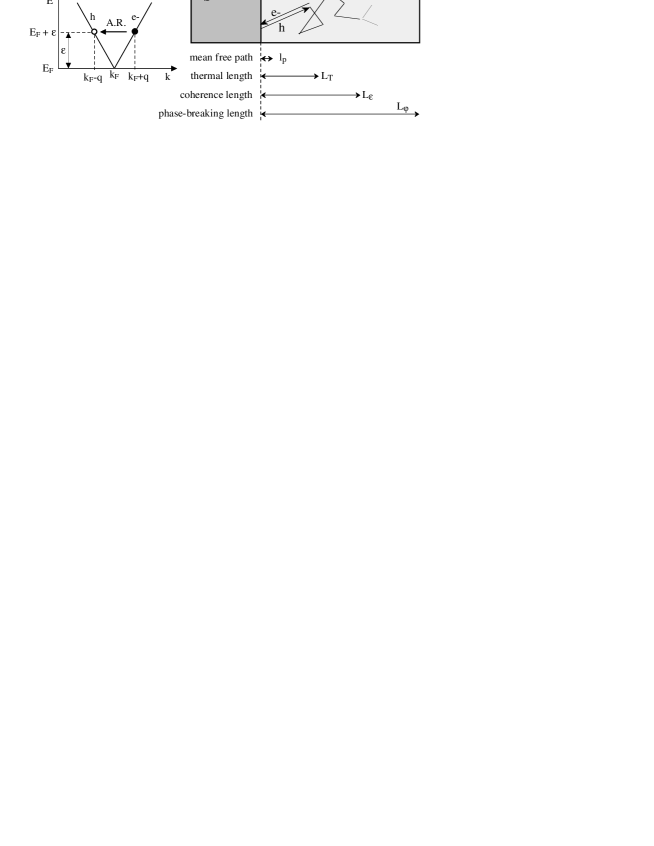
Figure 1: Left : Schematic of the Andreev reflection process. An incident electron with an extra energy $\epsilon$ compared to the Fermi energy $E_{F}$ hits the N-S interface from the N side. The reflected hole-like particle and the incident electron have a slight wave-vector mismatch $2q$. Right : Relevant length scales with their schematic respective amplitudes in a metallic thin film. The energy-dependent coherence length $L_{\epsilon}$ is the length over which the two components of the Andreev pair acquires a phase difference of order $\pi$.

In the following, we will focus on the case of a mesoscopic normal metal in the dirty limit. This means that the elastic mean free path $l_{e}$ is much smaller than the sample length $L$ which is itself smaller than the phase-breaking length $L_{\varphi}$ : $l_{e}\ll L\ll L_{\varphi}$.

Let us consider the trajectories of an electron incoming on the N-S interface and of the reflected hole nearly retracing the trajectory of the incident electron. At zeroth order, the phase acquired by the electron is eaten up as the hole retraces back the trajectory of the incident electron. Looking a little closer, the wave-vector mismatch between the electron and the hole makes the phase difference between the hole and the electron increase monotonically. After diffusion over a distance $L$ from the interface, the phase shift between the two particles is of order $\pi$ at a distance equal to the energy-dependent coherence length :

$$L_{\epsilon}=\sqrt{\frac{\hbar D}{\epsilon}},$$ (2)

$D$ being the diffusion coefficient in N. At the same time, the trajectories of the electron and the hole are shifted by a distance of order the Fermi wavelength.[20] The exact value of the spatial shift depends on the incidence angle on the N-S interface. Further diffusion of the two particles will therefore be different and the pair will break apart. In this respect, the length $L_{\epsilon}$ actually plays the role of the coherence length of the Andreev pair.

The coherence length $L_{\epsilon}$ coincides with the thermal length[21] $L_{T}$ at the energy $\epsilon=2\pi k_{B}T$. The thermal length $L_{T}$ is relevant as soon as one considers the whole electron distribution at thermal equilibrium. This is for instance the case in the Josephson effect. At the Fermi level, the length $L_{\epsilon}$ diverges. Indeed, the coherence length of an Andreev pair is limited by the phase-breaking length $L_{\varphi}$ of a single electron. The average coherence length of an Andreev pair therefore varies from about the thermal coherence length $L_{T}$ at high energy ($\epsilon\simeq k_{B}T$) to the phase-coherence length $L_{\varphi}$ at low energy ($\epsilon\simeq 0$).

The correlation between the electron and the reflected hole can also be described in terms of energy with the equivalence :

$$L_{\epsilon}=L\Leftrightarrow\epsilon=\epsilon_{c}$$ (3)

where

$$\epsilon_{c}=\frac{\hbar D}{L^{2}}$$ (4)

is the Thouless energy, or correlation energy, of a sample of length $L$. The Thouless energy is the fundamental energy scale for the proximity effect at the spatial scale $L$.[7] At a given distance $L$, only electrons with an energy below the Thouless energy are still correlated as Andreev pairs. The other Andreev pairs are broken.

2 THE THEORETICAL BACKGROUND

2.1 The Usadel equation

The diffusion of superconductivity in an inhomogenous structure can be described by the Gorkov Green’s functions. In the limit where all the experimentally relevant length scales are much larger than the Fermi wavelength, the simplification of this fully quantum theory into the quasiclassical theory is valid.[22, 23, 24, 25, 26, 27, 28] The Usadel equations are obtained in the diffusive regime where the elastic mean free path is small. In this framework, weak localization effects and conductance fluctuations are neglected.

Let us restrict to the case of a one-dimensional N-S structure in zero magnetic field and no superconducting phase gradient. The latter condition is fulfilled as soon as there is only one superconducting island. In the absence of electron-electron interaction in N, the Usadel equation in the N metal is :

$$\hbar D\,\delta_{x}^{2}\theta+\{\,2i\epsilon-\frac{\hbar D}{L_{\varphi}^{2}}\,\cos\theta\}\sin\theta=0$$ (5)

The complex proximity angle $\theta=\theta_{1}+i\theta_{2}$ is related to the anomalous Green function $F$ :

$$F(\epsilon,x)=-i\sin[\theta(\epsilon,x)]$$ (6)

The anomalous Green function $F$ is often called the pair amplitude although if differs from the actual pair density which takes into account the energy distribution of the electrons.

The complex angle $\theta$ and the pair amplitude $F$ are functions of both the energy above the Fermi level $\epsilon$ and the distance from the S interface $x$. The Usadel equation features a non-linear diffusion equation for the proximity angle $\theta$. Let us note that the phase-breaking length $L_{\varphi}$ enters the Usadel equations as a cut-off for the proximity effect. The inelastic mean free path $L_{in}$ is included in $L_{\varphi}$, but does not show up by itself. It enters directly in the problem only through the energy redistribution of the electrons in N.

At the contact with an N metal reservoir, the angle $\theta$ is zero. At the contact with a superconducting island S, a complete treatment implies solving the self-consistency equation for the pair potential in the vicinity of the interface.[29, 30] Here we will restrict to the idealized case of a step-like pair potential. The pair potential will be considered as being constant and equal to the gap in S, and zero in N. With this assumption, the boundary condition for a perfectly transparent N-S interface is $\theta=i\pi/2$ at energy zero or well below the gap $\Delta$.

2.2 The spectral conductance

Electron transport is non-local at the mesoscopic scale. In the framework of the quasiclassical theory, the electron transport is nevertheless determined by a local conductivity $\sigma(\epsilon,x)$ which expresses as :

$$\sigma(\epsilon,x)=\sigma_{N}\,\cosh^{2}\theta_{2}(\epsilon,x)$$ (7)

where $\sigma_{N}$ is the normal-state conductivity. From this relation, the local conductivity is always larger than the normal-state conductivity. Since the function $\theta_{2}$ is strongly energy-dependent, so is the conductivity enhancement.

To proceed with transport properties, one needs to know the occupation of current-carrying states. The non-equilibrium quasiparticle energy distribution function can be derived from the out-of-equilibrium Keldysh Green function.[22] The generalized quasiparticle distribution function has two components : an odd part and an even part. The odd part is related to the energy distribution functions of the electrons $f_{e}$ and the holes $f_{h}$ as : $f_{{\it 0}}(\epsilon)=1/2(f_{e}+f_{h})$, and reduces to $\tanh(\epsilon/2k_{B}T)$ at equilibrium. The even part $f=1/2(f_{e}-f_{h})$ is related to the imbalance in the population of holes and electrons, and reduces to zero at equilibrium (no current). It can therefore be named the out-of-equilibrium part of the distribution function.

At any point in a wire of section $S$, the spectral current $i(\epsilon,x)$ is related to the spatial derivative of the distribution function $f$. In this work, we will consider the regime where the inelastic mean free path $L_{in}$ is much larger than the sample length : $L_{in}\gg L$. In this regime, a conduction electron keeps its energy while travelling through the sample. Therefore, the transport channels at different energies are independent and the spectral current $i(\epsilon)$ is constant along the wire. This permits to write the spectral current as a function of the spectral conductance $g(\epsilon)$ and the difference $\Delta f(\epsilon)$ of the distribution functions $f$ at the two extremities of the considered wire :

$$i(\epsilon)=\sigma(\epsilon,x)S\,\frac{df(\epsilon,x)}{dx}=g(\epsilon)\Delta f(\epsilon)$$ (8)

As a consequence, the spectral currents are given by linear circuit theory rules where local voltages are replaced by the electron distribution functions $f$ at the nodes.[23] The spectral conductance $g(\epsilon)$ is the average conductance for electrons with a given energy $\epsilon$ :

$$g(\epsilon)=S[\,\int^{L}_{0}{\frac{dx}{\sigma}}\,]^{-1}=\sigma_{N}S[\,\int^{L}_{0}{\frac{dx}{\cosh^{2}\theta_{2}(\epsilon,x)}}\,]^{-1}=G_{N}+\delta g(\epsilon)$$ (9)

Here, we do not consider the change in conductance of the opened channels with increasing voltage. This was included in the framework of the scattering matrix theory by Lesovik et al.[31]

Let us consider the generic example of a sample made of a quasi-1D N wire ”n” of length $L$ between a S island and a N reservoir, see Fig. 2 inset. The spectral conductance is a measurable quantity, since it coincides with the zero-temperature differential conductance at voltage $V=\epsilon/e$ :

$$g(\epsilon)=\frac{dI}{dV}(V=\epsilon/e,T=0)$$ (10)

The spectral conductance $g(\epsilon)$ is strongly energy-dependent and always larger than the normal-state conductance. In the same way, the excess conductance $\delta g(\epsilon)$ is always positive. At finite temperature, the differential conductance is the integral of the spectral conductance multiplied by the energy derivative of the Fermi distribution function :

$$\frac{dI}{dV}(V=\epsilon/e,T)=\int^{-\infty}_{+\infty}{\frac{d\Delta f}{dV}g(\epsilon)d\epsilon}$$ (11)

This is equivalent to averaging the spectral conductance over an energy window of width $4k_{B}T$.

Real transport experiments involve more complex circuits than the generic two-probe configuration considered above. Let us consider the general case of a network of 1D wires connected to several normal reservoirs and a unique superconducting electrode. The chemical potential of the superconducting island is taken as the reference potential ($V=0$). One can then define a spectral conductance matrix ${\underline{\underline{g}}}$ for the whole circuit connecting the spectral currents matrix ${\underline{i}}$ incoming from the reservoirs with the non-equilibrium distribution functions ${\underline{f}}$ :[32]

$${\underline{i}}={\underline{\underline{g}}}.{\underline{f}}$$ (12)

Integration of this set of relation over the energy gives a direct access to the current-voltage characteristic, since the summation of the spectral currents leads to the measurable current while integration of the $f$ functions of the reservoirs leads to the chemical potential of the reservoirs. Let us note that a zero total current does not mean that the spectral current should be zero. In a reservoir with no injected current, the low-energy and high-energy spectral currents are in general different from zero but cancel out once integrated over the whole energy spectrum.

2.3 The re-entrance effect

As an example for the calculation of the spectral conductance, let us come back to the generic sample geometry made of an N wire between an S island and an N reservoir. The numerical solution of the Usadel equations for the spectral conductance $g(\epsilon)$ in units of the normal-state conductance $G_{N}$ is shown in Fig. 2. From the calculation, the spectral conductance shows a maximum of about $1.15\,G_{N}$ at an energy close to $5.1\,\epsilon_{c}$ with $\epsilon_{c}=\hbar D/L^{2}$. At higher energy, the spectral conductance decays as $1/\sqrt{\epsilon}$. The most striking result is that at zero energy, the normal-state conductance is recovered. This is the re-entrance effect.

The occurance of the re-entrance of the metallic conductance does not depend on the precise sample geometry. It is an exact result from the quasiclassical theory,[23, 24, 25, 26, 27, 28] the random-matrix theory[14, 31] and the Bogoliubov-de-Gennes equations.[28] The zero-energy conductance of a proximity superconductor coincides with the normal-state conductance only in the absence of electron-electron interactions. In the presence of interactions in the normal metal, the zero-temperature conductance is predicted to differ from the normal-state value $G_{N}$. The zero-temperature conductance should decrease in the case of repulsive interactions and increase in the case of attractive ones.[25] The ferromagnetic metals provide a case where the interactions are expected to play a great role in the behaviour of the proximity effect.[33]

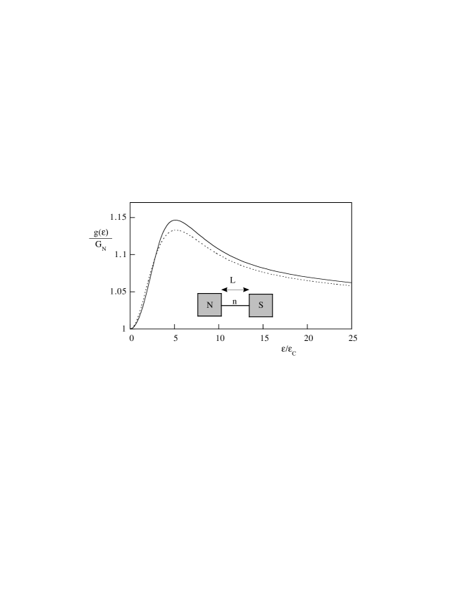
Figure 2: Energy dependence of the spectral conductance $g(\epsilon)$ in units of the normal-state conductance $G_{N}$ for a N-S sample. The sample is made of a normal metal wire ”n” of length $L$ between a N reservoir and a S island, see inset. The spectral conductance was calculated with the help of the full non-linear Usadel equations (full line) and in the linear approximation (dashed line). The gap and the phase-breaking length were assumed to be infinite. The N-S interface transparency is considered as equal to 1.

Let us try to draw a physical picture for the re-entrance effect. The conductivity peak for electrons with a given energy $\epsilon$ appears in the vicinity of the distance $L_{\epsilon}$ from the S interface. Strikingly, it is the point where the Andreev pairs break. At smaller distances $x<L_{\epsilon}$, the Andreev pair is a closed object, i.e. the electron and the hole follow exactly the same path. Another conduction electron cannot enter the Andreev pair. The local conductivity is unchanged by the proximity of the superconductor. The density of states is nevertheless depleted since the probability to find an isolated electron is very small. At a distance $x\simeq L_{\epsilon}$, the electron and the hole have distinguishable trajectories. The Andreev state can couple the electron with a hole a Fermi wave-length away. The hole can even interact again with the superconducting condensate and be reemitted as an electron. This ‘’delocalization” of the electron enhances the local conductivity. At high energy, the conductance enhancement decays because the electron and the hole are increasingly decorrelated.

2.4 The linearization

For the easiness of presentation and understanding, it may be convenient to linearize the Usadel equation and consider the regime of an infinite phase-breaking length. This gives :

$$\hbar D\,\delta_{x}^{2}\theta+2i\epsilon\,\theta=0$$ (13)

The linearization is fully justified only in the case of a (thin) tunnel barrier between N and S. In all cases, it remains a good approximation at a distance from the interface larger than $L_{\epsilon}$.

The linearized Usadel equation is a diffusion equation for the pair amplitude in the real space dimension $x$. The characteristic diffusion length is the coherence length $L_{\epsilon}=\sqrt{\hbar D/\epsilon}$. At a given position x, the characteristic energy scale is $\epsilon_{x}=\hbar D/x^{2}$ which coincides with the Thouless energy $\epsilon_{c}=\hbar D/L^{2}$ in the case $x=L$.

Let us now consider some ideal geometries.

In the case of an semi-infinite length N wire in contact with a S island, the angle $\theta$ has the following simple form :

$$\theta=\frac{\pi}{2}\exp[(i-1)\frac{x}{L_{\epsilon}}]$$ (14)

The local conductivity can be analytically written as :

$$\sigma(\epsilon,x)=\sigma_{N}\cosh^{2}[\frac{\pi}{2}\exp(-\frac{x}{L_{\epsilon}})\sin\frac{x}{L_{\epsilon}}]$$ (15)

In the case of a N wire of finite length, the N reservoir imposes a zero value of $\theta$ at the boundary. Fig. 2 shows the energy dependence of the spectral conductance $g(\epsilon)$ in units of the normal-state conductance $G_{N}$. The curves are calculated without and with the linearization approximation. We observe that the spectral conductance is qualitatively the same in the two cases. Although the linearization does not describe accurately the contribution of low energies, the integrated conductance is very well described. The position and the value of the maxima of conductance are very close in the two calculations. This comparison is the justification for the linear approximation used in Ref. [15].

2.5 Influence of the physical parameters

Let us consider the effect of several physical parameters on the spectral conductance of a sample made of a ”n” metallic wire between one N reservoir and one S island, see Fig. 2 inset.

2.5.1 The phase-breaking length

Figure 3: Energy dependence of the spectral conductance $g(\epsilon)$ in units of the normal-sate conductance $G_{N}$ for various values of the phase-breaking length. Each curve is labeled with the related ratio of the phase-breaking length $L_{\varphi}$ over the sample length $L$. The gap of S is taken as infinite. The barrier transparency is assumed to be $1$.

Up to now, we considered that the phase-breaking length $L_{\varphi}$ is much larger than the sample length $L$. In this case, phase-breaking events have no effect on the spectral conductance since it is the N reservoir which limits the diffusion of pairs in the normal metal wire. Now let us consider the opposite case where the phase-breaking length is smaller than the sample length.

Fig. 3 shows the calculated spectral conductance for the Fig. 2 sample geometry but with a varying value for the phase-breaking length $L_{\varphi}$. As soon as $L_{\varphi}$ becomes of the order of $L$, the spectral conductance is affected at energies below $\epsilon_{\varphi}=\hbar D/L_{\varphi}^{2}$. When $L_{\varphi}<L$, the position and absolute amplitude of the spectral conductance maximum do not vary with the sample length $L$ anymore, but depend directly on the phase-breaking length. The spectral conductance maximum shifts to $1.2\,\epsilon_{\varphi}$ with an amplitude equivalent to a $16\,\%$ increase for the conductance of the length $L_{\varphi}$ of the wire.

The phase-breaking brings a very strong cut-off for the proximity effect so that it plays the role of an effective sample length. As a consequence, the energy $\epsilon_{\varphi}$ also replaces the Thouless energy $\epsilon_{c}$. In a given sample, the phase-coherence length can be shortened by the flux induced in the width $w$ of the N wires by an applied magnetic field $H$. The effective phase-coherence $L_{\varphi}$ follows the relation :[34]

$$L_{\varphi}^{-2}(H)=L_{\varphi}^{-2}(0)+\frac{\pi^{2}}{3}\frac{H^{2}w^{2}}{\Phi_{0}^{2}}$$ (16)

where $\phi_{0}=h/2e$ is the flux quantum and $L_{\varphi}(0)$ is the zero-field phase-breaking length. At zero magnetic field, the characteristic energy scale of the proximity effect is the minimum of the Thouless energy $\epsilon_{c}$ and the phase-breaking–related energy $\epsilon_{\varphi}$. As the magnetic field is increased, the energy $\epsilon_{\varphi}$ is decreased and the temperature of the conductance maximum is shifted to higher temperature. This has been observed in a previous experiment on the re-entrance effect.[15]

2.5.2 The interface transparency

Figure 4: Energy dependence of the spectral conductance $g(\epsilon)$ for various values of the transparency of the barrier at the N-S interface, in units of the normal-state conductance of the N metal alone. The calculated conductance takes into account both the metallic conductance of the N metal wire and the finite conductance of the N-S interface. The curves are calculated for different values of the ratio $L_{t}/L$ of the barrier equivalent length $L_{t}$ over the sample length $L$. The gap of S is taken as infinite. The phase-breaking length is considered as infinite.

In this study, we are mainly interested in the case of a clean, metallic, interface between the normal metal and the superconductor. Nevertheless, it is worth knowing how much an intermediate interface transparency can modify the spectral conductance. The transparency $t$ of the N-S interface can be smaller than 1 due to the presence of a small tunnel barrier at the interface. A mismatch between the Fermi velocities of the two metals can also induce a finite reflection coefficient at the interface.

The interface transparency can be implemented in the calculation as a different boundary condition for the angle $\theta$ at the N-S interface :

$$\sin(\theta_{S}-\theta_{N})=L_{t}\,\delta_{x}\theta$$ (17)

where the length $L_{t}=l_{e}/t$ is the barrier equivalent length,[24] $\theta_{N}$ and $\theta_{S}$ are the values of the angle $\theta$ on the N or S side of the N-S interface, respectively. The length $L_{t}$ has a simple physical explanation in the limit of a small transparency since it is the length of normal metal wire which has the same resistance as the barrier.

Fig. 4 shows the conductance of the total N-S sample, including the interface resistance. As already discussed in Ref. [27], it shows a cross-over between two distinct regimes as the interface transparency is decreased. At large transparency we observe a maximum of the spectral conductance at finite energy : it is the re-entrance effect. When the interface transparency is so small that the length $L_{t}$ is larger than the sample length $L$, the maximum of spectral conductance sits a zero energy. This is the zero-bias anomaly of a N-I-S tunnel junction conductance. The zero-bias anomaly has been first observed by Kastalsky et al.[10] It can be modulated by a flux in a loop geometry.[35] The physical interpretation is that the tunneling of pairs through the tunnel barrier is enhanced by the confinement by the disorder in the N-metal layer.[11, 12, 14]

Figure 5: Energy dependence of the spectral conductance for various values of the superconducting gap in S. The curves are calculated for different values of the ratio $\Delta/\epsilon_{c}$ of the superconducting gap $\Delta$ over the Thouless energy $\epsilon_{c}$. The barrier transparency is assumed to be 1. The phase-breaking length is considered as infinite.

2.5.3 The superconductor gap

If both the gap in S and the phase-breaking length are considered as infinite, the boundary condition for the complex angle at the N-S interface is as simple as : $\theta=i\pi/2$. This assumption is valid at low bias and in a restricted temperature range, i.e. not too close to the critical temperature of the superconductor. Taking into account the finite value of the S gap, the boundary condition for the angle $\theta$ has to be changed to :

$$\theta=\frac{\pi}{2}+\mbox{$i\,$argth}(\frac{\epsilon}{\Delta})$$ (18)

Fig. 5 shows the calculation results for various values of the ratio between the Thouless energy and the S gap. If one considers the whole behaviour of the spectral conductance $g(\epsilon)$ as a function of the energy $\epsilon$, the infinite gap assumption is valid only in the regime $\epsilon_{c}\ll\Delta$. When the gap becomes of the order of the Thouless energy, a peak of the spectral conductance enhancement is observed at $\epsilon\simeq\Delta$ in addition to the re-entrance peak at $\epsilon\simeq 5\epsilon_{c}$. This additional peak is due to the singularity of the density of states in the superconductor at the gap energy. The amplitude of this additional peak in the spectral conductance can be very large. This peak has been recently discussed in Ref. [36].

At low values of the gap $\Delta<20\,\epsilon_{c}$, only one peak at $\epsilon\simeq\Delta$ is visible. Let us note that even at $\Delta=20\,\epsilon_{c}$, the contribution of the peak of the spectral conductance near $\Delta$ cannot be neglected. This will be confirmed in the experimental discussion.

3 THE EXPERIMENTAL RESULTS

3.1 The sample configuration

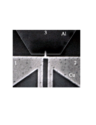
Figure 6: Micrograph of the sample. The sample is made of three arms of Cu wire joining the two Cu reservoirs ”1” and ”2” and one Al superconducting island ”3”. Each arm is 200 nm long, 80 nm wide and 50 nm thick. The voltage probes of the two Cu reservoirs are visible. The Al island is also connected to two measurement probes. For clearity, a thin white line has been drawn around of the Al island. Transport measurement were carried out both between the two Cu reservoirs (”N-n-N” geometry) and between one Cu reservoir and the Al island (N-n-S geometry).

Fig. 6 shows the micrograph of the sample we designed for measuring the re-entrance effect. Preliminary results from this sample were previously published in Ref.[37]. This T-shaped sample is made of three Cu arms joining three wide banks : two are made of Cu, one is of Al. The Al island is superconducting below about $T_{c}=1.3\,K$. The Cu-Al interface has been carefully prepared in view of obtaining a highly transparent interface. From the fit to the theory (see below), we derived a maximum resistance value of $2\,\Omega$ for the N-S interface of area about $200X80\,nm^{2}$. This corresponds to a length $L_{t}$ of about $80\,nm$, which is of the order of the length of the overlapping region between the Cu and Al layers.

The conductance can be measured between the two Cu reservoirs (”N-n-N”) or between one Cu reservoir and the Al island (”N-n-S”). With the first geometry, the redistribution of current paths in the vicinity of the N-S interface[38] due to the superconductivity of Al has a reduced effect on the measured conductance. The normal-state conductance measured between the two Cu reservoirs is $G_{12,N}=0.099\,S$. This gives a mean free path $l_{e}$ of $6\,nm$ and a diffusion coefficient $D=v_{F}l_{e}/3=30\,cm^{2}/s$, using $\rho l_{e}=1.57\,10^{6}\,m.s^{-1}$ for Cu. From this data, we can calculate a value for the Thouless energy $\epsilon_{c}=12\,\mu eV$ associated with the Cu wire length between the two Cu reservoirs. This value is much smaller than the gap $\Delta\simeq 190\,\mu eV$ of Al.

The normal-state conductances of the left (labeled 1) and right (2) arm were measured to be $G_{1N}=0.190\,S$ and $G_{2N}=0.206\,S$ respectively. The conductance of the upper arm in direct contact with the Al island could not be measured directly since the voltage probe was not in close vicinity of the N-S interface. From the fit of the experimental results to the theory, we infer a value $G_{3N}=0.183\,S$ which is compatible with the sample geometry. In the following, all the transport measurements were carried out with an ac bias current corresponding to a voltage modulation of $2\,\mu eV$. This results in a temperature smearing of $23\,mK$.

3.2 The transport measurements

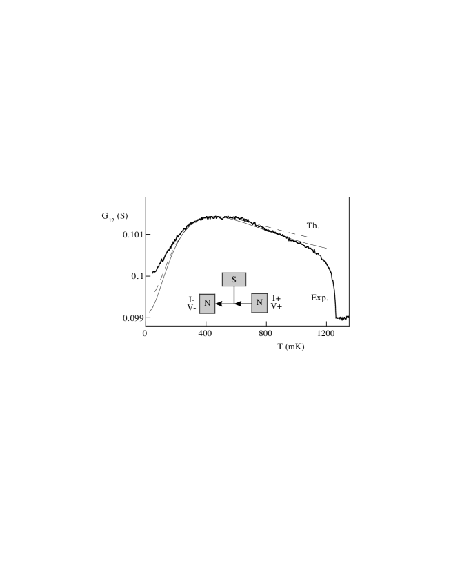
Figure 7: Temperature dependence of the ”N-n-N” sample conductance $G_{12}$ measured between the two N reservoirs at zero bias. The experimental curve (Exp.) is shown in parallel with two theoretical curves (Th.) calculated with the non-linear Usadel equations. The dotted line has been calculated with the assumption of an infinite gap in S and the nominal $\epsilon_{c}=12\,\mu eV$. The full line is with $\epsilon_{c}=15.5\,\mu eV$ and takes into account a constant value for the gap in the Al superconducting island. The phase-breaking length is considered as infinite and the interface transparency is taken as equal to 1.

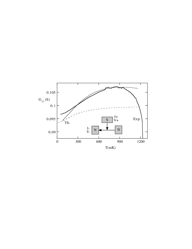
Figure 8: Temperature dependence of the ”N-n-S” sample conductance $G_{13}$ measured between one Cu reservoir and the Al island. Same experimental conditions and fit parameters than previous Figure.

Fig. 7 shows the temperature dependence of the ”N-n-N” conductance $G_{12}$. As the temperature decreases below the superconducting transition of Al, the conductance first rises. It afterwards reaches a maximum near $T=450\,mK$ and eventually decreases down to the lowest temperature ($40\,mK$). This behaviour is characteristic of the re-entrance effect. Here, the conductance decrease amplitude is comparable to the amplitude of the conductance increase at higher energy. Nevertheless, the low-temperature limit of the conductance is significantly higher than the normal-state conductance.

The ”N-n-S” conductance $G_{13}$ measured between the Cu reservoir 1 and the Al island is shown in Fig. 8. The behaviour is qualitatively similar but with quantitative differences. The conductance enhancement is about $10\%$ between $1.2\,K$ and $40\,mK$, instead of $2.5\%$ for $G_{12}$. In the vicinity of the critical temperature of Al, the conductance drops sharply. This behaviour is difficult to analyze because the voltage drop in Al measured in series is also expected to depend strongly on the temperature.

Figure 9: Voltage dependence of the differential conductance of the same sample in the N-n-N measurement geometry. The theoretical curve labeled (QC Th.) is the result of the calculation assuming perfect Cu reservoirs, i.e. with a electron Fermi distribution at the phonon bath temperature. The curve labeled (QC Th. + res.) includes the additional effect of heating of the reservoirs by the bias current. The fit parameters are the same as in the two previous figures.

The bias dependence of the non-linear ”N-n-N” conductance was measured at $40\,mK$ with an ac modulation of the bias current superposed to a dc current bias. Data shown in Fig. 9 exhibit a behaviour which is very similar to the temperature dependence data, both in energy dependence and amplitude. The differential conductance is minimum at zero bias voltage. It shows a maximum at a finite bias voltage of about $40\,\mu eV$ and eventually a decrease at large bias.

In summary, the conductance of N-S structure is shown to be maximum at finite temperature or bias voltage. These two features bring the proof for the re-entrance of the spectral conductance since both experiments probe the spectral conductance. In the zero bias and variable temperature experiment, energy is driven by the bath temperature ($\epsilon\simeq k_{B}T$). In the very-low-temperature and variable bias experiment, energy is driven by the chemical potential of the reservoirs.

The re-entrance of the metallic conductance in a mesoscopic proximity superconductor has been previously observed in other metallic samples[15, 17] and in semiconductor structures.[18] The reentrance of the magnetoresistance oscillations has also been tracked as a function of the bias voltage in semiconductor-superconductor structures, the semiconductor being a two-dimensional electron gas.[16]

4 DISCUSSION

4.1 The detailed spectral conductances

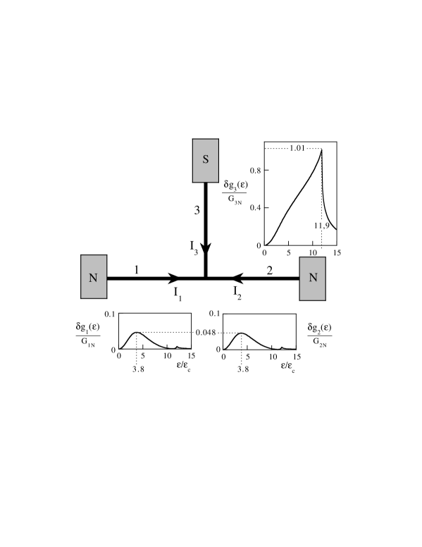
Figure 10: Detail of the calculated spectral conductances of each of three arms constituing the T-shaped sample. The assumed normal-state conductances are $G_{1N}=0.190\,S$, $G_{2N}=0.206\,S$ and $G_{3N}=0.183\,S$. The interface transparency is equal to 1 and the phase-breaking length is considered as infinite. The gap $\Delta$ of S is equal to 12 times the Thouless energy.

We used the quasiclassical theory to quantitatively describe the experimental results. First, the non-linear Usadel equation (Eq. 5) was numerically solved in order to obtain the function $\theta_{2}(x,\epsilon)$. Here we used ideal boundary conditions : $\theta=0$ at the N reservoir, perfect N-S interface with a step-like energy gap (no self-consistency), continuity for $\theta$ and $\delta_{x}\theta$ at the central node. The three spectral conductances $g_{1}(\epsilon)$, $g_{2}(\epsilon)$ and $g_{3}(\epsilon)$ are afterwards derived from the $\theta_{2}$ function.

Fig. 10 shows the three theoretical spectral conductances of the three Cu arms of the sample. The energy unit is the Thouless energy $\epsilon_{c}=\hbar D/L^{2}$ with the length of each branch assumed to be equal to $L/2$. The Thouless energy was taken as a fit parameter. In the following, we will see that the agreement between theory and experiment is better with a Thouless energy of $15.5\,\mu eV$. This value is indeed compatible with our experimental uncertainty on the physical dimensions of the sample. The gap of the superconductor Al is $\Delta\simeq 190\,\mu eV$.

From Fig. 10, the spectral conductances of wires 1 and 2 are maximum at $3.8\,\epsilon_{c}$. The amplitude of the conductance enhancement (here $4.8\,\%$) is significantly smaller than in Fig. 2 because the S island is separated from the wires 1 and 2. A slight local maximum at higher energy is related to the gap of Al. The conductance of the arm 3 is much more affected by the finite amplitude of Al gap. This is because Andreev pairs with an energy close to the gap remain coherent only very close to the N-S interface. The maximum spectral conductance of arm 3 is found slightly below the gap of Al at energy $\epsilon=11\,\epsilon_{c}\simeq\Delta$. The amplitude of this peak ($\delta g_{3}/G_{3N}\simeq 100\%$) is very large. This is remarkable, since the gap of S only appears in the boundary condition at the N-S interface.

4.2 From the spectral conductances to the I-V characteristics

Following Eq. 12, a matrix relation makes the link between the spectral current in each of the three wires and the out-of-equilibrium function $f$ at the nodes of the sample. In our 3-branches circuit, we have :

$$\left\{\begin{array}[]{l}\displaystyle i_{1}=g_{1}\,[f_{1}-f_{N}]\\ i_{2}=g_{2}\,[f_{2}-f_{N}]\\ i_{3}=-g_{3}\,f_{N}\end{array}\right.$$ (19)

where all the quantities are a function of $\epsilon$. Here $f_{1}$, $f_{2}$ and $f_{N}$ are the out-of-equilibrium part $f$ of the energy distribution functions in reservoirs 1, 2 and at the central node. Since the node 3 is the superconducting island, its out-of-equilibrium distribution function $f_{3}$ is zero. The superconducting island 3 is the reference for the voltage. In a N-metal reservoir at voltage $V$ at perfect thermal equilibrium at temperature $T$, $f$ is of the form :[23]

$$f(\epsilon)=\frac{1}{2}[\tanh\{\frac{\epsilon+eV}{2k_{B}T}\}-\tanh\{\frac{\epsilon-eV}{2k_{B}T}\}]$$ (20)

According to the Kirchoff law $i_{1}+i_{2}+i_{3}=0$ at each energy and following Eq. 19, $f_{N}$ is a linear combination of the reservoirs distribution functions :

$$f_{N}=\frac{g_{1}\,f_{1}+g_{2}\,f_{2}}{g_{1}+g_{2}+g_{3}}$$ (21)

where again all the quantities depend on the energy $\epsilon$.

The I-V characteristics were calculated by integration of the equations 19 taken into account the boundary conditions. In the two experimental configurations, they are :

$$\begin{array}[]{lcccc}\displaystyle\mbox{N-n-N}\,\displaystyle:&I_{1}=-I,&I_{2}=I,&I_{3}=0,&V=V_{1}-V_{2}\\ \displaystyle\mbox{N-n-S}\displaystyle\,:&I_{1}=-I,&I_{2}=0,&I_{3}=-I,&V=V_{1}\end{array}$$ (22)

Let us first consider the zero-bias temperature dependence of the conductances. In both Fig. 7 and 8, calculated curves are shown in comparison of the experimental one. Calculated curves are shown in the two cases of an infinite gap taking $\epsilon_{c}=12\,\mu eV$ and with a finite gap $\Delta=12\,\epsilon_{c}=186\,\mu eV$ while $\epsilon_{c}=15.5\,\mu eV$. In the last case, the Thouless energy corresponds to a Thouless temperature $\epsilon_{c}/k_{B}=180\,mK$. The ratio $\Delta/\epsilon_{c}$ is about 12.

The agreement between experiment and theory is satisfactory in the N-n-N geometry in both cases. In the N-n-S geometry, the infinite gap assumption does not provide a good description of the data. The agreement is good in the case of a finite gap and $\epsilon_{c}=15.5\,\mu eV$. The fit is not very accurate near the critical temperature $T_{c}$. This is because our assumption of a constant value for the superconducting gap is not valid anymore in this region.

From these fits, we conclude that the experimental temperature dependence data are well described by the theory. The value of the physical parameters introduced in the calculation are within the measurement uncertainty. The effect of the finite gap is non-negligeable, especially in the N-n-S geometry where the conductance of arm 3 contributes. This is because the pair amplitude $F(\epsilon,x)$ is very large at energies close to the superconductor gap. The Andreev pairs with this value of energy remain coherent only very close to the N-S interface.

At zero energy and zero temperature, one should get the normal-state value of the conductance. This is not seen in the experiment. This may be an effect of the interactions in the normal metal.[25] However, our experiment cannot bring a definitive answer.[32]

Let us now consider the finite bias data. As expected the re-entrance effect, i.e. a conductance peak at energy close to the Thouless energy, is observed in both the calculated and measured data. However, there is no quantitative agreement, as the peak position is at significantly lower energy than expected.

4.3 The role of electron energy distribution in the reservoirs

In order to obtain a better description of the bias dependence experiment, one has to consider the broadening of the energy distribution function in the Cu reservoirs by the injected current. We choose to describe this heating effect by an effective temperature $T_{eff}$ of the reservoir. This effective temperature is different from the phonon temperature and depends on the bias current which is injected in the reservoir.

Two different physical effects may be the cause for a heating of the reservoirs. First, the chemical potential may be ill-defined in the reservoirs. If the reservoir resistance per unit length $\rho_{L}$ is not sufficiently small, a significant potential drop $\rho_{L}L_{in}I$ appears in the reservoir, where $L_{in}$ is the inelastic mean free path. The electron energy distribution will be close to a Fermi distribution with an effective temperature $T_{eff}$. If the inelastic mean free path is temperature-independent, then the effective temperature behaves as $T_{eff}\propto I$.

A second possibility is the Joule effect induced in the reservoirs due to the bias current passing through. This heating power will be evacuated by the phonons. The phonon temperature $T$ will be again different from the effective electron temperature $T_{eff}$. Let us first consider the dissipation due to local Joule heating throughout the sample. The effective temperature then expresses as : $T_{eff}\propto I^{2/5}$ in the limit where $T_{eff}>>T$.[40] In the pure mesoscopic case where the dissipation occurs only in the reservoirs, the Joule effect due to the sample resistance will be evacuated in the reservoirs. The reservoir temperature becomes therefore non-uniform and the diffusion equation for heat has to be solved. Again in the limit where $T_{eff}>>T$, the exponent of the previous power-law will be changed into $4/7$.

The current modulation of the sample creates a modulation of the effective temperature $T_{eff}$. Then, the derivative of the electron energy distribution function writes :

$$\frac{df}{dV}=e\frac{df}{d\epsilon}+\frac{df}{dT_{eff}}\frac{dT_{eff}}{dV}$$ (23)

This introduces an additional term to the usual integration of the spectral conductance over a thermal window, namely a convolution of the spectral conductance with the derivative of a peak function. As a consequence, the usual term of the conductance peak is shifted in the experiment compared to the case of ideal reservoirs.

We described the energy distribution of the electrons in the reservoirs by a Fermi distribution function with a current-dependent effective temperature $T_{eff}$. The effective temperature follows a power law : $T_{eff}=CI^{\alpha}$, with $C$ being a constant common for all the data. We found a better agreement by choosing $\alpha=1$ as compared to the other possible exponents. The ajusted value of the constant $C$ gives an estimate for the inelastic mean free path $L_{in}\simeq 4\mu m$. The result of the calculation is shown in parallel with the experimental curve in Fig. 9. The agreement between experiment and theory is quite improved. The position and amplitude of the conductance peak are well described.

4.4 A direct test of the non-equilibrium distribution function

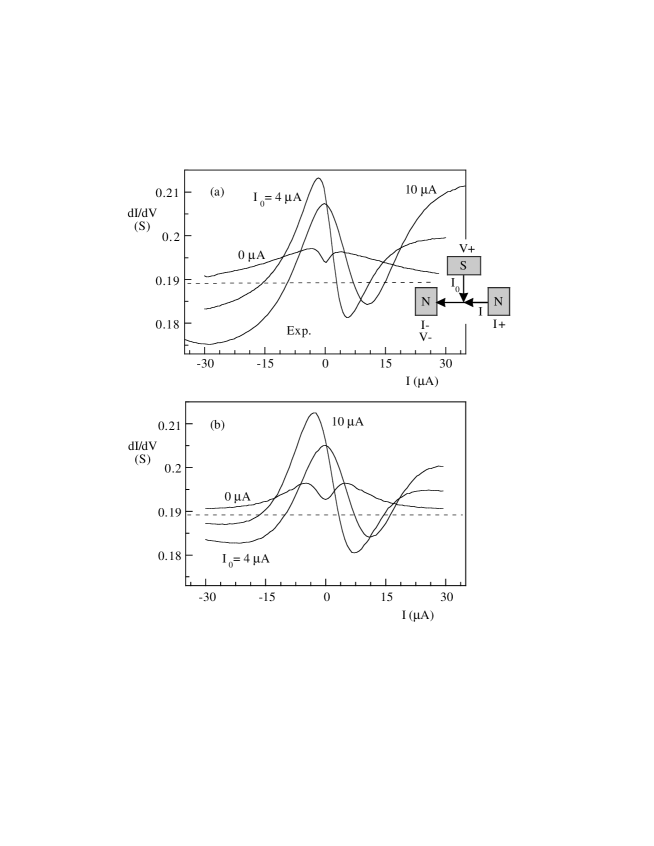
Figure 11: (a) : Measured differential conductance of the left arm of the sample as a function of the bias current for various values of the hot electron injection current $I_{0}$. Temperature is $100\,mK$. (b) : Calculated differential conductance at $T=100\,mK$ of the left arm of the sample as a function of the bias current for various values of the injection current $I_{0}$. In both curves sets, the dashed line indicates the normal-state conductance.

Here we describe a complementary experiment designed to test the assumption of independent energy channels. The strong point is that along the wire, the electron distribution function is strongly non-equilibrium, see e.g. Eq. 21. Indeed, it consists of a superposition of step functions centered at the chemical potential of the respective normal reservoirs. The electron energy distribution has been directly measured in Ref. [39].

The concept is to use the part 3 of the sample as a probe for the distribution function at the node of the sample. The part 3 of the sample has a strongly energy-dependent conductance, like a N-I-S tunnel junction. We injected a dc current $I_{o}$ from the Al probe (3) to the left Cu probe (1) while we measured the resistance of the left arm (1) of Cu. This was made by biasing with a low-frequency ac current between the two Cu probes (1 and 2) and measuring the voltage drop between the Al probe (3) and the left Cu probe (1), see Fig. 11a inset. With a zero injection current, the data show the same behaviour as the full Cu wire, see Fig. 9. With a non-zero injection current, the differential conductance becomes asymmetric in respect of the bias current. Peaks arise, which shift with varying the injection current from $4$ to $10\,\mu A$.

In this configuration, the current in the three branches are $I_{1}=-(I+I_{0})$, $I_{2}=I$, $I_{3}=I_{0}$. As already stressed, the part 3 has the strongest energy dependence of the spectral conductance. For simplicity, our qualitative discussion will neglect the proximity-induced enhancement of the conductance of branches 1 and 2 and keep the contribution of the branch 3 only. We will restrict our qualitative discussion to the zero-temperature limit. By integrating and inverting Eq. 19, we obtain :

$$\left\{\begin{array}[]{l}\displaystyle V_{1}=-\frac{I}{G_{1N}}-[\frac{1}{G_{1N}}+\frac{1}{G_{3N}}]I_{0}+\delta V_{N}\\ \displaystyle V_{2}=\frac{I}{G_{2N}}-\frac{I_{0}}{G_{3N}}+\delta V_{N}\\ \displaystyle V_{N}=-\frac{I_{0}}{G_{3N}}+\delta V_{N}\end{array}\right.$$ (24)

The non-linear contribution $\delta V_{N}$ contains the effect of the energy-dependent conductance enhancement $\delta g_{3}(\epsilon)$ :

$$\delta V_{N}=-\int^{\infty}_{-\infty}{\frac{\delta g_{3}(\epsilon)}{G_{3N}}f_{N}(\epsilon)d\epsilon}$$ (25)

In our experiment, we measure the differential resistance $dV_{1}/dI$ versus $I$ with $I_{0}$ kept constant by an independent floating source. In the normal-state $1/G_{1N}$ is measured. Below $T_{c}$, the non-linear term brings a significant contribution. It measures directly the important features of the distribution function at the central node.

$$\frac{dV_{1}}{dI}|_{I_{0}}=-\frac{1}{G_{1N}}-\int^{\infty}_{-\infty}{\frac{\delta g_{3}(\epsilon)}{G_{3N}}\frac{df_{N}(\epsilon)}{dI}}$$ (26)

At very low temperature, the derivative of the distribution function of the reservoirs $V_{1}$ and $V_{2}$ should tend to $\delta-$functions centered at the chemical potentials of the reservoirs. In this hypothesis, it is straightforward to transform the convolution product into a combination of $\delta g_{3}(eV_{1})$ and $\delta g_{3}(eV_{2})$ using Eq. 21, 19 and 24. The final formula for the conductance $dI/dV$ (here $V=-V_{1}$) is :

$$\frac{dI}{dV_{1}}|_{I_{0}}=G_{1N}[\,1+\frac{G_{1N}}{G_{N}\,G_{3N}}\,\{\delta g_{3}(eV_{2})-\delta g_{3}(eV_{1})\}\,]$$ (27)

with $G_{N}=G_{1N}+G_{2N}+G_{3N}$.

From Eq. 24, we notice that both $V_{1}$ and $V_{2}$ are tuned by the independent driving currents $I$ and $I_{0}$. They vanish respectively for $I^{-}=-I_{0}(1+\,G_{1N}/G_{3N})$ and $I^{+}=I_{0}\,G_{3N}/G_{2N}$. Referring to Fig. 10, the strong minimum of $\delta g_{3}(\epsilon)$ at $\epsilon=0$ show up as a minimum of $\frac{dI}{dV_{1}}$ at $I^{+}$ where $V_{2}=0$ and a maximum at $I^{-}$ where $V_{1}=0$. This is precisely the origin of the strong assymetric behaviour observed in the experimental curve of Fig. 11. The asymmetry is present because of the distribution function $f_{eN}$ at the central node exhibits sharp steps at the chemical potentials of the reservoirs $eV_{1}$ and $eV_{2}$. With this experiment, we have proven that the energy distribution of the electrons at the node in the middle of our sample is truly out-of-equilibrium. In brief, we are indeed in a mesoscopic regime.

In order to achieve a quantitative comparison between theory and experiment, we solved the full matrix expression Eq. 12 which makes no simplification on $\delta g_{1}(\epsilon)$ and $\delta g_{2}(\epsilon)$.We included the heating effect in the reservoirs in the same way than in the re-entrant conductance data. The data of Fig. 11 are well described by using the same constant $C$ and exponent 1 as in the Fig. 7 and 9. As expected, the two extrema occur at values of $I$ proportional to $I_{0}$. When $I_{0}=0$, this contribution is absent. Only the smaller symmetric contribution of $\delta g_{1}(\epsilon)$ remains. Our previous analysis leading to Eq. 27 ignores this contribution but highlights the main contribution due to $\delta g_{3}(\epsilon)$. We also studied an alternate geometry with the inversion of the currents $I$ and $I_{0}$.[32] In this case, the same two terms $\delta g_{3}(eV_{1})$ and $\delta g_{3}(eV_{2})$ are added instead of being subtracted. The experimental data (not shown) were again consistently fitted by the calculation with the same physical parameters.

5 CONCLUSION

In conclusion, we presented a thorough study of the spectral conductance of a mesoscopic normal metal in contact with a superconductor. The spectral conductance exhibits a re-entrance effect at zero energy, i.e. the zero-energy spectral conductance coincides with the normal state conductance. From the theoretical calculations, we observe that the spectral conductance is sensitive to the absolute value of the many physical parameters including : phase-breaking length, gap of the superconductor and interface transparency.

We performed experimental measurement of the reentrance effect as a function of both bias voltage and temperature. The experimental data is well described by the quasiclassical theory. Nevertheless, the description of the non-linear conductance data requires taking into account of the heating of the N reservoirs by the bias current. Compared to a previous study,[17] we were able to describe quantitatively the reentrant resistance with the quasiclassical theory. Thanks to the well-controlled geometry of the normal-metal reservoirs, no scaling factor was necessary.

The large energy-sensitivity of the conductance enhancement by the proximity effect can be used to probe directly the energy distribution function without using a tunnel junction. Thus we were able to measure the conductance enhancement and test the distribution function in a single sample. The whole set of data agree with the theoretically-calculated curves with a single set of physical parameters. This confirms that most of the behaviour of this sample is understood by the theory of the proximity effect in a non-interacting metal. In contrast, the difference between the conductance measured in the zero-temperature limit and the normal-state value raises the question of the importance of the effect of interactions.

We thank F. W. J. Hekking, T. Martin, B. Spivak, A. F. Volkov and F. Zhou for fruitful discussions. This work was supported by the DRET, the Région Rhône-Alpes and the TMR contract ”Dynamics of superconducting nanocircuits” from EU.

References

- [1] C. J. Lambert and R. Raimondi, J. Phys.: Condens. Matter 10, 901 (1998) and references therein.
- [2] D. C. Ralph and V. Ambegaokar, Comments Cond. Mat. 18, 249 (1998).
- [3] D. Estève, in Mesoscopic Electron Transport, Eds. L.P. Kouwenhoven, G. Schön and L.L. Sohn, Kluwer Academic Publishers, Dordrecht, The Netherlands (1996).
- [4] P. Visani, A. C. Mota, A. Pollini, Phys. Rev. Lett. 65, 1514 (1990).
- [5] S. Guéron, H. Pothier, N. O. Birge, D. Estève and M. H. Devoret, Phys. Rev. Lett. 77, 3025 (1996).
- [6] V. T. Petrashov, V. N. Antonov, P. Delsing, and T. Claeson, Phys. Rev. Lett. 70, 347 (1993); Phys. Rev. Lett. 74, 5268 (1995).
- [7] H. Courtois, Ph. Gandit, D. Mailly, and B. Pannetier, Phys. Rev. Lett. 76, 130 (1996).
- [8] V.N. Antonov, A.F. Volkov, and H. Takayanagi, Europhys. Lett. 38, 453 (1997).
- [9] G. E. Blonder, M. Tinkham and T.M. Klapwijk, Phys. Rev. B 25, 4515 (1982).
- [10] A. Kastalsky, A. W. Kleinsasser, L. H. Greene, R. Bhat, F. P. Milliken, and J. P. Harbison, Phys. Rev. Lett. 67, 3026 (1991).
- [11] B.J. van Wees, P. de Vries, P. Magnee and T.M. Klapwijk, Phys. Rev. Lett. 69, 510 (1992).
- [12] F .W. J. Hekking and Y. Nazarov, Phys. Rev. Lett. 71, 1625 (1993); Phys. Rev. B 71, 6847 (1994).
- [13] C. Lambert, J. Phys. Condens. Matter 3, 6579 (1991).
- [14] C. W. J. Beenakker, Phys. Rev. B 46, 12841 (1992).
- [15] P. Charlat, H. Courtois, Ph. Gandit, D. Mailly, A. Volkov, and B. Pannetier, Phys. Rev. Lett. 79, 4950 (1996).
- [16] S. G. den Hartog, C. M. A. Kapteyn, B. J. van Wees, and T. M. Klapwijk, Phys. Rev. Lett. 76, 4592 (1996).
- [17] V. T. Petrashov, R. Sh. Shaikhaidorov, P. Delsing, and T. Claeson, JETP Lett. 67, 513 (1998).
- [18] W. Poirier, D. Mailly, and M. Sanquer, Phys. Rev. Lett. 79, 2105 (1997).
- [19] A. F. Andreev, Sov. Phys. JETP 19, 1228 (1964).
- [20] H. A. Blom, A. Kadigrobov, A. M. Zagoskin, R. I. Shekhter, and M. Jonson, Phys. Rev. B 57, 9995 (1998).
- [21] G. Deutscher and P.G. de Gennes, in Superconductivity, Vol. 2, R.D. Parks, ed. Marcel Dekker, New York (1969).
- [22] A. I. Larkin and Yu. N. Ovchinikov, Sov. Phys. JETP 28, 1200 (1969).
- [23] A. F. Volkov, A. V. Zaitsev, and T. M. Klapwijk, Physica C 210, 21 (1993); A. F. Volkov and A. V. Zaitsev, Phys. Rev. B 53, 9267 (1996); A. V. Zaitsev, JETP Lett. 51, 35 (1990).
- [24] F. Zhou, B. Spivak, and A. Zyuzin, Phys. Rev. B 52, 4467 (1995).
- [25] Y. V. Nazarov and T. H. Stoof, Phys. Rev. Lett. 76, 823 (1996).
- [26] A. A. Golubov, F. K. Wilhelm, and A. D. Zaikin, Phys. Rev. B 55, 1123 (1997).
- [27] S. Yip, Phys. Rev. B 52, 15504 (1995).
- [28] A. F. Volkov, N. Allsopp and C. J. Lambert, J. Phys. Condens. Matter 8, L45 (1996).
- [29] F. Sols and J. Ferrer, Phys. Rev. B 49, 15913 (1994).
- [30] P. Bagwell, Phys. Rev. B 49, 6841 (1994).
- [31] G. B. Lesovik, A. L. Fauchère, and G. Blatter, Phys. Rev. B 55, 3146 (1997)
- [32] P. Charlat, PhD Thesis, University Joseph Fourier, Grenoble (1997).
- [33] M. Giroud, H. Courtois, K. Hasselbach, D. Mailly, and B. Pannetier, Phys. Rev. B 58, R11872 (1998).
- [34] B. Pannetier, J. Chaussy, and R. Rammal, Phys. Scripta T 13, 245, (1986).
- [35] H. Pothier, S. Guéron, D. Estève, and M. H. Devoret, Phys. Rev. Lett. 73, 2488 (1994).
- [36] A. F. Volkov, V. V. Pavlovskii, and R. Seviour, to appear in Sup. and Microstructures.
- [37] P. Charlat, H. Courtois, Ph. Gandit, D. Mailly, A. Volkov, and B. Pannetier, Proceedings of the LT21 Conference, Czech. J. of Phys. 46, S6 3107 (1996).
- [38] F. K. Wilhelm, A. D. Zaikin and H. Courtois, Phys. Rev. Lett. 80, 4289 (1998).
- [39] H. Pothier, S. Guéron, N. O. Birge, D. Esteve, and M. H. Devoret, Phys. Rev. Lett. 79, 3490 (1997).
- [40] M. L. Roukes, M. R. Freeman, R. S. Germain, R. C. Richardson and M. B. Ketchen, Phys. Rev. Lett. 55, 422 (1985).