Kinetic theory of shot noise in non-degenerate diffusive conductors

Abstract

We investigate current fluctuations in non-degenerate semiconductors, on length scales intermediate between the elastic and inelastic mean free paths. We present an exact solution of the non-linear kinetic equations in the regime of space-charge limited conduction, without resorting to the drift approximation of previous work. By including the effects of a finite voltage and carrier density in the contact region, a quantitative agreement is obtained with Monte Carlo simulations by González et al., for a model of an energy-independent elastic scattering rate. The shot-noise power $P$ is suppressed below the Poisson value $P_{\rm Poisson}=2e\bar{I}$ (at mean current $\bar{I}$) by the Coulomb repulsion of the carriers. The exact suppression factor is close to $1/3$ in a three-dimensional system, in agreement with the simulations and with the drift approximation. Including an energy dependence of the scattering rate has a small effect on the suppression factor for the case of short-range scattering by uncharged impurities or quasi-elastic scattering by acoustic phonons. Long-range scattering by charged impurities remains an open problem.

I Introduction

The kinetic theory of non-equilibrium fluctuations in an electron gas was pioneered by Kadomtsev in 1957 [1] and fully developed ten years later [2, 3]. The theory has been comprehensively reviewed by Kogan [4]. In recent years there has been a revival of the interest in this field, because of the discovery of fundamental effects on the mesoscopic length scale. (See Ref. [5] for a recent review.) One of these effects is the sub-Poissonian shot noise in degenerate electron gases on length scales intermediate between the mean free path $\ell$ for elastic impurity scattering and the inelastic mean free path $\ell_{\rm in}$ for electron-phonon or electron-electron scattering. The universal one-third suppression of the shot-noise power predicted theoretically [6, 7] has been observed in experiments on semiconductor or metal wires of micrometer length [8, 9, 10, 11].

The electron density in these experiments is sufficiently high that the electron gas is degenerate. The reduction of the shot-noise power

$$P=2\int_{-\infty}^{\infty}{\rm d}t^{\prime}\,\overline{\delta I(t)\delta I(t+t^{\prime})}$$ (1)

[with $\delta I(t)$ the fluctuations of the current around the mean current $\bar{I}$] below the Poisson value $P_{\rm Poisson}=2e\bar{I}$ is then the result of correlations induced by the Pauli exclusion principle. When the electron density is reduced, the Pauli principle becomes ineffective. One enters then the regime of a non-degenerate electron gas, studied recently in Monte Carlo simulations by González et al. [12]. In a model of energy-independent three-dimensional elastic impurity scattering these authors found the very same ratio $P/P_{\rm Poisson}=1/3$ as in the degenerate case. The origin of the suppression is quite different, however, being due to correlations induced by long-range Coulomb repulsion — rather than by the Pauli principle. The one-third suppression of shot-noise in the computer simulations required a large voltage and short screening length, but was found to be otherwise independent of material parameters.

Subsequent analytical work by one of the authors [13] explained this universality as a feature of the regime of space-charge limited conduction. The kinetic equations in this regime are highly non-linear, and could only be solved in the approximation that the diffusion term is neglected compared to the drift term. This is a questionable approximation: The ratio of the two terms is $1/d$, with $d$ the dimensionality of the density of states. The result of Ref. [13],

$$P/P_{\rm Poisson}=\frac{12}{5}\frac{3d^{2}+22d+64}{(d+2)(3d+4)(3d+8)},$$ (2)

becomes exact in the large-$d$ limit, when $P/P_{\rm Poisson}\to 4/5d$, but has an error of unknown magnitude for the physically relevant value $d=3$.

The main purpose of the present paper is to report the exact solution of the kinetic equations in the space-charge limited transport regime. We find that inclusion of the diffusion term has a pronounced effect on the spatial dependence of the electric field, although the ultimate effect on the noise power turns out to be relatively small: The exact suppression factor differs from Eq. (2) by about $10\%$ for $d=3$. We find

$$P/P_{\rm Poisson}=\left\{\begin{array}[]{cc}0.6857&\quad\mbox{for}\quad d=1,\\ 0.4440&\quad\mbox{for}\quad d=2,\\ 0.3097&\quad\mbox{for}\quad d=3,\end{array}\right.$$ (3)

close to the values reported by González et al. (although their surmise that $P/P_{\rm Poisson}$ is a simple fraction $1/d$ for $d=2$, $3$ is not borne out by this exact calculation). By including the effects of a finite temperature and screening length, we obtain excellent agreement with the electric field profiles in the simulations (which could not be achieved in the drift approximation of Ref. [13]), and determine the conditions for space-charge limited conduction. We also go beyond previous work by calculating to what extent the shot-noise suppression factor varies with the energy-dependence of the scattering rate. (This breakdown of universality was anticipated in Refs. [13] and [14].)

The paper is organized as follows. The kinetic theory is introduced in Sec. II, where we summarize the basic equations and emphasize the differences with the degenerate case. In Sec. III we formulate the problem for the regime of space-charge limited conduction. In Sec. IV we solve the kinetic equations for the case of an energy-independent scattering rate and compare with the Monte Carlo simulations [12]. We study separately the capacitance fluctuations. The effect of deviations from the conditions of space-charge limited conduction is also investigated. Energy-dependence in the scattering rate is considered in Sec. V. We conclude in Sec. VI with a discussion of the experimental observability in connection with electron-phonon scattering.

II Kinetic theory

A Boltzmann-Langevin equation

Our starting point is the same kinetic theory [1, 2, 3, 4] used to study shot noise in degenerate conductors [5, 7, 15, 16, 17, 18, 19, 20, 21]. We summarize the basic equations, emphasizing the differences in the non-degenerate case. The density $f({\bf r},{\bf p},t)$ of carriers at position ${\bf r}$ and momentum ${\bf p}=m{\bf v}$ at time $t$ (where $m$ is the effective mass and v the velocity) satisfies the Boltzmann-Langevin equation

$$\left[\frac{\partial}{\partial t}+{\bf v}\cdot\frac{\partial}{\partial\bf r}+e{\bf E}({\bf r},t)\cdot\frac{\partial}{\partial\bf p}\right]f({\bf r},{\bf p},t)={\cal S}+\delta J.$$ (4)

Here ${\bf E}({\bf r},t)$ is the electric field (we take the charge of the carriers positive), ${\cal S}({\bf r},{\bf p},t)$ is the collision integral, and $\delta J({\bf r},{\bf p},t)$ is a fluctuating source (or “Langevin current”). The collision integral describes the average effect of elastic impurity scattering,

$${\cal S}({\bf r},p{\bf\hat{n}},t)$$ (6)

$$\quad=\int\frac{{\rm d}{\bf\hat{n}}^{\prime}}{\Omega}W_{\varepsilon}({\bf\hat{n}}\cdot{\bf\hat{n}}^{\prime})[f({\bf r},p{\bf{\hat{n}}}^{\prime},t)-f({\bf r},p{\bf\hat{n}},t)].$$

The integral over the direction ${\bf\hat{n}}={\bf p}/p$ of the momentum extends over the surface of the unit sphere in $d$ dimensions, with surface area $\Omega=2\pi^{d/2}/\Gamma(\frac{1}{2}d)$. The scattering rate $W_{\varepsilon}({\bf\hat{n}}\cdot{\bf\hat{n}}^{\prime})$ depends on the kinetic energy $\varepsilon=p^{2}/2m$ and on the scattering angle ${\bf\hat{n}}\cdot{\bf\hat{n}}^{\prime}$. The effective mass $m$ is assumed to be energy independent.

The stochastic Langevin current $\delta J$ vanishes on average, $\overline{\delta J}=0$, and has correlator [2]

$$\overline{\delta J({\bf r},{\bf p},t)\delta J({\bf r}^{\prime},{\bf p}^{\prime},t^{\prime})}=\delta({\bf r}-{\bf r}^{\prime})\delta(t-t^{\prime})\delta(\varepsilon-\varepsilon^{\prime})\frac{1}{\nu(\varepsilon)}$$ (7)

$$\quad{}\times\Big{[}\delta({\bf\hat{n}}-{\bf\hat{n}}^{\prime})\int{\rm d}{\bf\hat{n}}^{\prime\prime}\,W_{\varepsilon}({\bf\hat{n}}\cdot{\bf\hat{n}}^{\prime\prime})(\bar{f}+\bar{f}^{\prime\prime}-2\bar{f}\bar{f}^{\prime\prime})$$ (8)

$$\quad\qquad{}-W_{\varepsilon}({\bf\hat{n}}\cdot{\bf\hat{n}}^{\prime})(\bar{f}+\bar{f}^{\prime}-2\bar{f}\bar{f}^{\prime})\Big{]},$$ (9)

determined by the mean occupation number ${\bar{f}}$. (We abbreviated $\bar{f}^{\prime}=\bar{f}({\bf r},{\bf p}^{\prime},t)$ and analogously for $\bar{f}^{\prime\prime}$.) The density of states in $d$ dimensions is $\nu(\varepsilon)=m\Omega(2m\varepsilon)^{d/2-1}$, where we set Planck’s constant $h\equiv 1$.

A non-degenerate electron gas is characterized by ${\bar{f}}\ll 1$. In contrast to the degenerate case, the Pauli exclusion principle is then of no effect. One consequence is that we may omit the terms quadratic in ${\bar{f}}$ in the correlator (9). A second consequence is that deviations from equilibrium are no longer restricted to a narrow energy range around the Fermi level, but extend over a broad range of $\varepsilon$. One can not, therefore, eliminate $\varepsilon$ as an independent variable from the outset, as in the degenerate case.

B Diffusion approximation

We assume that the elastic mean free path is short compared to the dimensions of the conductor, so that we can make the diffusion approximation. This consists in keeping only the two leading terms,

$$f({\bf r},{\bf\hat{n}}\sqrt{2m\varepsilon},t)={\cal F}({\bf r},\varepsilon,t)+{\bf\hat{n}}\cdot{\bf f}({\bf r},\varepsilon,t),$$ (10)

of a multipole expansion in the momentum direction $\bf\hat{n}$. We substitute Eq. (10) into the Boltzmann-Langevin equation (4) and integrate over ${\bf\hat{n}}$ to obtain the continuity equation,

$$\frac{\partial}{\partial t}\rho({\bf r},\varepsilon,t)+\frac{\partial}{\partial{\bf r}}\cdot{\bf j}({\bf r},\varepsilon,t)+e{\bf E}({\bf r},t)\cdot\frac{\partial}{\partial\varepsilon}{\bf j}({\bf r},\varepsilon,t)=0,$$ (11)

for the energy-resolved charge and current densities

$$\rho({\bf r},\varepsilon,t) = e\nu(\varepsilon){\cal F}({\bf r},\varepsilon,t),$$ (12)

$${\bf j}({\bf r},\varepsilon,t) = \frac{1}{d}ev\nu(\varepsilon){\bf f}({\bf r},\varepsilon,t),$$ (13)

with $v=\sqrt{2\varepsilon/m}$. In the zero-frequency limit we may omit the time derivative in Eq. (11).

Multiplication by ${\bf\hat{n}}$ followed by integration gives a second relation between $\rho$ and ${\bf j}$ [22],

$${\bf j}({\bf r},\varepsilon,t) = -D(\varepsilon)\frac{\partial}{\partial{\bf r}}\rho({\bf r},\varepsilon,t)$$ (15)

$${}-\sigma(\varepsilon){\bf E}({\bf r},t)\frac{\partial}{\partial\varepsilon}{\cal F}({\bf r},\varepsilon,t)+\delta{\bf J}({\bf r},\varepsilon,t),$$

a combination of Fick’s law and Ohm’s law with a fluctuating current source. The conductivity $\sigma(\varepsilon)=e^{2}\nu(\varepsilon)D(\varepsilon)$ is the product of the density of states and the diffusion constant $D(\varepsilon)=v^{2}\tau/d=(2\varepsilon/md)\tau(\varepsilon)$. The scattering rate is given by

$$\frac{1}{\tau(\varepsilon)}=\int\frac{{\rm d}{\bf\hat{n}}^{\prime}}{\Omega}W_{\varepsilon}({\bf\hat{n}}\cdot{\bf\hat{n}}^{\prime})(1-{\bf\hat{n}}\cdot{\bf\hat{n}}^{\prime}).$$ (16)

The energy-resolved Langevin current

$$\delta{\bf J}({\bf r},\varepsilon,t)=e\tau(\varepsilon)v\nu(\varepsilon)\int\frac{{\rm d}{\bf\hat{n}}}{\Omega}{\bf\hat{n}}\,\delta J({\bf r},{\bf\hat{n}}\sqrt{2m\varepsilon},t)$$ (17)

is correlated as

$$\overline{\delta J_{l}({\bf r},\varepsilon,t)\delta J_{m}({\bf r}^{\prime},\varepsilon^{\prime},t^{\prime})}$$ (19)

$${}=2\sigma(\varepsilon)\bar{\cal F}({\bf r},\varepsilon,t)\delta_{lm}\delta({\bf r}-{\bf r}^{\prime})\delta(t-t^{\prime})\delta(\varepsilon-\varepsilon^{\prime}),$$

where we have omitted terms quadratic in $\bar{\cal F}$.

These kinetic equations should be solved together with the Poisson equation

$$\kappa\frac{\partial}{\partial{\bf r}}\cdot{\bf E}({\bf r},t)=\rho({\bf r},t)-\rho_{\rm eq},$$ (20)

with $\rho({\bf r},t)=\int{\rm d}\varepsilon\,\rho({\bf r},\varepsilon,t)$ the integrated charge density, $\kappa$ the dielectric constant, and $\rho_{\rm eq}$ the mean charge density in equilibrium. The Langevin current $\delta J$ induces fluctuations in $\rho$ and hence in $\bf E$. The need to take the fluctuations in the electric field into account selfconsistently is a severe complication of the problem.

C Slab geometry

We consider the slab geometry of Fig. 1, consisting of a semiconductor aligned along the $x$-axis with uniform cross-sectional area $A$. A non-fluctuating potential difference $V$ is maintained between the metal contacts at $x=0$ and $x=L$, with the current source at $x=0$. The contacts are in equilibrium at temperature $T$. It is convenient to integrate over energy and the coordinates ${\bf r}_{\perp}$ perpendicular to the $x$-axis. We define the linear charge density $\rho(x,t)=\int{\rm d}{\bf r}_{\perp}\,\rho({\bf r},t)$ and the currents $I(t)=\int{\rm d}{\bf r}_{\perp}\,\int{\rm d}\varepsilon\,j_{x}({\bf r},\varepsilon,t)$ and $\delta J(x,t)=\int{\rm d}{\bf r}_{\perp}\,\int{\rm d}\varepsilon\,\delta J_{x}({\bf r},\varepsilon,t)$. The current $I$ is $x$-independent in the zero-frequency limit because of the continuity equation (11). We also define the electric field profile $E(x,t)=A^{-1}\int{\rm d}{\bf r}_{\perp}\,E_{x}({\bf r},t)$. The vector ${\bf r}_{\perp}$ of transverse coordinates has $d-1$ dimensions. The physically relevant case is $d=3$, but in computer simulations one can consider other values of $d$. For example, in Ref. [12] the case $d=2$ was also studied, corresponding to a hypothetical “Flatland” [23]. To compare with the simulations, we will also consider arbitrary $d$.

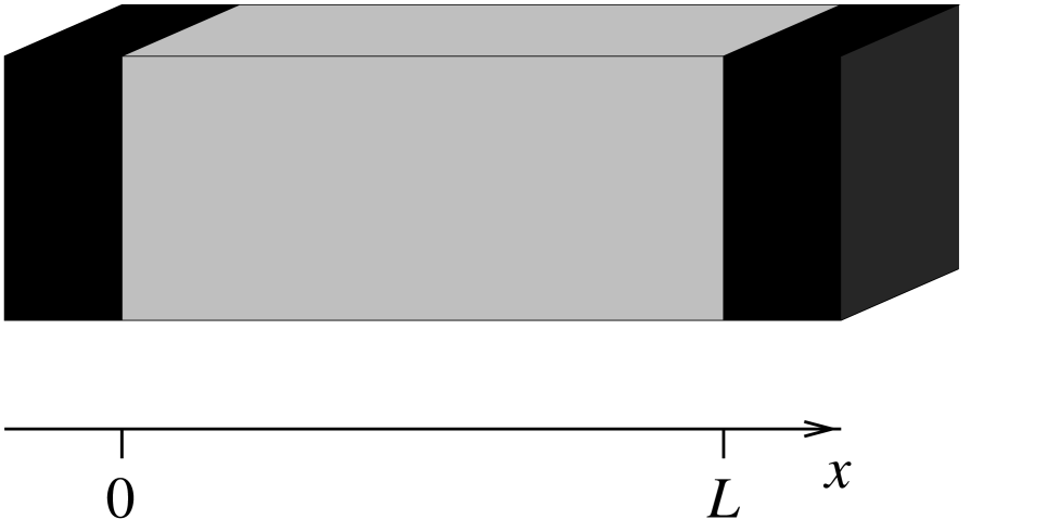
FIG. 1.: Semiconducting slab (grey) between two metal contacts (black) at $x=0$ and $x=L$. The $(d-1)$-dimensional cross-sectional area is $A$. The current flows from left to right in response to a voltage $V$ applied between the contacts.

For any $d$ the fluctuating Ohm-Fick law (15) takes the one-dimensional form

$$I(t) = -\frac{\partial}{\partial x}\int{\rm d}{\bf r}_{\perp}\int{\rm d}\varepsilon\,D(\varepsilon)\rho({\bf r},\varepsilon,t)$$ (23)

$${}+E(x,t)\int{\rm d}{\bf r}_{\perp}\int{\rm d}\varepsilon\,{\cal F}({\bf r},\varepsilon,t)\frac{\rm d}{{\rm d}\varepsilon}\sigma(\varepsilon)$$

$${}+\delta J(x,t),$$

where we used that the averages of $\cal F$ and ${\bf E}$ depend on $x$ only and neglected terms quadratic in the fluctuations. The Poisson equation (20) becomes

$$\kappa A\frac{\partial}{\partial x}E(x,t)=\rho(x,t)-A\rho_{\rm eq},$$ (24)

and the correlator (19) becomes

$$\overline{\delta{J}(x,t)\delta{J}(x^{\prime},t^{\prime})}$$ (26)

$$\quad=2A\delta(t-t^{\prime})\delta(x-x^{\prime})\int{\rm d}\varepsilon\,\sigma(\varepsilon)\bar{\cal F}(x,\varepsilon).$$

Our problem is to compute from Eqs. (23) – (26) the shot-noise power (1).

D Energy-independent scattering time

The Ohm-Fick law (23) simplifies in the model of an energy-independent scattering time $\tau(\varepsilon)\equiv\tau$. Then the derivative of the conductivity ${\rm d}\sigma/{\rm d}\varepsilon=e\mu\,\nu(\varepsilon)$ is proportional to the density of states, and contains the energy-independent mobility $\mu=e\tau/m$. Eq. (23) becomes

$$I(t) = -\frac{\partial}{\partial x}\int{\rm d}{\bf r}_{\perp}\int{\rm d}\varepsilon\,D(\varepsilon)\rho({\bf r},\varepsilon,t)$$ (28)

$${}+\mu\,\rho(x,t)E(x,t)+\delta J(x,t).$$

The drift term has now the same form $\mu\rho E$ as for inelastic scattering [24]. This simple form does not hold for the more general case of energy-dependent elastic scattering.

III Space-charge limited conduction

For a large voltage drop $V$ between the two metal contacts and a high carrier density $\rho_{c}$ in the contacts, the charge injected into the semiconductor is much higher than the equilibrium charge $\rho_{\rm eq}$, which can then be neglected. For sufficiently high $V$ and $\rho_{c}$ the system enters the regime of space-charge limited conduction [25], defined by the boundary condition

$$E(x,t)=0\quad\mbox{at}\quad x=0.$$ (29)

Eq. (29) states that the space charge $Q=\int_{0}^{L}\rho(x)\,{\rm d}x$ in the semiconductor is precisely balanced by the surface charge at the current drain. The accuracy of this boundary condition at finite $V$ and $\rho_{c}$ is examined in Sec. IV E. At the drain we have the absorbing boundary condition

$$\rho(x,t)=0\quad\mbox{at}\quad x=L.$$ (30)

With this boundary condition we again neglect $\rho_{\rm eq}$.

To determine the electric field inside the semiconductor we proceed as follows. The potential gain $-e\phi(x,t)$ (with $E=-\partial\phi/\partial x$) dominates over the initial thermal excitation energy of order $kT$ (with Boltzmann’s constant $k$) almost throughout the whole semiconductor; only close to the current source (in a thin boundary layer) this is not the case. We can therefore approximate the kinetic energy $\varepsilon\approx-e\phi$ and introduce this into $D(\varepsilon)$ and ${\rm d}\sigma/{\rm d}\varepsilon$. We assume a power-law energy dependence of the scattering time $\tau=\tau_{0}\varepsilon^{\alpha}$. Then $D(\varepsilon)=(2\tau_{0}/md)\varepsilon^{\alpha+1}\approx-(2\mu_{0}/d)(-e)^{\alpha}\phi^{\alpha+1}$ and ${\rm d}\sigma/{\rm d}\varepsilon=(2\alpha+d)(\tau_{0}/md)e^{2}\varepsilon^{\alpha}\nu(\varepsilon)\approx-(2\alpha+d)(\mu_{0}/d)(-e)^{\alpha+1}\phi^{\alpha}\nu(\varepsilon)$, where we have defined $\mu_{0}=e\tau_{0}/m$. Substituting into Eq. (23) and using the Poisson equation $-\kappa A{\partial^{2}}\phi/\partial x^{2}=\rho$ we find the third-order, non-linear, inhomogeneous differential equation

$$(2\alpha+d)\phi^{\alpha}\frac{\partial}{\partial x}\left(\frac{\partial\phi}{\partial x}\right)^{2}-4\frac{\partial}{\partial x}\left(\phi^{\alpha+1}\frac{\partial^{2}\phi}{\partial x^{2}}\right)$$ (31)

$$\qquad=\frac{2d}{(-e)^{\alpha}\mu_{0}\kappa A}[I(t)-\delta{J}(x,t)]$$ (32)

for the potential profile $\phi(x,t)$.

Since the potential difference $V$ between source and drain does not fluctuate, we have the two boundary conditions

$$\phi(x,t)= 0~{}~{} \quad\mbox{at}\quad x=0,$$ (33)

$$\phi(x,t)= -\!V \quad\mbox{at}\quad x=L.$$ (34)

Eqs. (29) and (30) imply two additional boundary conditions,

$$\frac{\partial}{\partial x}\phi(x,t)=0 \quad x=0,$$ at (35)

$$\frac{\partial^{2}}{\partial x^{2}}\phi(x,t)=0 \quad x=L.$$ at (36)

We will now solve this boundary value problem for $\phi=\bar{\phi}+\delta\phi$, first for the mean and then for the fluctuations, in both cases neglecting terms quadratic in $\delta\phi$. The case $\alpha=0$ of an energy-independent scattering time is considered first, in Sec. IV. The more complicated case of non-zero $\alpha$ is treated in Sec. V.

IV Energy-independent scattering time

A Average profiles

For $\alpha=0$ the averaged equation (32) can be integrated once to obtain the second-order differential equation

$$\left(\frac{{\rm d}\bar{\phi}}{{\rm d}x}\right)^{2}-\frac{4}{d}\bar{\phi}\frac{{\rm d}^{2}\bar{\phi}}{{\rm d}x^{2}}=\frac{2\bar{I}}{\mu\kappa A}x$$ (37)

for the mean potential $\bar{\phi}(x)$. In this case of an energy-independent scattering time $\tau(\varepsilon)\equiv\tau$ we may identify $\mu_{0}$ with the mobility $\mu=e\tau/m$ introduced in Sec. II D. No integration constant appears in Eq. (37), since only then the boundary conditions (33) and (35) at $x=0$ can be fulfilled simultaneously. In Ref. [13] the second term on the left-hand-side of Eq. (37) (the diffusion term) was neglected relative to the first term (the drift term). This approximation is rigorously justified only in the formal limit $d\to\infty$. It has the drawback of reducing the order of the equation by one, so that no longer all boundary conditions can be fulfilled. Although the solution in Ref. [13] violates the absorbing boundary condition (36), the final result for the shot-noise power turns out to be close to the exact result obtained here.

Before solving this non-linear differential equation exactly, we discuss two scaling properties that help us along the way. Note first that the current $\bar{I}$ can be scaled away by the substitution

$$\bar{\phi}(x)=-\left(\frac{2\bar{I}}{\mu\kappa A}\right)^{1/2}\chi(x).$$ (38)

Secondly, each solution $\chi(x)$ of

$$\left(\frac{{\rm d}\chi}{{\rm d}x}\right)^{2}-\frac{4}{d}\chi\frac{{\rm d}^{2}\chi}{{\rm d}x^{2}}=x$$ (39)

[the rescaled Eq. (37)] generates a one-parameter family of solutions $\lambda^{3/2}\chi(x/\lambda)$. Thus, if we find a solution which fulfills the three boundary conditions $\chi(0)=0$, $\chi^{\prime}(0)=0$, $\chi^{\prime\prime}(1)=0$ (primes denoting differentiation with respect to $x$), then the potential

$$\bar{\phi}(x)=-\left(\frac{2\bar{I}L^{3}}{\mu\kappa A}\right)^{1/2}\chi(x/L)$$ (40)

solves Eq. (37) with boundary conditions (33), (35), and (36). The remaining boundary condition (34) determines the current-voltage characteristic

$$\bar{I}(V)=\frac{\mu\kappa A}{2L^{3}}\left(\frac{V}{\chi(1)}\right)^{2}.$$ (41)

The quadratic dependence of $\bar{I}$ on $V$ is the Mott-Gurney law of space-charge limited conduction [26].

We now construct a solution $\chi(x)$. One obvious solution is $\chi_{0}(x)=a_{0}x^{3/2}$, with

$$a_{0}=\frac{2}{3}\left(1-\frac{4}{3d}\right)^{-1/2}.$$ (42)

This solution satisfies the boundary conditions at $x=0$, but $\chi^{\prime\prime}_{0}(x)\neq 0$ for any finite $x$. Close to the singular point $x=0$ any solution will approach $\chi_{0}(x)$ provided that $d>4/3$. Let us discuss first this range of $d$, containing the physically relevant dimension $d=3$.

We substitute into Eq. (39) the ansatz

$$\chi(x)=\sum_{l=0}^{\infty}a_{l}x^{\beta l+3/2},$$ (43)

consisting of $\chi_{0}(x)$ times a power series in $x^{\beta}$, with $\beta$ a positive power to be determined. This ansatz proves fruitful since both terms on the left-hand-side of Eq. (39) give the same powers of $x$, starting with order $x^{1}$ in coincidence with the right-hand-side. Power matching gives Eq. (42) for $a_{0}$ and for $l\geq 1$ the conditions

$$\sum_{m=0}^{l}b_{lm}a_{m}a_{l-m}=0,$$ (44)

$$b_{lm}=\frac{9}{4}-\frac{3}{d}+\left(3-\frac{8}{d}\right)m\beta-\left(1+\frac{4}{d}\right)m^{2}\beta^{2}+ml\beta^{2}.$$ (45)

The relation with $l=1$ is special: It determines the power $\beta$,

$$\beta^{2}+\beta\left(2-\frac{3}{4}d\right)+\frac{3}{2}-\frac{9}{8}d=0,$$ (46)

but leaves the coefficient $a_{1}$ as a free parameter [to be determined by demanding that $\chi^{\prime\prime}(1)=0$]. The positive solution of Eq. (46) is

$$\beta=\frac{3}{8}d-1+\frac{1}{8}\sqrt{9d^{2}+24d-32}.$$ (47)

We find $\beta=(\sqrt{13}-1)/4$ for $d=2$ and $\beta=3/2$ for $d=3$. For $l\geq 2$ we solve for $a_{l}$ to obtain the recursion relation

$$a_{l}=-\frac{\sum_{m=1}^{l-1}b_{lm}a_{m}a_{l-m}}{(b_{ll}+b_{l0})a_{0}}.$$ (48)

FIG. 2.: Profile of the mean electrical potential $\bar{\phi}$ [in units of $(2\bar{I}L^{3}/\mu\kappa A)^{1/2}$], the electric field $\bar{E}$ [in units of $(2\bar{I}L/\mu\kappa A)^{1/2}$], and the charge density $\bar{\rho}$ [in units of $(2\bar{I}\kappa/\mu LA)^{1/2}$], following from Eq. (37) for different values of $d$. The drift approximation of Ref. [13] corresponds to the case $d=\infty$ in this plot.

Interestingly enough, the power series terminates for $d=12/5$, and the solution for this dimension is $\chi(x)=x^{3/2}-\frac{1}{5}x^{5/2}$. For arbitrary dimension $d>4/3$, the coefficients $a_{l}$ fall off with $l$, the more rapidly so the larger $d$. We find numerically that the solution with $\chi^{\prime\prime}(1)=0$ has $a_{1}=0.3261$ for $d=2$ and $a_{1}=0.1166$ for $d=3$.

For $d<4/3$ we substitute into Eq. (39) the ansatz

$$\chi(x)=\sum_{l=0}^{\infty}c_{l}x^{\gamma l+(3-\gamma)/2},$$ (49)

with $\gamma=(4-3d)/(4-d)$. Now the coefficient $c_{0}$ is free. Power matching gives further

$$c_{1}=-\frac{d}{4\gamma(\gamma+1)},$$ (50)

and the recursion relation

$$c_{l}=-\frac{\sum_{m=1}^{l-1}d_{lm}c_{m}c_{l-m}}{(d_{ll}+d_{l0})c_{0}},$$ (51)

$$d_{lm}=\left(\gamma m+\frac{3-\gamma}{2}\right)\left[\gamma(l-m)-\frac{4}{d}\gamma m\right],$$ (52)

for coefficients with $l\geq 2$. For $d=1$ the solution with $\chi^{\prime\prime}(1)=0$ has $c_{0}=1.3628$.

In Fig. 2 the profiles of the potential $\bar{\phi}\propto\chi$, the electric field $\bar{E}\propto\chi^{\prime}$, and the charge density $\bar{\rho}\propto\chi^{\prime\prime}$ are plotted for $d=1$, $2$, $3$. We also show the result for $d=\infty$, corresponding to the drift approximation of Ref. [13]. The coefficient $\chi(1)$ appearing in the current-voltage characteristic (41) can be read off from this plot. We find $\chi(1)=8/9$ for $d=1$, $\chi(1)=0.8180$ for $d=2$, and $\chi(1)=0.7796$ for $d=3$. The limiting value for $d=\infty$ is $\chi(1)=2/3$.

B Fluctuations

For the fluctuations it is again convenient to work with the rescaled mean potential (38). We rescale the fluctuations in the same way,

$$\delta\phi(x,t)=-\left(\frac{2\bar{I}}{\mu\kappa A}\right)^{-1/2}\psi(x,t).$$ (53)

We linearize Eq. (32) with $\alpha=0$ around the mean values and integrate once to obtain the second-order inhomogeneous linear differential equation

$${\cal L}[\psi] = -\left(\frac{4}{d}\chi\right)\frac{{\partial}^{2}\,\psi}{{\partial}x^{2}}+\left(2\frac{{\rm d}\chi}{{\rm d}x}\right)\frac{{\partial}\,\psi}{{\partial}x}-\left(\frac{4}{d}\frac{{\rm d}^{2}\chi}{{\rm d}x^{2}}\right)\psi$$ (54)

$$= \int_{0}^{x}{\rm d}x^{\prime}\,\frac{\delta I(t)-\delta{J}(x^{\prime},t)}{\bar{I}}.$$ (55)

The integration constant vanishes as a consequence of the boundary condition

$$\psi(x,t)=0\quad\mbox{at}\quad x=0$$ (56)

and the requirement that the fluctuating electric field ${\partial\psi}/{\partial x}$ stays finite at $x=0$. [The latter condition actually implies $\partial\psi/{\partial x}=0$ at $x=0$.] We will solve Eq. (55) with the additional condition of a non-fluctuating voltage,

$$\psi(x,t)=0\quad\mbox{at}\quad x=L.$$ (57)

The remaining constraint

$$\frac{\partial^{2}}{\partial x^{2}}\psi(x,t)=0\quad\mbox{at}\quad x=L$$ (58)

(the absorbing boundary condition) will be used later to relate $\delta I$ to $\delta{J}$.

We need the Green function $G(x,x^{\prime})$, satisfying for each $x^{\prime}$ the equation ${\cal L}[G(x,x^{\prime})]=\delta(x-x^{\prime})$. In view of Eq. (39) for the mean potential one recognizes

$$\psi_{1}(x)=3\chi(x)-2x\,\frac{{\rm d}}{{\rm d}x}\chi(x)$$ (59)

as a solution ${\cal L}[\psi_{1}]=0$ which already satisfies Eq. (56). Using a standard prescription [27] we find from $\psi_{1}(x)$ a second, independent, homogeneous solution

$$\psi_{2}(x)=\psi_{1}(x)\int_{x}^{L}\!\!{\rm d}x^{\prime}\,\frac{\chi^{d/2}(x^{\prime})}{\psi_{1}^{2}(x^{\prime})},$$ (60)

which fulfills Eq. (57). The Wronskian is

$$\psi_{1}(x)\frac{\rm d}{{\rm d}x}\psi_{2}(x)-\psi_{2}(x)\frac{\rm d}{{\rm d}x}\psi_{1}(x)=-\chi^{d/2}(x).$$ (61)

The Green function contains also the factor $-4\chi/d$ that appears in Eq. (55) in front of the second-order derivative of $\psi$. We find

$$G(x,x^{\prime}) = \frac{d}{4\chi^{d/2+1}(x^{\prime})}\left[\Theta(x-x^{\prime})\psi_{2}(x)\psi_{1}(x^{\prime})\right.$$ (63)

$$\quad\left.{}+\Theta(x^{\prime}-x)\psi_{1}(x)\psi_{2}(x^{\prime})\right],$$

where $\Theta(x)=1$ for $x>0$ and $\Theta(x)=0$ for $x<0$.

The solution of the inhomogeneous equation (55) with boundary conditions (56), (57) is then

$$\psi(x,t)=\int_{0}^{L}{\rm d}x^{\prime}\,G(x,x^{\prime})\int_{0}^{x^{\prime}}{\rm d}x^{\prime\prime}\,\frac{\delta I(t)-\delta{J}(x^{\prime\prime},t)}{\bar{I}}.$$ (64)

From the extra condition (58) we find

$$\delta I(t)={\cal C}^{-1}\int_{0}^{L}{\rm d}x\,\delta{J}(x,t){\cal G}(x),$$ (65)

with the definitions

$${\cal C}=\left(\frac{3}{2}\chi(L)-L^{3/2}\right)+\frac{d}{4}\frac{\chi^{d/2}(L)}{\sqrt{L}}\int_{0}^{L}\!\!{\rm d}x\,\frac{x\psi_{1}(x)}{\chi^{d/2+1}(x)},$$ (66)

$${\cal G}(x)=\left(\frac{3\chi(L)}{2L}-\sqrt{L}\right)+\frac{d}{4}\frac{\chi^{d/2}(L)}{\sqrt{L}}\int_{x}^{L}\!\!{\rm d}x^{\prime}\,\frac{\psi_{1}(x^{\prime})}{\chi^{d/2+1}(x^{\prime})}.$$ (67)

Eq. (65) is the relation between the fluctuating total current $\delta I$ and the Langevin current $\delta J$ that we need to compute the shot-noise power.

C Shot-noise power

The shot-noise power is found by substituting Eq. (65) into Eq. (1) and invoking the correlator (26) for the Langevin current. This results in

$$P=2\int_{0}^{L}{\rm d}x\,\left(\frac{{\cal G}(x)}{\cal C}\right)^{2}{\cal H}(x),$$ (68)

$${\cal H}(x)=2A\int{\rm d}\varepsilon\,\sigma(\varepsilon)\bar{\cal F}(x,\varepsilon).$$ (69)

In order to determine the mean occupation number $\bar{\cal F}(x,\varepsilon)$ out of equilibrium, it is convenient to change variables from kinetic energy $\varepsilon$ to total energy $u=\varepsilon+e\bar{\phi}(x,t)$. In the new variables $x$ and $u$ we find from the kinetic equations (11) and (15)

$$\frac{\partial}{\partial x}\bar{j}(x,u)=0,$$ (70)

$$\bar{j}(x,u)=-\frac{1}{e}\sigma[u-e\bar{\phi}(x)]\frac{\partial}{\partial x}\bar{\cal F}(x,u).$$ (71)

The derivatives with respect to $x$ are taken at constant $u$. The solution is

$$\bar{\cal F}(x,u)=e\bar{j}(u)\int_{x}^{L}\frac{{\rm d}x^{\prime}}{\sigma[u-e\bar{\phi}(x^{\prime})]},$$ (72)

where we used the absorbing boundary condition (36) (which implies $\bar{\cal F}(L,u)=0$).

As before [in the derivation of Eq. (32) from Eq. (23)] we approximate $u-e\bar{\phi}(x)\approx-e\bar{\phi}(x)$ in the argument of $\sigma$. (This is justified because $0<u\lesssim kT\ll eV$.) Then $\bar{\cal F}(x,u)$ factorizes into a function of $x$ times a function of $u$, and Eq. (69) gives

$${\cal H}(x)=2e\bar{I}\,\chi^{d/2}(x^{\prime})\int_{x}^{L}{\rm d}x^{\prime}\,\chi^{-d/2}(x^{\prime}),$$ (73)

where we expressed the result in terms of the rescaled potential $\chi$. In this equation we recognize the Poissonian shot-noise power $P_{\rm Poisson}=2e\bar{I}$.

The integrals in the expressions (66), (67), and (73) for $\cal C$, $\cal G$, and ${\cal H}$ can be performed with the help of the fact that $\chi$ solves the differential equation (39). In view of this equation,

$$\chi^{-d/2} = -\frac{4}{d}\frac{{\rm d}}{{\rm d}x}\left(\chi^{1-d/2}\chi^{\prime\prime}\right),$$ (74)

$$\frac{x\chi^{\prime}}{\chi^{d/2+1}} = -\frac{2}{d}\frac{\rm d}{{\rm d}x}\left(\chi^{-d/2}{\chi^{\prime}}^{2}\right),$$ (75)

$$\frac{x\psi_{1}}{\chi^{d/2+1}} = \frac{4}{d}\frac{\rm d}{{\rm d}x}\left[\left(x{\chi^{\prime}}^{2}-\chi\chi^{\prime}-x\chi\chi^{\prime\prime}\right)\chi^{-d/2}\right],$$ (76)

resulting in

$${\cal C}=\frac{1}{2}\chi(L),$$ (77)

$${\cal H}(x)=P_{\rm Poisson}\frac{4}{d}\chi(x)\chi^{\prime\prime}(x),$$ (78)

$${\cal G}(x)=\frac{1}{\sqrt{L}}\left[3\chi(x)\chi^{\prime\prime}(x)-{\chi^{\prime}}^{2}(x)\right]\left(\frac{\chi(L)}{\chi(x)}\right)^{\frac{d}{2}}+\frac{3\chi(L)}{2L}.$$ (79)

Our final expression for the shot-noise power is

$$P=P_{\rm Poisson}\frac{32}{d}\frac{1}{\chi^{2}(L)}\int_{0}^{L}{\rm d}x\,{\cal G}^{2}(x)\chi(x)\frac{{\rm d}^{2}}{{\rm d}x^{2}}\chi(x).$$ (81)

The scaling properties of $\chi$ imply that this result does not depend on the length $L$. For $d=1$, 2, 3 it evaluates to

$$P/P_{\rm Poisson}=\left\{\begin{array}[]{cc}0.6857&\quad\mbox{for}\quad d=1,\\ 0.4440&\quad\mbox{for}\quad d=2,\\ 0.3097&\quad\mbox{for}\quad d=3.\end{array}\right.$$ (82)

In Fig. 3 we plot Eq. (81) as a function of the dimension $d$ and compare it with the approximate formula (2), obtained in Ref. [13] by neglecting the diffusion term in Eq. (37). The exact result (81) is smaller than the approximate result (2) by about $10\%$, $15\%$, and $25\%$ for $d=3$, $2$, and $1$, respectively. For $d\to\infty$, the drift approximation that leads to Eq. (2) becomes strictly justified, and $P/P_{\rm Poisson}$ approaches $4/5d$. The data points in Fig. 3 are the result of the numerical simulation [12]. The agreement with the theory presented here is quite satisfactory, although our findings do not support the conclusion of Ref. [12] that $P=\frac{1}{3}P_{\rm Poisson}$ in three dimensions.

FIG. 3.: Shot-noise power $P$ for an energy-independent scattering rate as a function of $d$. The exact result (full curve) is compared with the approximate result (2) (dashed curve). Both curves approach $4/5d$ for $d\to\infty$. The data points are the results of numerical simulations [12].

D Capacitance fluctuations

The fluctuations $\delta I(t)$ in the current $I(t)$ are due in part to fluctuations in the total charge $Q(t)=\int{\rm d}x\,\rho(x,t)$ in the semiconductor. The contribution from this source to the current fluctuations is $\delta I_{Q}=(\delta Q/\bar{Q})\bar{I}$. Fluctuations in the carrier velocities account for the remaining current fluctuations $\delta I_{V}=\delta I-\delta I_{Q}$. Since the fluctuations in $Q$ could be measured capacitatively, it is of interest to compute their magnitude separately. Because we have assumed that there is no charge present in equilibrium in the semiconductor, $Q(t)=C(t)V$ is directly proportional to the applied voltage $V$. The proportionality constant $C(t)$ is the fluctuating capacitance of the semiconductor. (The voltage does not fluctuate.)

With the Poisson equation (24) and the boundary condition (29) we have

$$C(t)=\frac{\kappa A}{V}E(L,t).$$ (83)

The correlator of the capacitance fluctuations,

$$P_{C}=2\int_{-\infty}^{\infty}{\rm d}t\,\overline{\delta C(0)\delta C(t)},$$ (84)

is related to the correlator of $\delta I_{Q}$,

$$P_{Q}=2\int_{-\infty}^{\infty}{\rm d}t\,\overline{\delta I_{Q}(0)\delta I_{Q}(t)},$$ (85)

by $P_{Q}=(\mu\bar{I}V^{2}/2\kappa AL)P_{C}$. We also define the correlators

$$P_{V} = 2\int_{-\infty}^{\infty}{\rm d}t\,\overline{\delta I_{V}(0)\delta I_{V}(t)},$$ (86)

$$P_{QV} = 4\int_{-\infty}^{\infty}{\rm d}t\,\overline{\delta I_{Q}(0)\delta I_{V}(t)},$$ (87)

such that $P=P_{Q}+P_{V}+P_{QV}$.

In view of Eqs. (32), (55) and the boundary conditions (34), (36), one obtains $\bar{E}(L)$ and $\delta E(L,t)$ as a function of $\delta I$ and $\delta J$, and hence

$$\delta I_{N}(t)=\frac{1}{2}\left(\delta I(t)-\int_{0}^{L}\frac{{\rm d}x}{L}\,\delta J(x,t)\right),$$ (88)

$$\delta I_{V}(t)=\frac{1}{2}\left(\delta I(t)+\int_{0}^{L}\frac{{\rm d}x}{L}\,\delta J(x,t)\right).$$ (89)

With the help of Eq. (65) we find

$$P_{C} = \frac{1}{4}(P+P_{J}-2P_{IJ}),$$ (90)

$$P_{V} = \frac{1}{4}(P+P_{J}+2P_{IJ}),$$ (91)

$$P_{CV} = \frac{1}{2}(P-P_{J}),$$ (92)

$$P_{IJ} = \frac{16}{d\chi(L)}P_{\rm Poisson}\int_{0}^{L}\frac{{\rm d}x}{L}\,{\cal G}(x)\chi(x)\frac{{\rm d}^{2}}{{\rm d}x^{2}}\chi(x),$$ (93)

$$P_{J} = \frac{8}{d}P_{\rm Poisson}\int_{0}^{L}\frac{{\rm d}x}{L^{2}}\,\chi(x)\frac{{\rm d}^{2}}{{\rm d}x^{2}}\chi(x).$$ (94)

FIG. 4.: Contribution $P_{Q}$ from charge fluctuations to the shot-noise power $P$. The correlator $P_{C}$ of the capacitance fluctuations is related to $P_{Q}$ by $P_{C}=(4e\kappa AL/\mu V^{2})P_{Q}/P_{\rm Poisson}$.

The integrals can be evaluated by using that $\chi(x)$ solves Eq. (39), with the result

$$P_{IJ} = 4\frac{48L^{-3/2}\chi(L)-d-36}{(d+4)(1-5d)}P_{\rm Poisson},$$ (95)

$$P_{J} = 4\frac{2L^{-3/2}\chi(L)-1}{d+4}P_{\rm Poisson}.$$ (96)

In Fig. 4 the correlator of the capacitance fluctuations is plotted as a function of $d$. For $d=3$ we find $P_{C}=0.0284e\kappa AL/\mu V^{2}$. The corresponding contribution $P_{Q}=0.0071P_{\rm Poisson}$ is relatively small, being less than $3\%$ of the contribution from the velocity fluctuations $P_{V}=0.3076P_{\rm Poisson}$. (Incidentally, we find that charge and velocity fluctuations are anticorrelated, $P_{QV}=-0.0049P_{\rm Poisson}$.) Our calculation thus confirms the numerical finding of Ref. [12], that the charge fluctuations are strongly suppressed as a result of Coulomb repulsion. However, we do not find the exact cancellation of $P_{Q}$ and $P_{QV}$ surmised in that paper.

E Effects of a finite voltage and carrier density

For comparison with realistic systems and with computer simulations one has to account for a finite voltage $V$ and a finite carrier density $\rho_{c}$ in the metal contacts. The relevant parameters are the ratios $L_{c}/L$ and $L_{s}/L$, with $L_{c}=(\kappa kT/e\rho_{c})^{1/2}$ the Debye screening length in the contact and $L_{s}=(\kappa V/\rho_{c})^{1/2}$ the screening length in the semiconductor. The theory of space-charge limited conduction applies to the regime $L\gg L_{s}\gg L_{c}$ (or $kT\ll eV$ and $\rho_{c}\gg\kappa V/L^{2}$ — the combination $\kappa V/L^{2}$ characterizing the mean charge density in the semiconductor). In this section we will show that, within this regime, the effects of a finite voltage and carrier density are restricted to a narrow boundary layer near the current source. We will examine the deviations from the boundary condition (29) and compare with the numerical simulations [12].

To investigate the accuracy of the boundary condition (29) we start from the more fundamental condition of thermal equilibrium,

$$\bar{\rho}(x,\varepsilon)=\frac{A\rho_{c}\nu(\varepsilon)\exp(-\varepsilon/kT)}{\int_{0}^{\infty}{\rm d}\varepsilon^{\prime}\,\nu(\varepsilon^{\prime})\exp(-\varepsilon^{\prime}/kT)}\quad\mbox{at}\quad x=0.$$ (97)

We keep the absorbing boundary condition $\bar{\rho}(L,\varepsilon)=0$ at the current drain, since thermally excited carriers injected from the contact at $x=L$ make only a small contribution to the current when $eV\gg kT$. To simplify the problem we assume that all carriers at the current source have the same kinetic energy $\frac{1}{2}dkT$, in essence replacing the Boltzmann factor $\exp(-\varepsilon/kT)$ in Eq. (97) by a delta function at $\varepsilon=\frac{d}{2}kT$. We restrict ourselves to the physically relevant case $d=3$ and substitute $\varepsilon=\frac{3}{2}kT-e\bar{\phi}(x)$ in the argument of $D(\varepsilon)$ in Eq. (28). Repeating the steps that resulted in Eq. (37), we arrive at the differential equation

$$\left(\frac{{\rm d}\bar{\phi}}{{\rm d}x}\right)^{2}-\left(\frac{4}{3}\bar{\phi}-2\frac{kT}{e}\right)\frac{{\rm d}^{2}\bar{\phi}}{{\rm d}x^{2}}=\frac{2\bar{I}}{\mu\kappa A}(x-\xi).$$ (98)

In comparison to Eq. (37), an integration constant $\xi$ appears now on the right-hand-side. This constant and the current $\bar{I}$ have to be determined from the four boundary conditions $\bar{\phi}(0)=0$, $\kappa\bar{\phi}^{\prime\prime}(0)=-\rho_{c}$, $\bar{\phi}(L)=-V$, $\bar{\phi}^{\prime\prime}(L)=0$.

We have integrated Eq. (98) numerically. In Fig. 5 we show the electric field for $d=3$ and parameters as in the simulations of Ref. [12], corresponding to $L/L_{c}=48.9$ and $(L_{s}/L_{c})^{2}=eV/kT$ ranging between $40$ and $300$. We find excellent agreement, the better so the larger $eV/kT$, without any adjustable parameter.

The boundary condition (29) of zero electric field at the current source assumes that the surface charge in the current drain is fully screened by the space charge in the semiconductor. With increasing $eV/kT$ for fixed $L/L_{c}$ one observes in Fig. 5 a transition from overscreening ($\bar{E}=0$ at a point inside the semiconductor) to underscreening ($\bar{E}$ extrapolates to zero at a point inside the metal contact). We can approximate $\bar{E}(x)=-\bar{\phi}_{0}^{\prime}(x-\xi)$, where $\bar{\phi}_{0}$ solves Eq. (37) with the boundary conditions of space-charge limited conduction. This is an excellent approximation for $eV/kT=200$ ($\xi/L=0.02$) and $eV/kT=300$ ($\xi/L=-0.004$), practically indistinguishable from the curves in Fig. 5 (top panel).

FIG. 5.: Electric field profiles for $eV/kT=40$, 60, 80, 100, 200, 300, at parameter values $d=3$, $T=300\,\mbox{K}$, $\rho_{c}/e=10^{24}\,\mbox{m}^{-3}$, $L=200\,\mbox{nm}$, $\kappa=11.7\kappa_{0}$ (with $\kappa_{0}$ the dielectric constant of vacuum). The full curves follow from Eq. (98). The data points are the result of numerical simulations [28]. There are no fitting parameters in this comparison.

To demonstrate analytically that space-charge limited conduction is characterized by the conditions $L\gg L_{s}\gg L_{c}$, we will now compute the width of the boundary layer and show that it becomes $\ll L$ in this regime. We need to distinguish between two length scales $\xi$ and $\xi^{\prime}$ to fully characterize the boundary layer. The length $\xi$ determines the shift in the asymptotic solution

$$\bar{\phi}_{\rm asym}(x)=\bar{\phi}_{0}(x-\xi)+3kT/2e,$$ (99)

while the size $\xi^{\prime}$ characterizes the range $0\leq x\lesssim\xi^{\prime}$ where the exact solution $\bar{\phi}(x)$ deviates substantially from $\bar{\phi}_{\rm asym}(x)$.

The values of $\xi$ and $\xi^{\prime}$ are found by comparing Eq. (99) with the Taylor series

$$\bar{\phi}(x)=-E_{0}x-\frac{\rho_{c}}{\kappa}\frac{x^{2}}{2}+\phi_{3}\frac{x^{3}}{6}+{\cal O}(x^{4}).$$ (100)

The coefficients in the Taylor series are determined from Eq. (98),

$$E_{0}^{2}-2\frac{kT}{e}\frac{\rho_{c}}{\kappa}=-\xi\frac{2\bar{I}}{\mu\kappa A},$$ (101)

$$\frac{2}{3}E_{0}\frac{\rho_{c}}{\kappa}+2\frac{kT}{e}\phi_{3}=\frac{2\bar{I}}{\mu\kappa A},$$ (102)

where $2\bar{I}/\mu\kappa A\approx V^{2}/L^{3}$ up to a coefficient of order unity [cf. Eq. (41)].

We match the two functions (99) and (100) at $x=\xi^{\prime}$, demanding that potential and electric field are continuous at $x=\xi^{\prime}$. These two conditions determine $\xi$ and $\xi^{\prime}$. Within the regime $L\gg L_{s}\gg L_{c}$ we find two subregimes, depending on the relative magnitude of $L_{c}/L$ and $(L_{s}/L)^{4}$. Overscreening occurs when $L_{c}/L\gg(L_{s}/L)^{4}$. Then $E_{0}\approx-(2kT\rho_{c}/e\kappa)^{1/2}$, $\phi_{3}\approx(2e/9kT)^{1/2}(\rho_{c}/\kappa)^{3/2}$, and $\xi\approx\xi^{\prime}={\cal O}(L_{c})$. The difference $\xi^{\prime}-\xi={\cal O}(L_{s}^{4}/L^{3})\ll\xi$. At the matching point, $\bar{\phi}={\cal O}(kT/e)$, $\bar{E}={\cal O}(V^{2}\kappa/\rho_{c}L^{3})$, and $\bar{\rho}={\cal O}(\rho_{c})$. Underscreening occurs when $L_{c}/L\ll(L_{s}/L)^{4}$. Then $E_{0}={\cal O}(V^{2}\kappa/\rho L^{3})\ll V/L$, $\phi_{3}={\cal O}(\rho_{c}^{3}L^{3}/\kappa^{3}V^{2})$, $\xi=-{\cal O}(L_{s}^{4}/L^{3})$, and $\xi^{\prime}={\cal O}(L_{s}^{4}/L^{3})$. At the matching point, $\bar{\phi}={\cal O}(V^{4}\kappa^{3}/\rho_{c}^{3}L^{6})$, $\bar{E}={\cal O}(E_{0})$, and $\bar{\rho}={\cal O}(\rho_{c})$. In between these two subregimes, when $L_{s}^{4}/L^{3}L_{c}$ is of order unity, $\xi^{\prime}$ vanishes and $\bar{\phi}_{\rm asym}(x)$ becomes an exact solution of Eq. (98) which also fulfills all boundary conditions. In the same range, $\xi$ changes sign from positive to negative values.

We conclude that the width of the boundary layer is of order ${\rm max}\,(L_{c},L_{s}^{4}/L^{3})$. At the matching point, $\bar{E}\ll V/L$. The boundary condition (29), used to calculate the shot-noise power $P$, ignores the boundary layer. This is justified because $P$ is a bulk property. We estimate the contribution to $P/P_{\rm Poisson}$ coming from the boundary layer to be of order ${\rm max}\,(L_{c}/L,(L_{s}/L)^{4})$ (possibly to some positive power), hence to be $\ll 1$ in the regime of space-charge limited conduction.

V Energy-dependent scattering time

We consider now an energy-dependent scattering time. We restrict ourselves to $d=3$ and assume a power-law dependence $\tau(\varepsilon)=\tau_{0}\varepsilon^{\alpha}$. The energy-dependence of the rate $1/\tau$ is governed by the product of the scattering cross-section and the density of states. For short-range impurity scattering the cross-section is energy-independent, hence $\alpha=-1/2$. This applies to uncharged impurities in semiconductors. For scattering by a Coulomb potential the cross-section is $\propto\varepsilon^{-2}$, hence $\alpha=3/2$. This applies to scattering by charged impurities in semiconductors [29]. The case $\alpha=0$ considered so far lies between these two extremes [30]. We have found an exact analytical solution for the case of short-range scattering, to be presented below. The case of long-range impurity scattering remains an open problem, as discussed at the end of this section.

For short-range impurity scattering, the technical steps are similar to those of Sec. IV. We first determine the mean potential $\bar{\phi}(x)$. The scaling properties of Eq. (32) are exploited by introducing the rescaled potential $\chi(x)$, with

$$\bar{\phi}(x)=-\left(\frac{3e^{1/2}L^{3}\bar{I}}{2\mu_{0}\kappa A}\right)^{2/3}\chi(x/L).$$ (103)

In this way we eliminate the dependence on the current $\bar{I}$ and the length of the conductor $L$. The rescaled potential fulfills the differential equation

$$\frac{1}{2}\chi^{-1/2}\frac{{\rm d}\chi}{{\rm d}x}\frac{{\rm d}^{2}\chi}{{\rm d}x^{2}}-\chi^{1/2}\frac{{\rm d}^{3}\chi}{{\rm d}x^{3}}=1,$$ (104)

with boundary conditions $\chi(0)=0$, $\chi^{\prime}(0)=0$, $\chi^{\prime\prime}(1)=0$.

We substitute

$$\chi(x)=\sum_{l=0}^{\infty}g_{l}x^{\eta l+2}$$ (105)

into Eq. (104). Power matching gives in the first order $g_{0}=2^{-2/3}$. The second order leaves $g_{1}$ as a free coefficient, but fixes the power $\eta=(\sqrt{13}-1)/2$. The coefficients $g_{l}$ for $l\geq 2$ are then determined recursively as a function of $g_{1}$. From the condition $\chi^{\prime\prime}(1)=0$ we obtain $g_{1}=-0.1808$. The resulting series expansion converges rapidly, with the coefficient $g_{12}$ already of order $10^{-12}$.

The averaged potential and its first and second derivative are plotted in Fig. 6. The electric field $\propto\chi^{\prime}(x)$ increases now linearly at the current source, hence the charge density $\propto\chi^{\prime\prime}(x)$ remains finite there. The current-voltage characteristic is

$$\bar{I}=\frac{2\mu_{0}\kappa A}{3e^{1/2}L^{3}}\left(\frac{V}{\chi(1)}\right)^{3/2},$$ (106)

with $\chi(1)=0.4559$. This is a slower increase of $I$ with $V$ than the quadratic increase (41) in systems with energy-independent scattering.

FIG. 6.: Profile of the mean electrical potential $\bar{\phi}$ [in units of $L^{2}(3e^{1/2}\bar{I}/2\mu_{0}\kappa A)^{2/3}$], the electric field $\bar{E}$ [in units of $L(3e^{1/2}\bar{I}/2\mu_{0}\kappa A)^{2/3}$], and the charge density $\bar{\rho}$ [in units of $(3e^{1/2}\bar{I}\kappa^{1/2}/2\mu_{0}A)^{2/3}$] for a three-dimensional conductor with short-range impurity scattering, computed from Eq. (104).

The rescaled fluctuations $\psi(x,t)$, introduced by

$$\delta\phi(x,t)=-\left(\frac{3e^{1/2}L^{3}\bar{I}}{2\mu_{0}\kappa A}\right)^{2/3}\psi(x/L,t),$$ (107)

fulfill the linear differential equation

$${\cal L}[\psi] = -\chi^{1/2}\frac{\partial^{3}\psi}{\partial x^{3}}+\frac{1}{2}\frac{\chi^{\prime}}{\chi^{1/2}}\frac{\partial^{2}\psi}{\partial x^{2}}+\frac{1}{2}\frac{\chi^{\prime\prime}}{\chi^{1/2}}\frac{\partial\psi}{\partial x}$$ (109)

$$\qquad-\frac{1}{4}\left(\frac{\chi^{\prime}\chi^{\prime\prime}}{\chi^{3/2}}+2\frac{\chi^{\prime\prime\prime}}{\chi^{1/2}}\right)\psi$$

$$= \frac{\delta I(t)-\delta J(x,t)}{\bar{I}}.$$ (110)

The solution of the inhomogeneous equation is found with help of the three independent solutions of the homogeneous equation ${\cal L}[\psi]=0$,

$$\psi_{1}(x)=\frac{\rm d}{{\rm d}x}\chi(x),$$ (111)

$$\psi_{2}(x)=\chi(x)-\frac{x}{2}\frac{\rm d}{{\rm d}x}\chi(x),$$ (112)

$$\psi_{3}(x) = \psi_{1}(x)\int_{x}^{1}{\rm d}x^{\prime}\,\frac{\chi^{1/2}(x^{\prime})\psi_{2}(x^{\prime})}{{\cal W}^{2}(x^{\prime})}$$ (114)

$${}-\psi_{2}(x)\int_{x}^{1}{\rm d}x^{\prime}\,\frac{\chi^{1/2}(x^{\prime})\psi_{1}(x^{\prime})}{{\cal W}^{2}(x^{\prime})},$$

where we have defined

$${\cal W}(x)=\psi_{1}(x)\psi_{2}^{\prime}(x)-\psi_{1}^{\prime}(x)\psi_{2}(x).$$ (115)

The special solution which fulfills $\psi(0,t)=\psi^{\prime}(0,t)=\psi(1,t)=0$ is

$$\psi(x,t) = \int_{0}^{1}{\rm d}x^{\prime}\,\frac{\chi^{1/2}(x^{\prime})}{{\cal W}^{2}(x^{\prime})}\Big{[}\Theta(x-x^{\prime})\psi_{1}(x)\psi_{2}(x^{\prime})$$ (118)

$${}+\Theta(x^{\prime}-x)\psi_{1}(x^{\prime})\psi_{2}(x)-\frac{\psi_{1}(1)}{\psi_{2}(1)}\psi_{2}(x)\psi_{2}(x^{\prime})\Big{]}$$

$${}\times\int_{0}^{x^{\prime}}{\rm d}x^{\prime\prime}\,\frac{\delta I(t)-\delta J(x^{\prime\prime},t)}{\bar{I}}\frac{{\cal W}(x^{\prime\prime})}{\chi(x^{\prime\prime})}.$$

The condition $\psi^{\prime\prime}(1,t)=0$ relates the fluctuating current $\delta I$ to the Langevin current $\delta J$. The resulting expression is again of the form (65), with now

$${\cal C}=\int_{0}^{1}{\rm d}x\,{\cal G}(x),$$ (119)

$${\cal G}(x)=\frac{{\cal W}(x)}{\chi(x)}\left(2+\frac{{\chi^{\prime}}^{2}(1)}{\psi_{2}(1)}\int_{x}^{1}{\rm d}x^{\prime}\,\frac{\chi^{1/2}(x^{\prime})\psi_{2}(x^{\prime})}{{\cal W}^{2}(x^{\prime})}\right).$$ (120)

The shot-noise power is given by Eq. (68) with ${\cal H}(x)$ as defined in Eq. (69) and the mean occupation number $\bar{\cal F}$ still given by Eq. (72). Instead of Eq. (73) we now have

$${\cal H}(x) = 2e\bar{I}\chi(x)\int_{x}^{1}{\rm d}x^{\prime}\,\frac{1}{\chi(x^{\prime})}$$ (121)

$$= P_{\rm Poisson}\chi^{1/2}(x)\chi^{\prime\prime}(x),$$ (122)

where we integrated with help of Eq. (104) and used $\chi^{\prime\prime}(1)=0$.

Collecting results we obtain the shot-noise suppression factor

$$P/P_{\rm Poisson}=0.3777,$$ (123)

which is about $20\%$ larger than the result obtained in Sec. IV for an energy-independent scattering time in three dimensions. Eq. (123) can be compared with the $\alpha$-dependent result in the drift approximation,

$$P/P_{\rm Poisson}=\frac{6(\alpha-1)(\alpha+2)(16\alpha^{2}+36\alpha-157)}{5(2\alpha-5)(8\alpha-17)(13+8\alpha)}.$$ (124)

For $\alpha=-1/2$ the drift approximation gives $P=0.4071P_{\rm Poisson}$, about $10\%$ larger than the exact result (123).

We now turn briefly to the case of long-range impurity scattering. The kinetic equation (32), on which our analysis is based, predicts a logarithmically diverging electric field $\propto-\ln^{1/3}x$ at the current source for $\alpha=1$. In the range $\alpha>1$, which includes the case $\alpha=3/2$ of scattering by charged impurities, we could not determine the low-$x$ behavior. [A behavior $\phi\propto Cx^{\beta}$ is ruled out because Eq. (32) cannot be satisfied with a real coefficient $C$.] In the drift approximation, the shot-noise power (124) vanishes as $\alpha\to 1$. Presumably, a non-zero answer for $P$ would follow for $\alpha\geq 1$ if the non-zero thermal energy and finite charge density at the current source is accounted for. This remains an open problem.

VI Discussion

We have computed the shot-noise power in a non-degenerate diffusive semiconductor, in the regime of space-charge limited conduction, for two types of elastic impurity scattering. In three-dimensional systems the shot-noise suppression factor $P/P_{\rm Poisson}$ is close to $1/3$ both for the case of an energy-independent scattering rate ($P/P_{\rm Poisson}=0.3097$) and for the case of short-range scattering by uncharged impurities ($P/P_{\rm Poisson}=0.3777$). (The latter case also applies to quasi-elastic scattering by acoustic phonons, discussed below.) Our results are in good agreement with the numerical simulations for energy-independent scattering by González et al. [12]. The results in the drift approximation [13] are about $10\%$ larger. We found that capacitance fluctuations are strongly suppressed by the long-range Coulomb interaction. We discussed the effects of a non-zero thermal excitation energy and a finite carrier density in the current source and determined the regime $L\gg L_{s}\gg L_{c}$ for space-charge limited conduction ($L_{s}$ and $L_{c}$ being the screening lengths in the semiconductor and current source, respectively). Two subregimes of overscreening and underscreening were identified, again in quantitative agreement with the numerical simulations [12].

Let us discuss the conditions for experimental observability. We have neglected inelastic scattering events. These drive the gas of charge carriers towards local thermal equilibrium and result in a suppression of the shot noise down to thermal noise, $P=8kT{\rm d}{\bar{I}}/{\rm d}V$ [13]. Inelastic scattering by optical phonons can be neglected for voltages $V<kT_{D}/e$, with $T_{D}$ the Debye temperature. Scattering by acoustic phonons is quasi-elastic as long as the sound velocity $v_{s}$ is much smaller than the typical electron velocity $v\approx(eV/m)^{1/2}$. For large enough temperatures $T\gg mvv_{s}/k$ the elastic scattering time $\tau\propto\epsilon^{-1/2}$ depends on energy in the same way as for short-range impurity scattering [31].

All requirements appear to be realistic for a semiconducting sample with a sufficiently low carrier density: The electron gas is degenerate even at quite low temperatures (a few Kelvin). Short-range electron-electron scattering is rare due to the diluteness of the carriers. Scattering by phonons is predominantly elastic. If the dopant (charged impurities) is sufficiently dilute, the impurity scattering is predominantly short-ranged. Under these conditions we would expect the shot-noise power to be about $1/3$ of the Poisson value.

REFERENCES

• [1] B. B. Kadomtsev, Zh. Eksp. Teor. Fiz. 32, 943 (1957) [Sov. Phys. JETP 5, 771 (1957)].
• [2] Sh. M. Kogan and A. Ya. Shul’man, Zh. Eksp. Teor. Fiz. 56, 862 (1969) [Sov. Phys. JETP 29, 467 (1969)].
• [3] S. V. Gantsevich, V. L. Gurevich, and R. Katilius, Zh. Eksp. Teor. Fiz. 57, 503 (1969) [Sov. Phys. JETP 30, 276 (1970)].
• [4] Sh. Kogan, Electronic Noise and Fluctuations in Solids (Cambridge University, Cambridge, 1996).
• [5] M. J. M. de Jong and C. W. J. Beenakker, in: Mesoscopic Electron Transport, edited by L. L. Sohn, L. P. Kouwenhoven, and G. Schön, NATO ASI Series E345 (Kluwer, Dordrecht, 1997).
• [6] C. W. J. Beenakker and M. Büttiker, Phys. Rev. B 46, 1889 (1992).
• [7] K. E. Nagaev, Phys. Lett. A 169, 103 (1992).
• [8] F. Liefrink, J. I. Dijkhuis, M. J. M. de Jong, L. W. Molenkamp, and H. van Houten, Phys. Rev. B 49, 14066 (1994).
• [9] A. H. Steinbach, J. M. Martinis, and M. H. Devoret, Phys. Rev. Lett. 76, 3806 (1996).
• [10] R. J. Schoelkopf, P. J. Burke, A. A. Kozhevnikov, D. E. Prober, and M. J. Rooks, Phys. Rev. Lett. 78, 3370 (1997).
• [11] M. Henny, S. Oberholzer, C. Strunk, and C. Schönenberger, Phys. Rev. B 59, 2871 (1999).
• [12] T. González, C. González, J. Mateos, D. Pardo, L. Reggiani, O. M. Bulashenko, and J. M. Rubí, Phys. Rev. Lett. 80, 2901 (1998); T. González, J. Mateos, D. Pardo, O. M. Bulashenko, and L. Reggiani, preprint (cond-mat/9811069).
• [13] C. W. J. Beenakker, preprint (cond-mat/9810117).
• [14] K. E. Nagaev, preprint (cond-mat/9812357).
• [15] M. J. M. de Jong and C. W. J. Beenakker, Phys. Rev. B 51, 16867 (1995); Physica A 230, 219 (1996).
• [16] K. E. Nagaev, Phys. Rev. B 52, 4740 (1995); Phys. Rev. B 57, 4628 (1998).
• [17] V. I. Kozub and A. M. Rudin, Phys. Rev. B 52, 7853 (1995).
• [18] V. L. Gurevich and A. M. Rudin, Phys. Rev. B 53, 10078 (1995); Pisma Zh. Eksp. Fiz. 62, 13 (1995) [JETP Lett. 62, 12 (1995)].
• [19] Y. Naveh, D. V. Averin, and K. K. Likharev, Phys. Rev. Lett. 79, 3482 (1997); Phys. Rev. B 58, 15371 (1998); Phys. Rev. B 59, 2848 (1999);
• [20] Y. Naveh, Phys. Rev. B 58, R13387 (1998); preprint (cond-mat/9806348).
• [21] E. V. Sukhorukov and D. Loss, Phys. Rev. Lett. 80, 4959 (1998); preprint (cond-mat/9809239).
• [22] The term $\tau{\partial{\bf j}}/{\partial t}$ is omitted from Eq. (15) because it contributes only to the next higher order in the multipole expansion.
• [23] A physical realization of the case $d=2$ would be a layered material in which each layer contains a two-dimensional electron gas. A single layer would not suffice because the Poisson equation would then remain three-dimensional and can not be reduced to the form (24).
• [24] In the case of inelastic scattering the drift term $\mu\rho E$ follows, regardless of the energy dependence of the scattering rate, from the equilibrium condition ${\cal F}=-kT\partial{\cal F}/\partial\varepsilon$. This condition does not hold when all scattering is elastic.
• [25] M. A. Lampert and P. Mark, Current Injection in Solids (Academic, New York, 1970).
• [26] N. F. Mott and R. W. Gurney, Electronic Processes in Ionic Crystals (Clarendon, Oxford, 1940). The Mott-Gurney law $I\propto V^{2}$ (also known as Child’s law) assumes local equilibrium and hence requires inelastic scattering. Here we find the same quadratic $I$-$V$ characteristic, but only if the elastic scattering time is energy independent (cf. Sec. V).
• [27] E. L. Ince, Ordinary Differential Equations (Dover, New York, 1956): § 5.22.
• [28] T. González, J. Mateos, D. Pardo, O. M. Bulashenko, and L. Reggiani, unpublished data.
• [29] D. Chattopadhyay and H. Queisser, Rev. Mod. Phys. 53, 745 (1981).
• [30] Formally, one can also consider the case $\alpha<-1/2$. Nagaev [14] has shown that full shot noise, $P=P_{\rm Poisson}$, follows for $\alpha=-3/2$.
• [31] V. F. Gantmakher and Y. B. Levinson, Carrier Scattering in Metals and Semiconductors (North-Holland, Amsterdam, 1987).