Effect of disorder on the non-dissipative drag

Abstract

In this paper we consider the effect of disorder on the non–dissipative Coulomb drag between two mesoscopic metal rings at zero temperature. Ring 1 has an Aharonov–Bohm flux present which creates a persistent current $J_{0}$. Ring 2 interacts with ring $1$ via the Coulomb potential and a drag current, $J_{d}$ is produced. We show that this drag current persists with finite disorder in each ring, and that for small disorder, $J_{d}$ decreases with the square of the disorder amplitude.

I Introduction

Electron–electron (e-e) interactions are responsible for a multitude of  fascinating effects in condensed matter. They play a leading role in phenomena ranging from high temperature superconductivity and the fractional quantum Hall effect, to Wigner crystalization, the Mott transition and Coulomb gaps in disordered systems. The effects of this interaction on transport properties, however, are difficult to measure.  A new technique has recently proven effective in measuring the scattering rates due to the Coulomb interaction directly[1].

This technique is based on an earlier proposal by Pogrebinskiĭ[4, 5]. The prediction was that for two conducting systems separated by an insulator (a semiconductor–insulator–semiconductor layer structure in particular) there will be a drag of carriers in one film due to the direct Coulomb interaction with the carriers in the other film. If layer $2$ is an “open circuit”, and a current starts flowing in layer $1,$  there will be a momentum transfer to layer $\ 2$ that will start sweeping carriers to one end of the sample, and inducing a charge imbalance across the film. The charge will continue to accumulate until the force of the resulting electric field balances the frictional force of the interlayer scattering. In the stationary state there will be an induced, or drag voltage $V_{D}$ in layer $2$.

There is a fundamental difference between transresistance and ordinary resistance insofar as the role of the Coulomb interaction is concerned. For a perfectly pure, translationally invariant system, the Coulomb interaction cannot give rise to resistance since the total current commutes with the Hamiltonian $H$. This means that states with a finite current are stationary states of $H$ and will never decay, since the e-e interaction conserves not only the total momentum but also the total current. (For electrons moving in a periodic lattice, momentum and velocity are no longer proportional and the current could in principle decay by the e–e interaction.) If the layers are coupled by the Coulomb interaction, the stationary states correspond to a linear superposition of states in which the current is shared  in different amounts between layers: the total current within a given layer is not conserved and can relax via the inter–layer interaction.

This mechanism of current degrading was studied in the pioneering experiment of Gramila et al.[1] for GaAs layers embedded in AlGaAs heterostructures.  The separation between the layers was in the range $200$-$500$Å. The coupling of electrons and holes and the coupling between a two dimensional and a three dimensional system was also examined[2].

If we call $I$ the current circulating in layer $1$, the drag resistance (or transresistance) is defined as

$\displaystyle\rho_{D}=\frac{V_{D}}{I}.$

Most of the experiments done so far indicate the vanishing of $\rho_{D}$ at zero temperature, something expected in the usual scattering theory of transport.

The possibility of a drag effect at zero temperature was considered by Rojo and Mahan[12], who considered two coupled  mesoscopic[19] rings that can individually sustain persistent currents, see Figure (1). The mechanism giving rise to drag in a non–dissipative system is also based on the inter–ring or inter–layer Coulomb interaction, the difference with the dissipative case being the coupling between real or virtual interactions. One geometry in which this effect comes to life is two collinear rings of perimeter $L$, with a Bohm–Aharonov flux, $\Phi_{1}$, threading only one of the rings (which we will call ring one). This is of course a difficult geometry to attain experimentally, but has the advantage of making the analysis more transparent. Two coplanar rings also show the same effect[12]. If the rings are uncoupled in the sense that the Coulomb interaction is zero between electrons in different rings, and the electrons are non–interacting within the rings, a persistent current $J_{0}=-cdE/d\Phi_{1}=ev_{F}/L$ will circulate in ring one[20]. If the Coulomb interaction between rings is turned on, the Coulomb interaction induces coherent charge fluctuations between the rings, and the net effect is that ring two acquires a finite persistent current. The magnitude of the  persistent drag current $J_{D}$ can be computed by treating the modification of the ground state energy in second order perturbation theory $\Delta E_{0}^{(2)}$, and evaluating

$$J_{D}=-e\left.\frac{d\Delta E_{0}^{(2)}}{d\Phi_{2}}\right|_{\Phi_{2}=0},$$ (1)

with $\Phi_{2}$ an auxiliary flux treading ring two that we remove after computing the above derivative.

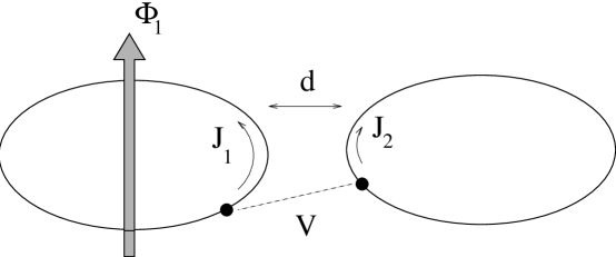
FIG. 1.: Schematic depiction of the non–dissipative drag setup. A persisent current $J_{1}$ is induced in ring 1 by a Bohm–Aharonov flux. The Coulomb interaction $V$ couples the charge fluctuations and generates a current in the second ring

The question of the effect of disorder on persistent currents remains controversial. Since our project involves calculating the effect of disorder on an induced persistent current, we expect our results to shed some light on this issue. For an isolated pure ring the persistent current is $J_{0}=ev_{F}/L$ with $L$ the perimeter of the ring and $v_{F}$ the Fermi velocity. The most immediate effect of disorder is to introduce a mean free path $\ell$. One expects disorder to decrease the persistent current, and qualitative arguments indicate that it is decreased by a factor $\ell/L$: $J_{0}\rightarrow ev_{F}/L(\ell/L)$. Our results indicate on firmer theoretical grounds that a similar argument can be used for the drag persistent current.

In this paper we outline our detailed studies of the effect of disorder on non-dissipative drag using both analytic and numerical methods.

II General remarks on the non–dissipative Drag

The zero drag current can be finite only if quantum coherence, or entanglement, between the wave functions of the two systems is established. In this situation, the meaningful description of the dynamics of the combined system involves a single wave function, which distinghuishes from ordinary dissipative drag, a case in which one has scattering between two incoherently coupled systems. Figure (1) is a schematic illustration of this coherent coupling mechanism.

FIG. 2.: Schematic depiction of the non–dissipative drag mechanism. A Bohm–Aharonov flux $\Phi$ applied in ring 1 displaces the $k$ values of the free one–particle states by $\phi/L$, with $\phi 2\pi\Phi/\phi_{0}$, $\phi_{0}$ being the flux quantum. The unperturbed energy dispersions are therefore asymmetric in ring 1 and symmetric in ring 2. When the interaction is turned on, it creates virtual excitations of momentum $-q$ in ring 1 and momentum $q$ in ring 2 (shown by the dashed arrows). The amplitude of this excitation is $V(q)/(\Delta_{1}+\Delta_{2})$. These excitations are not cancelled by those of reversed momentum (shown by the continuous arrows), the amplitude of which is $V(q)/(\Delta_{1}+\Delta_{3})$ because of the asymmetry in the spectrum of 1. As a result there is a persistent current in ring 2 proportional to $|V(q)|^{2}\phi/L$ from the terms indicated in this figure.

We consider first two one-dimensional systems. Assume that, in the absence of the Coulomb coupling, system $1$ carries a finite equilibrium current, which could in principle be established by an Aharonov-Bohm flux threading system $1$ only. If system $2$ is a one dimensional wire of perimeter $2\pi L$, the mesoscopic nature of the zero drag current can be proven by the following analysis.

Let $\Psi_{0}$ be the ground state of the combined system. This wave function involves the coordinates of both systems. Let us consider system $2$ as a closed ring geometry, and designate the coordinates of the particles in this subsystem as angular variables $\theta_{i}$, with $i=1,\cdots,N_{2}$, and $N_{2}$ being the number of particles at system 2. The kinetic component of the Hamiltonian of system $2$ can then be written as

$$H_{K}^{(2)}=-{\hbar^{2}\over 2mL^{2}}\sum_{i=1}^{N_{2}}{\partial^{2}\over\partial\theta_{i}^{2}}\;.$$ (2)

Consider the modified wave function $\Psi^{\prime}$ constructed by applying a “boost”, or gauge transformation, on the coordinates of system $2$:

$$\Psi^{\prime}=U(\alpha)\Psi_{0}\equiv\exp(i\alpha\sum_{i=1}^{N_{2}}\theta_{i})\Psi_{0},$$ (3)

with $\alpha$ a parameter. By the variational theorem $E^{\prime}=\langle\Psi^{\prime}|H|\Psi^{\prime}\rangle\geq E_{0}$, with $H$ the Hamiltonian of the combined system, and $E_{0}$ the total energy. On the other hand, explicit evaluation of $E^{\prime}$ gives

$$E^{\prime}=E_{0}+{\hbar^{2}\over 2mL^{2}}N_{2}\alpha^{2}-{h\over e}\langle\Psi_{0}|\hat{J}_{\rm Tot}^{(2)}|\Psi_{0}\rangle\,,$$ (4)

with the current operator for system $2$ given by

$$\hat{J}_{\rm Tot}^{(2)}={e\over 2\pi mL^{2}}\sum_{i=1}^{N_{2}}i\hbar{\partial\over\partial\theta_{i}}\,.$$ (5)

Due to the variational nature of the bound, the dragged current has to obey the inequality:

$$J_{\rm drag}\equiv\langle\Psi_{0}|\hat{J}_{\rm Tot}^{(2)}|\Psi_{0}\rangle\leq\alpha^{2}{e\hbar\rho\over 2\pi mL}\,,$$ (6)

with $\rho$ the particle density. Equation (6) emphasizes the mesoscopic nature of the dragged current: in the limit of $L\rightarrow\infty$, $J_{\rm drag}\rightarrow 0$ with the same length dependence as the persistent current in mesoscopic rings, the value of which is $ev_{F}/L$ in the ballistic regime. Note that the bound is valid for strictly one-dimensional systems.

Having established a bound, one needs to show that there is indeed a finite dragged current, and provide a quantitative estimate. We first present such a calculation treating the Coulomb interaction between the systems in second order perturbation theory. Consider two identical one-dimensional wires. Wire $1$ is threaded by a Aharonov-Bohm flux $\phi_{1}$ (in units of the flux quantum). In order to evaluate the induced current $J_{2}$, we impose also a flux $\phi_{2}$ in system $2$, and compute

$$J_{2}=-{e\ \over\hbar}\left.{\partial E_{0}\over\partial\phi_{2}}\right|_{\phi_{2}=0}\;.$$ (7)

We neglect the Coulomb interaction within each wire, and consider the ballistic regime (no impurities in either system). In the absence of coupling, and for both fluxes $\phi_{i}<\pi/2$, the ground state consists of two Fermi systems with one particle energies $E^{(0)}_{i}={\hbar^{2}\over 2mL^{2}}(n_{i}-\phi_{i})^{2}$, and occupied levels for $n_{i}<n_{F}$ ($i=1,2$, and $n_{F}=N/2$, $N$ being the particle number at each ring). Let $V(q)$ be the Fourier transform of the Coulomb coupling, which for wires separated a distance $d$ has the form $V(q)=(2e^{2}/L)K_{0}(qd)$, $K_{0}(x)$ being the zero-order Bessel function of imaginary argument. The second order correction to the energy is then given by:

$$\Delta E_{2}=-{mL^{2}\over\hbar^{2}}\sum_{Q,n_{1},n_{2}}{V^{2}({Q\over L})\over Q}{f_{n_{1}}(1-f_{n_{1}+Q})f_{n_{2}}(1-f_{n_{2}-Q})\over(Q+n_{1}+\phi_{1}-n_{2}-\phi_{2})}\;,$$ (8)

with $Q,n_{1},n_{2}$ integers, and $f_{m}$ Fermi functions: $f_{m}=1$ if $|m|<n_{F}$, and zero otherwise. The above sum is now evaluated transforming the sum into integrals over the continuum variables $q=Q/L$, $k_{i}=n_{i}/L$. Evaluating the integrals, and computing the derivative with respect to $\phi_{2}$, we obtain

$$J_{2}=-{me^{5}\over\hbar^{3}}{1\over 2\pi^{3}}{I(k_{F}d)\over k_{F}L}\phi_{1}\;,$$ (9)

with $I(k_{F}d)=\int_{0}^{\infty}dq{qK_{0}^{2}(qd)\over 4k_{F}^{2}-q^{2}}$. In the limit of large $k_{F}d$, which corresponds to the interparticle distance being much smaller than the distance between the systems, we obtain

$$J_{2}\simeq J_{0}{1\over(k_{F}a_{0})^{2}}{1\over(k_{F}d)^{2}}\;,$$ (10)

with $J_{0}=-ev_{F}\phi_{1}/L$ being the persistent current carried by the otherwise uncoupled system $1$, and $a_{0}$ the Bohr radius. We have proven that there is an induced persistent current due to the Coulomb interaction. We now ask ourselves about the induced effect if system $2$ is made open, so that no current can circulate. In the transport situation, a voltage will be induced. Here, we show that there is no voltage induced. We start with a setup that, in the absence of the flux in system $1$, is “parity even”. By this we mean that the charge distribution in wire $2$ is symmetric around the center of the wire. We want to know if this symmetry is broken by applying the flux in system $1$, an operation that breaks the time reversal symmetry. Let us call $P$ and $T$ the parity and time reversal operators that interchange the ends of the wire. We want for example the induced dipole moment in wire $2$, $x_{2}=\langle\Psi_{0}|\hat{x}_{2}|\Psi_{0}\rangle$. The operator $PT\hat{x}_{2}(PT)^{-1}=-\hat{x}_{2}$, while the wave function is invariant under $PT$, which implies $x_{2}=0$, hence there is no induced voltage.

III Disorder and the non–dissipative Drag

In this section we outline our results on the effect of disorder in the non–dissipative drag. In calculating the effects of disorder we use the two ring geometry considered by Rojo and Mahan, see Figure (1), and calculate the second order Coulomb interaction between the conduction electrons in the two rings. The Coulomb potential is

$\displaystyle V\equiv\sum_{k}V_{k}\rho_{k,1}\rho_{-k,2}=\int dx\int dx^{\prime}\rho_{1}(x)\rho_{2}(x^{\prime})V(x-x^{\prime}),$

With $\rho_{i}$ the charge density at ring $i$. The second order correction to the ground state energy due to the Coulomb interaction is

$$\Delta E=\sum_{n,n^{\prime}}\sum_{m,m^{\prime}}\frac{\arrowvert\sum_{k}V_{k}(\int\psi_{n}e^{i\pi kx/L}\psi_{n^{\prime}}^{\ast}dx)(\int\psi_{m}e^{i\pi kx^{\prime}/L}\psi_{m^{\prime}}^{\ast}dx^{\prime})f_{n^{\prime}}(1-f_{n})f_{m^{\prime}}(1-f_{m})\arrowvert^{2}}{E_{n}-E_{n^{\prime}}+E_{m}-E_{m^{\prime}}},$$ (11)

where $\psi_{n}$ is an eigenstate in the presence of disorder. From this expression for the energy shift we can calculate the drag current from Equation (1).

A Analytics

In this section we estimate the effect of disorder on the non-dissipative drag current for the case in which disorder is present only in the ring on which the Bohm–Aharonov flux is applied. The driven ring (ring 2), on which the drag current circulates, will be taken as disorder-free. Momentum remains a good quantum number in ring 2 making the calculation more tractable. The first order correction to the wave function is given by

$$|\Psi_{1}\rangle=\sum_{q}V(q)\sum_{k}\sum_{\bar{\nu}}{c^{\dagger}_{k+q}c_{k}|F_{2}\rangle|{\bar{\nu}}\rangle\langle{\bar{\nu}}|\rho_{q}|\psi_{0}^{(1)}\rangle\over E_{k+q}-E_{k}+E_{\bar{\nu}}-E_{0,1}},$$ (12)

where $E_{k}$ are the one-particle energies for the states of ring 2, and $|{\bar{\nu}}\rangle$ is a many-body state of ring 1 with energy $E_{\bar{\nu}}$. The ground state of ring 1 is $|\psi_{0}^{(1)}\rangle$, and its energy is $E_{0,1}$. Now, since we are neglecting interactions within each ring, the resulting equilibrium current in ring 2 is given by

$$J_{2}={e\over L}\sum_{q}{\hbar q\over m}|V(q)|^{2}\sum_{k}\sum_{\mu,\nu}{f_{k}(1-f_{k+q})f_{\mu}(1-f_{\nu})|\langle\mu|e^{iqx}|\nu\rangle|^{2}\over(E_{k+q}-E_{k}+E_{\nu}-E_{\mu})^{2}},$$ (13)

where now $|\nu\rangle$ refers to the exact one-particle states with energies $E_{\nu}$ corresponding to the disordered Hamiltoninan in ring 1. We can rewrite the above espression in terms of the spectral function $S(q,\omega)$ defined as

$$S(q,\omega)=\sum_{\mu,\nu}f_{\mu}(1-f_{\nu})|\langle\mu|e^{iqx}|\nu\rangle|^{2}\delta\left(\omega-(E_{\nu}-E_{\mu})/\hbar\right).$$ (14)

We will consider the function $S(q,\omega)$ in the approximation in which the matrix element $|\langle\mu|\rho_{q}|\nu\rangle|$ is given by the diffusive lorentzian[14]:

$$|\langle\mu|e^{iqx}|\nu\rangle|^{2}={1\over\pi\hbar N(0)}{Dq^{2}\over(Dq^{2})^{2}+(E_{\mu}-E_{\nu})^{2}/\hbar^{2}},$$ (15)

where $D$ is the difussion constant and $N(0)$ is the density of states of the system. In this approximation we obtain that $S(q,\omega)$ is given by

$$S(q,\omega)=N(0){\omega\,Dq^{2}\over(Dq^{2})^{2}+\omega^{2}}.$$ (16)

Before replacing this expression in Equation (13) let us recall that there is a flux $\Phi$ threading ring 1 and therefore one expects $S(q,\omega)\neq S(-q,\omega)$. We follow Ambegaokar and Eckern[10] in including the effect of the flux in the diffusive motion through the replacement:

$$Dq^{2}\rightarrow D\bar{q}^{2}\equiv D\left(q-\pi{\phi\over L}\right)^{2},$$ (17)

with $\phi$ being the flux in units of the flux quantum.

The induced current will therefore be given by

$$J_{2}={e\over L}\sum_{q}{\hbar q\over m}|V(q)|^{2}\hbar D\bar{q}^{2}N(0)\sum_{k}\int d\omega{f_{k}(1-f_{k+q})\over(E_{k+q}-E_{k}+\hbar\omega)^{2}}{\omega\over(D\bar{q}^{2}+\omega^{2})}.$$ (18)

For small wavevectors ($q\ll k_{F}$) we have:

$$\sum_{k}{f_{k}(1-f_{k+q})\over(E_{k+q}-E_{k}+\hbar\omega)^{2}}={L\over 2\pi}{q\over\left({\hbar^{2}\over m}k_{F}q+\hbar\omega\right)^{2}},$$ (19)

and also, in the limit of $q\ell<1$, with $\ell$ being the mean free path:

$$\int_{0}^{\infty}d\omega{1\over\left({\hbar^{2}\over m}k_{F}q+\hbar\omega\right)^{2}}{\omega\over(D\bar{q}^{2})^{2}+\omega^{2}}\simeq{(\bar{q}\ell)\over(\hbar v_{F})^{2}q^{2}}.$$ (20)

We are interested in the lowest order in $\phi$ for the induced current, which gives

$$J_{2}={e\over 4\pi}N(0){D\ell\over mv_{F}^{2}}{\phi\over L}\sum_{q}q^{2}V(q)^{2},$$ (21)

which we can now rewrite using $D=v_{F}\ell$ as

$$J_{2}\sim\left[\left({ev_{F}\over L}\right)\left({\ell\over L}\right)\right]\left[{\ell\over d}{N(0)(e^{2}/d)^{2}C\over E_{F}}\right]\times\phi,$$ (22)

where $C$ is a constant,

$$C=\int_{0}^{\infty}dxx^{2}K_{0}(x)^{2}=.308425$$ (23)

The first term in square brackets in Equation (22) corresponds to a familiar expression for the persistent current in ring 1 in the presence of disorder. The value of terms in the second square bracket can be computed taking $N(0)=1/\Delta$, with $\Delta\sim 10K$ being the level spacing for a ring of $L\sim 1\mu m$, $E_{F}=2eV$, and a distance between rings of $d=100$Å. Note that this term contains the product of two ratios: a small one given by $E_{\rm Coul}/E_{F}$, with $E_{\rm Coul}=e^{2}/d$, and a large one given by $E_{\rm Coul}/\Delta$. This gives a number of order one, a result that probably overestimates the drag current, but serves as an indication that the effects of disorder are not extreme. The second square bracket also contains an additional ratio, the mean free path to the distance between rings. This additional factor shows that the effects of disorder are stronger in the drag current from that in the driving ring. In order to test this results we performed numerical simulations, which we present in the following sections.

B Numerical simulations

1 Perturbative treatment of the Coulomb interation

In evaluating the drag current computationally we consider a discrete ring with $N$ lattice sites and $P<N$ electrons. We model disorder by placing a random disorder potential at each lattice site. The hamiltonian for an electron hopping between lattice sites in this ring is given by

$\displaystyle H=t(\sum_{i=1}^{N}C^{\dagger}_{i}C_{i+1}e^{i\phi}+\sum_{i}C^{\dagger}_{i-1}C_{i}e^{-i\phi})+\sum_{n=1}^{N}W_{n}C_{n}^{\dagger}C_{n},$

where $\phi$ is the magnetic flux through the ring, $C^{\dagger}_{i}$ is the electron creation operator at site $i$ and $w_{n}$ is the disorder potential at site $n$. For $N$ lattice sites, this gives an $N\times N$ hopping matrix.

In computing the energy shift for the two ring system we work with the x space representation of Equation (11),

$$\Delta E=\sum_{n,n^{\prime}=1}^{N}\sum_{m,m^{\prime}=1}^{N}\frac{|\sum_{x}\sum_{x^{\prime}}V(x-x^{\prime})<x|n><n^{\prime}|x><x^{\prime}|m><m^{\prime}|x^{\prime}>f_{n^{\prime}}(1-f_{n})f_{m^{\prime}}(1-f_{m})|^{2}}{E_{n}-E_{n^{\prime}}+E_{m}-E_{m^{\prime}}}.$$ (24)

Here $x$ and $x^{\prime}$ denote discrete positions of the lattice sites in rings one and two respectively and the $|n>$’s and $E_{n}$’s are the eigenvectors and eigenvalues obtained numerically from the hopping matrix. We obtain disorder averaging by evaluating $\Delta E$ with different realizations of the random disorder potentials, $W_{n}$, at values between $-W$ and $W$ where $W$ is the disorder amplitude. The result of the computer simulations are shown in figure (3) for a system of 10 lattice sites and 7 particles. The ratio of the drag current to its zero disorder value $J_{d}/J_{d}(0)$ is plotted both for a system in which disorder is present in ring 2 only and for a system of two disordered rings. The ratio $J_{o}/J_{o}(0)$ is also plotted. For small disorder amplitude, $J_{d}\propto W^{2}$.

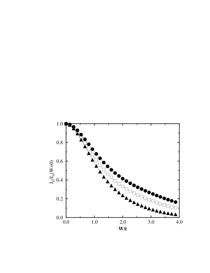
FIG. 3.: Plot of Drag Current vs. Disorder Amplitude for a system of 10 lattice sites and 7 particles with disorder averaging. We show three curves: $J_{d}/J_{d}(0)$ for one disordered ring (square symbols), $J_{d}/J_{d}(0)$ for both rings with disorder (triangles) and $J_{o}/J_{o}(0)$ (circles).

2 Non-perturbative treatment for very small rings by Lanczos method

In this section we present some exact results for small clusters. We use the Lanczos method to diagonalize the problem, and obtain results that are non–perturbative in the interaction. As a first illustration, Figure (4) shows the persistent and drag currents both with and without disorder. The drag current follows the persistent current of ring 1 in its periodicity of one flux quantum as a function of the applied flux through ring 1.

FIG. 4.: Exact results for the persistent current and the drag current as a function of flux for two rings of six sites, each of them with two particles. We show curves for zero disorder as well as finite disorder.

Figure (5) shows the drag current for two systems of different sizes. Note that the dependence with disorder is stronger for the larger system as expected from the factors of $\ell/L$ that appear in the analytical expressions in section III A.

FIG. 5.: Exact results for the drag current as a function of disorder amplitude $W$ in units of the hopping matrix element for two rings interacting via a delta function potential of amplitude $0.5t$. The flux in ring 1 is $\Phi_{1}=0.2\phi_{0}$

In conclusion we have established that the drag current remains finite for finite disorder. We have shown by numerical simulations of finite clusters and by analytical considerations that the effect of disorder on the drag current is more pronounced than the effect of disorder on the persistent current in a single ring.

REFERENCES

- [1] T. J. Gramila, J. P. Eisenstein, A. H. MacDonald, L. N. Pfeiffer and K. W. West, Phys. Rev. Lett. 66, 1216 (1991).
- [2] P. M. Solomon, P.J. Price, D. J. Franck and D. C. La Tulipe, Phys. Rev. Lett. 63 2508 (1989).
- [3] T. J. Gramila, J. P. Eisenstein, A. H. MacDonald, L. N. Pfeiffer and K. W. West, Phys. Rev. B 47; Physica B 197, 442 (1994).
- [4] M. B. Pogrebinskiĭ, Fiz. Tekh, Poluprovodn. 11, 637 (1977) [Sov. Phys. Semicond. 11, 372 (1977)]
- [5] P.J. Price, Physica 117/118 BC, 750 (19 83).
- [6] Antti-Pekka Jauho.Phys. Rev. B 47, 4420 (1993)
- [7] L.Zheng and A.H.MacDonald Phys. Rev. B 48, 8203 (1993)
- [8] H.C.Tso and P.Vasilopoulos Phys. Rev. Lett. 68, 2516 (1992)
- [9] M.Buttiker, Y.Imry, and R.Landauer Phys. Lett. 96A 365 (1983)
- [10] V. Ambegaokar and U. Eckern Phys. Rev. Lett 65 381 (1990)
- [11] A. Schmid Phys. Rev. Lett 66 80 (1991).
- [12] A.G.Rojo and G.D.Mahan Phys. Rev. Lett. 68 2074 (1992).
- [13] A.G.Rojo “Electron drag effects in coupled electron systems”, review article to be published in Journal of Physics C.
- [14] Y.Imry Introduction to Mesosc. phys. Oxford University Press. 201 (1997)
- [15] R. E. Prange and S. M. Girvin, The Quantum Hall Effect, Springer Verlag, New York (1997).
- [16] M. P. Lilly, J. P. Eisenstein, L. N. Pfeiffer and K. W. West, Phys. Rev. Lett. 80 1714 (1998).
- [17] P. Mohanty, E. M. Q. Jariwala and R. A. Webb, Phys. Rev. Lett. 78, 3366 (1997).
- [18] M. Vavilov and V. Ambegaokar, preprint cond-mat/9709241.
- [19] For recent monograhs in mesoscopic systems see: Y.Imry, Introduction to mesoscopic systems (Oxford University Press, 1997); S. Datta, Electronic Transport in Mesoscopic Systems (Cambridge University Press, 1995).
- [20] M. Büttiker, Y. Imry and and R. Landauer, Phys. Lett. 96A, 365 (1983).